Abstract
Recent denoising methods based on diffusion models typically formulate the task as a conditional generation process initialized from a standard Gaussian distribution. However, such stochastic initialization often leads to redundant sampling steps and unstable results due to the neglect of structured noise characteristics. To address these limitations, we propose a novel framework that directly bridges the probabilistic distributions of noisy and clean images while jointly modeling structured noise. We introduce Dual-diffusion Brownian Bridge Coupled Sampling (DBBCS) the first framework to incorporate Brownian bridge diffusion into image denoising. DBBCS synchronously models the distributions of clean images and structural noise via two coupled diffusion processes. Unlike conventional diffusion models, our method starts sampling directly from noisy observations and jointly optimizes image reconstruction and noise estimation through a coupled posterior sampling scheme. This allows for dynamic refinement of intermediate states by adaptively updating the sampling gradients using residual feedback from both image and noise paths. Specifically, DBBCS employs two parallel Brownian bridge models to learn the distributions of clean images and noise. During inference, their respective residual processes regulate each other to progressively enhance both denoising and noise estimation. A consistency constraint is enforced among the estimated noise, the reconstructed image, and the original noisy input to ensure stable and physically coherent results. Extensive experiments on standard benchmarks demonstrate that DBBCS achieves superior performance in both visual fidelity and quantitative metrics, offering a robust and efficient solution to image denoising.
1. Introduction
Image structural noise denoising is a specialized yet crucial task in image restoration that aims to remove structured noise artifacts and recover a clean representation of the underlying scene. Unlike random Gaussian noise, structural noise often exhibits spatial regularities and follows specific patterns or distributions. Typical examples include text overlays, shadows, watermarks, and logos, all of which are elements that occlude key image content and interfere with downstream visual tasks. The presence of structural noise significantly complicates image understanding and analysis. Because the same noisy image may correspond to multiple clean-noise combinations, the problem is inherently ill-posed [1,2]. Furthermore, structured noise often overlaps with semantically meaningful regions, making its removal more challenging than traditional noise types. Effective structural noise removal enhances the preservation of semantic information and improves the robustness of downstream tasks such as object detection, image segmentation, and feature matching. As such, developing principled and robust approaches to structural noise denoising is not only necessary but also of growing importance in various computer vision applications.
Before the emergence of deep learning, traditional denoising methods commonly relied on explicit regularization to constrain the solution space. These methods incorporated prior knowledge of clean images through various models, including non-local self-similarity models [3,4], sparse representations [5,6], gradient-based models [7], and Markov random fields [8]. However, these approaches generally require strong assumptions and tend to lack robustness. Recently, diffusion models have shown great performance in image denoising and attracted much attention. These models use score matching to approximate data gradients in noisy conditions and reverse the diffusion process to restore clean images. Thanks to their strong generative power, they have been applied in fields such as text-to-image generation and medical imaging. In image denoising, Zhang et al. [9] proposed a method starting from a normal distribution sample guided by the noisy image, while Xie et al. [10] introduced a strategy starting directly from the noisy image without Gaussian initialization.
Despite the growing body of research on image denoising using diffusion models, the field faces three critical challenges when addressing structured noise. First, existing score-based diffusion methods are primarily designed for unstructured noise and rely on simplistic noise assumptions (e.g., Gaussian or Poisson distributions), leading to underperformance on real-world images contaminated by spatially correlated, semantically meaningful, or complex-patterned structured noise. Second, the noise perturbation schemes in current diffusion models—typically adding isotropic noise during training and initializing sampling from a standard Gaussian distribution during inference—fail to capture intricate dependencies in structured degradations, resulting in redundant steps and increased uncertainty in denoising trajectories. Third, existing approaches rarely explicitly model the distribution of structured noise itself, lacking targeted guidance for the denoising process and hindering optimal reconstruction performance.
To address the limitations of existing diffusion models in structural noise denoising, we propose a new framework named Dual-diffusion Brownian Bridge modeling with Coupled Sampling (DBBCS). First, by modeling clean images and noisy images as two endpoints of Brownian bridge processes, DBBCS directly learns the bidirectional mapping between noisy observations and clean images, eliminating Gaussian initialization bias. Second, DBBCS designs parallel conditional Brownian bridge models for joint modeling of clean images and structured noise, providing abundant guidance via synchronous domain feature learning in training and coupled sampling with reciprocal constraint in inference. Third, DBBCS adopts a gradient refinement strategy using residual feedback from image and noise paths to dynamically update sampling gradients, achieving adaptive refinement of intermediate states and lower MSE through dual-path joint adjustment. This reciprocal constraint drives collaborative optimization, ensuring robust and accurate reconstruction of the clean image.
Our main contributions are summarized as follows:
- We propose a novel structured noise denoising framework based on the Diffusion Brownian Bridge Model (DBBM), marking the first application of the DBBM to structured image denoising tasks.
- We jointly model clean images and structured noise using two conditional Brownian bridge diffusion processes, formulating the denoising task as two mutually coupled posterior sampling procedures.
- We introduce a gradient refinement strategy wherein residuals from the image and noise models are used to dynamically update each other during sampling, leading to an optimized denoising trajectory.
- Extensive experiments on diverse datasets with various types of structured noise demonstrate that our model achieves robust and superior denoising performance compared to state-of-the-art methods.
2. Related Works
Image Denoising
Image denoising stands as a foundational task in image restoration, focused on retrieving a noise-free image from its corrupted counterpart [11,12]. Conventionally, image denoising is framed as an inverse problem that seeks the most plausible clean image [13]. Early denoising approaches relied on explicit regularization to narrow the solution space, integrating prior knowledge of noise-free images through techniques such as non-local self-similarity models [14], sparse representations [15], gradient-based methods [16], and Markov random field models [17]. However, these traditional methods often suffer from over-reliance on strong assumptions, limiting their robustness in real-world scenarios. With the advancement of neural networks, deep learning-driven denoising methods have emerged as state-of-the-art solutions, spanning convolutional networks [18], generative adversarial frameworks [19], and diffusion models [20]. The shift toward neural networks gained momentum in 2012, when Burger et al. [21] demonstrated that a well-trained neural network could outperform the renowned BM3D method [22] on a large dataset of paired noisy and clean images. Residual learning [23] subsequently became a staple in denoising research. Mao et al. described an early attempt at image denoising using residual connections in REDNet [24], utilizing long skip connections between corresponding layers in a mirrored encoder–decoder architecture. A number of denoising methods use long skip connections in their design to learn the residuals between noisy and clean images. Zhang et al. [25] proposed a residual dense network, aiming to fully exploit hierarchical features with dense connections in global memory blocks, which themselves are formed by a series of densely connected convolutions. Recently, Liu et al. [26] introduced a dual-residual building block to enhance the interaction between paired operations, such as downsampling and upsampling within the network. In recent years, the effectiveness of attention mechanisms has been vigorously explored and effectively applied to image denoising tasks. Anwar et al. [27] presented one of the pioneering works that benefit from channel attention mechanisms. Subsequently, Cheng et al. [28] proposed a novel subspace attention module that projects noisy images into a learned clean subspace, allowing the reconstructed images to retain most of the original content while removing noise. Tian et al. [29] proposed a cross-transformer denoising CNN (CTNet) with a Serial Block (SB), Parallel Block (PB), and Residual Block (RB) to obtain clean images for complex scenes. Wang et al. [30] presented a robust and scalable driver drowsiness detection framework that integrates a Swin Transformer-based deep learning model with a diffusion model for image denoising.
In contrast to discriminative models, generative models typically capture the generative process of observed noisy samples by modeling ; in other words, while discriminative models focus on separating out the underlying clean image, generative models attempt to understand the fundamental principles behind the formation of noisy images. Recent years have seen generative models being explored in the realm of image denoising [31,32]. Chen et al. [31] were the first to use GANs for real noise modeling, and also established a paired training dataset for training. Recently, diffusion models [33] have demonstrated powerful image generation capabilities. Due to the stepwise denoising characteristic of the reverse process of diffusion models, many recent works have applied diffusion models to image denoising. Xiang et al. [34] proposed DDM2 for unsupervised denoising of MRI images using a diffusion denoising model. By coupling statistical self-denoising techniques with diffusion models, they allowed noisy inputs to be represented as samples generated from intermediate steps in a diffusion Markov chain, producing fine-grained denoised images without the need for ground truth labels. Xie et al. [10] approached the denoising task as a problem of estimating the posterior distribution of clean images based on noisy images. They implemented generative image denoising by applying the concept of diffusion models and redefined the diffusion process according to the noise model in the denoising task, which differs from the original diffusion process. They considered three types of noise models: Gaussian noise, gamma noise, and Poisson noise. Chung et al. [35] proposed a denoising method based on fractional reverse diffusion sampling that was trained only on coronal knee joint scans, achieving denoise even when the data were contaminated by complex noise mixtures outside the distribution of in vivo liver MRI data. They achieved fine-grained control and realistic results by refining noisy images using the fractional function to solve the reverse SDE. Liu et al. [36] introduced a novel unsupervised method for denoising low-dose CT images using a diffusion model that requires only normal-dose CT images for training. By combining a cascaded diffusion model with adaptive adjustments in maximum a posteriori estimation, their method achieved zero-shot denoising and outperformed state-of-the-art supervised and unsupervised approaches in experimental evaluations. Li et al. [37] introduced Prompt-SID, a novel prompt-learning-based framework for single-image denoising. It preserves structural details through structural encoding and diffusion-based prompt integration while addressing limitations of paired datasets and pixel loss, achieving superior performance on various datasets.
Despite advancements in diffusion-based denoising, three critical research gaps persist for structured noise scenarios. Firstly, existing diffusion methods assume that noise follows isotropic Gaussian/Poisson distributions, which fails to model the spatial correlation and pattern regularity of structured noise. This leads to incomplete noise removal or over-smoothing of image details. Secondly, conventional methods initialize sampling from a standard Gaussian distribution, which requires redundant steps to map Gaussian noise to clean images. For structured noise, this indirect trajectory introduces cumulative errors and semantic inconsistency. Thirdly, existing approaches only model clean image distributions, ignoring the distributional characteristics of the structural noise itself. This lack of dual-domain guidance makes denoising blind to noise-specific patterns, resulting in limited reconstruction accuracy.
3. Method
3.1. Problem Definition
Image denoising can be formally defined as an inverse problem. Formally, let denote a noisy image degraded by a function and let represent its corresponding clean version. The degradation process is expressed as
where denotes the parameter set linked to both the degradation function and the noise model.
Noise degradation is commonly modeled as additive, leading to the additive noise formulation
The goal of denoising is to recover the true clean image x from the observed image y. Typically, the degradation function and noise parameters are unknown; thus, we learn an approximation of the inverse function:
where and represent the denoising function and its parameters, respectively. The learned denoiser acts as a regression model mapping the noisy input y to the clean ground truth x, that is, :.
Most traditional denoising methods assume that noise follows an independent and identically distributed (i.i.d.) Gaussian distribution. However, this simplification is overly restrictive for real-world scenarios involving structured complex noise. To address this, we propose leveraging the diffusion Brownian bridge model to handle arbitrary noise distributions and signal priors . In this paper, we propose utilizing the diffusion Brownian bridge model to tackle such issues.
3.2. Preliminaries
Diffusion models [20,38] are advanced machine learning algorithms that generate high-quality data by gradually adding noise to clean samples, then learning to reverse this process. This two-phase operation, consisting of forward noise addition and reverse denoising, enables precise and detailed outputs ranging from realistic images to coherent text. In the forward diffusion phase, Gaussian noise is incrementally added to an initial clean image over T steps, producing a sequence of increasingly noisy images. The transition from to uses noise with variance (diffusion rate), a value between 0 and 1 that increases with step count. This forward process is a Markov chain [39], expressed as follows:
The forward process is deterministic, meaning that any intermediate noisy sample can be directly computed from using the marginal distribution:
where , . The reverse process is generative, starting from a fully noisy distribution and progressively removing noise to recover the original data. Key to this phase is estimating the posterior , derived via Bayes’ rule from the forward process :
Because is unknown during generation, we approximate with a Gaussian distribution that matches the posterior variance . The mean of is defined as follows:
Directly predicting from is computationally challenging. Using Equation (5) to transform the mean equation, we derive
The detailed derivation process of Equations (6) and (8) can refer to Appendix A. The model is trained by predicting the added noise, with the loss objective formulated as follows [40]:
During training, clean images are sampled from the dataset, then paired with random timesteps t and Gaussian noise to compute via Equation (5). The network learns to predict from and t, with updating performed via gradient descent. Inference starts with Gaussian noise, then iteratively applies the trained model to predict noise and compute using the posterior mean and variance until .
3.3. Diffusion Brownian Bridge Model
Classic diffusion models such as the DDPM are limited to mapping between the target distribution and Gaussian distribution, failing to establish direct bidirectional distributional links between noisy and clean images. This reliance on Gaussian initialization introduces uncertainty and redundancy into the denoising process. The Diffusion Brownian Bridge Model (DBBM) addresses this limitation by learning bidirectional transformations between any two distributions. We introduce the DBBM to construct a direct mapping between noisy observations and clean images, thereby reducing sampling redundancy and improving denoising stability. For denoising tasks involving samples X (noisy images) and Y (clean images) from distributions A and B, respectively, the DBBM models the transformation between these two domains. The diffusion Brownian bridge is a continuous-time stochastic process in which the probability distribution at each step is conditioned on both the initial and final states. Specifically, the state distribution of a Brownian bridge process evolving from at to at is provided by
where T is the predetermined total number of diffusion steps.
While Equation (10) shows that while the Brownian bridge process follows Gaussian distributions at each step, which is similar to the DDPM, the key distinction lies in distributional flexibility. Unlike the DDPM, which is constrained to Gaussian-target distribution mappings, the DBBM naturally adapts to translations between arbitrary distributions (e.g., noisy to clean images). Existing diffusion-based denoising methods attempt to mitigate the DDPM’s limitations by incorporating noisy images as conditional inputs in the reverse process, but this indirect approach still suffers from uncertainty in Gaussian-to-clean image mapping and underutilization of noise distribution information, leading to semantic inconsistencies between generated and real clean images.
3.4. Noise Addition Process
This section elaborates on the noise injection process specific to the diffusion Brownian bridge model. Unlike conventional diffusion approaches that terminate with Gaussian noise, the noise addition mechanism of the diffusion Brownian bridge targets distinct sample distributions. Suppose that two samples x and y are drawn from distributions A and B, respectively. The objective of the noise injection process is to gradually transform the initial sample x into the target sample y, with each intermediate step adhering to a Gaussian distribution. Based on this principle, the noise injection process for the diffusion Brownian bridge can be formally defined as follows:
where is the predefined variance.
It is evident that as the noise injection proceeds, intermediate noisy samples gradually transition from the initial state x to the target state y. A key observation is that because the two endpoints of the process (starting point x and terminal point y) are sampled from specific distributions, intermediate samples closer to these endpoints should incorporate less Gaussian noise. Conversely, to ensure sample diversity near the midpoint of the process, more Gaussian noise is introduced to samples in this region. We adopt the noise injection strategy for diffusion Brownian bridges outlined in [41], which defines the variance as follows:
where s is the hyperparameter that regulates the intensity of the noise, which we set to a default of . It is easy to observe that at the beginning of the noise addition process, and the variance . As the noise addition process reaches its endpoint, the variance . During the noise addition process, the variance first increases to its maximum value at the midpoint . Therefore, the sampling diversity can be adjusted through the maximum variance at the mid-step .
Based on the expression for the state at each step of the diffusion Brownian bridge process as provided by Equation (11), we can obtain the marginal distribution at each step of the noise addition process:
Based on Equations (13) and (14), the transition probabilities between consecutive steps in the noise addition process of the diffusion Brownian bridge can be determined.
According to Equation (15), at the end of the noise addition process, i.e., , we can obtain and . The forward process defines a fixed mapping from distribution A to distribution B.
3.5. Denoising Process
Unlike existing diffusion-based image denoising methods, the denoising process of diffusion Brownian bridge process starts directly from the noisy image; setting in the denoising process, it predicts based on :
where represents the mean of the sample distribution at the step, while denotes the variance of the noise added at the step. Similar to DDPM, the mean needs to be learned by a neural network with parameters based on the maximum likelihood criterion.
3.6. Objective Function
This training process is accomplished by optimizing the Evidence Lower Bound (ELBO) of the diffusion Brownian bridge process [41], which can be expressed as follows:
where represents the KL divergence. Because is equal to y in the diffusion Brownian bridge process, the first term in Equation (17) can be regarded as a constant and is ignored. By combining Equations (13) and (17) and utilizing Bayes’ theorem and the properties of Markov chains, the expression in the second term can be derived as follows:
where the mean is
where
The detailed derivation process of Equations (20)–(23) can refer to Appendix A. To train the model more effectively, we set the prediction target of the model to be a linear combination of , y, and the estimated noise [41], and the training process in Algorithm 1.
In this paper, we aim to address the task of denoising images corrupted by structural noise. To extract more information about the distribution of structural noise, we not only train the diffusion Brownian bridge model on the images themselves, but also separately on a dataset consisting purely of structural noise, where the aim is to uncover the distributional characteristics of the noise. Unlike existing image denoising methods, we utilize the extracted distributional information of the structural noise to guide the denoising process in the correct trajectory.
| Algorithm 1 Training and |
| Require: Image , Structural noise , Time step , Gaussian noise Ensure: Image model , Noise model
|
3.7. DBBCS Denoising
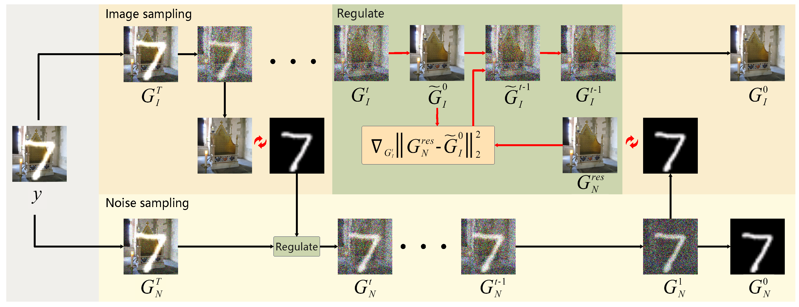
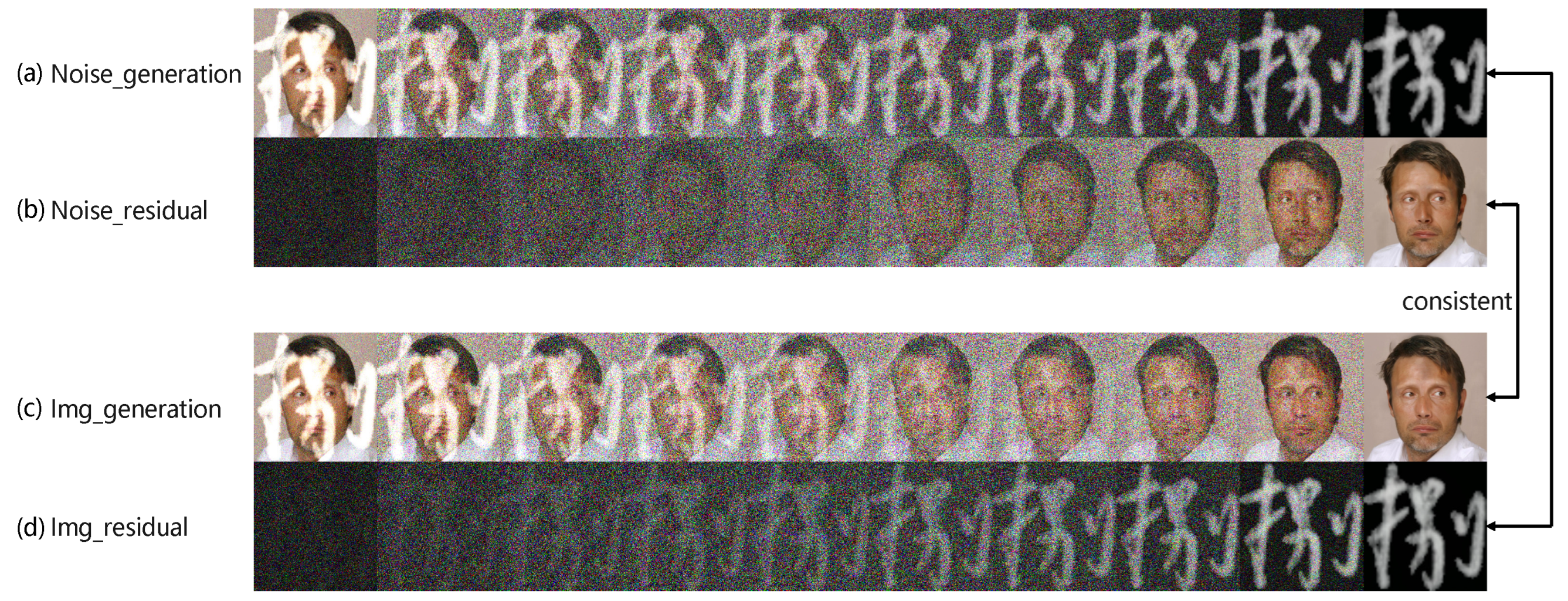
This paper is concerned with the removal of noise from images corrupted by structured noise, treating the denoising process as a posterior sampling process of the diffusion Brownian bridge. The denoising process of our method is shown in Figure 1. Specifically, we train two diffusion Brownian bridge models and on clean images and pure structured noise data, respectively, to capture the distribution characteristics of images and noise. According to the sampling feature of the diffusion Brownian bridge model, we observe that when performing posterior sampling with the trained models and , their respective residual processes correspond to each other’s generation processes, as shown in Figure 2. In other words, the residual of the posterior sampling of image model is the generation process of the structured noise. Conversely, the residual of the posterior sampling of noise model can be used to generate images.

Figure 1.
The denoising pipeline of DBBCS. The observed noisy image is directly used as the sampling starting point, and two parallel posterior sampling processes (i.e., image sampling and noise sampling) are performed simultaneously. Each step of the two posterior sampling processes is coupled with each other by using the generated intermediate samples to regulate each other. The final sampling yields the optimal image and structural noise, completing the task of robust denoising.
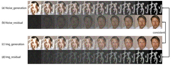
Figure 2.
(a) Posterior sampling process of structural noise (The Chinese characters in the figure are from the HWDB dataset), (b) residual process of structural noise sampling process, (c) posterior sampling process of images, and (d) residual process of image sampling process.
Based on this observation and to achieve optimal denoising results, we first conduct two posterior sampling processes simultaneously: one using model to generate clean image , and the other using model to generate structured noise . Both processes start from the noisy image y. Moreover, there is a relationship between the endpoints of these two processes. Ideally, the sum of the generated clean image and structured noise should equal the noisy image y. Leveraging this fundamental property, we propose adjusting the sampling direction in each step of the posterior sampling process using the residual from the other process. Specifically, if the two posterior sampling processes are independent, they will generate clean samples along their own sampling paths, resulting in generated samples that, when summed, may have semantically inconsistent content compared to the noisy image y. To address this, we suggest imposing a residual consistency constraint on the two posterior sampling processes to obtain optimal sampling results.
Considering that the two posterior sampling processes are iterative, samples of the image and structured noise, denoted as and , respectively, are obtained at a certain step using models and . First, the denoised image and structured noise at step t are sampled using models and :
where and are the image and structured noise samples obtained by denoising one step from and , and are the pretrained image and noise models, , , , , and are preset parameters, and is standard Gaussian noise. To couple the image and structured noise sampling processes, the image generation path is guided toward the residual of the structured noise generation result (), while the structured noise generation path is guided toward the residual of the image generation result (). Using Equations (4) and (15), we first obtain the predicted and at each generation step:
where and represent the predicted generation results at each step of the two generation processes. Consequently, their corresponding residuals and can be calculated. After obtaining the residuals from the two posterior sampling processes, we propose using a residual consistency constraint to adjust the original sampling directions of the image and structured noise. Specifically, the residual predicted by the structured noise posterior sampling serves as a guide for image posterior sampling, adjusting the movement direction of each posterior sampling step toward the residual direction of the structured noise.
After the above adjustments to each posterior sampling step, the resulting samples from the image and structured noise models are clean and maintain residual consistency.
In summary, the denoising process of our method is as follow. The observed noisy image y is directly used as the sampling starting point, and two parallel posterior sampling processes (i.e., image sampling and noise sampling) are performed simultaneously. For the t-th step of sampling, the image sample and the noise sample are estimated as clean samples and , respectively. Then, their respective residual samples are obtained by subtracting them from the original noise image y. The residual samples are input into the regulate module to adjust their respective sampling gradients, resulting in new samples and . The final sampling yields the optimal image and structural noise, completing the task of robust denoising. The denoising process in Algorithm 2.
| Algorithm 2 Structural noise denoising |
Require: T, y, ,
|
4. Experiments
4.1. Datasets
We selected multiple datasets for our experiments. Specifically, for image data (i.e., clean images), we chose the CelebA dataset and the ImageNet dataset. The CelebA dataset is a large-scale image dataset with facial attribute annotations, and is primarily used for computer vision research in face recognition and facial attribute analysis. It contains more than 10,000 different celebrities’ faces, totaling 200,000 celebrity images. ImageNet is a large visual database designed for use in image recognition, visual word, and object recognition research. It includes over 14 million labeled images distributed across approximately 20,000 categories, with an average of 1000 images per category. ImageNet’s images span a variety of objects, scenes, and animals, ranging from everyday items to very specific species. For structural noise, we also selected a variety of data for training, including the MNIST dataset, the HWDB dataset, and some synthetic noise samples. The MNIST dataset is a widely used entry-level computer vision dataset that contains grayscale images of handwritten digits. The training set contains 60,000 samples and the test set contains 10,000 samples. Each sample in the dataset is a 28 × 28 pixel grayscale image. The HWDB is a dataset of handwritten Chinese characters that is primarily used for research in Chinese character recognition and handwritten text analysis. The images in the dataset cover more than 6000 commonly used Chinese characters. Each character is written by different individuals under various conditions, including different writing styles, speeds, and stroke thicknesses. These structural noise data were used by us to add to the image data, then the denoising model was employed to remove the structural noise from the images.
4.2. Implementation Details
In order to comprehensively test the denoising effect of the DBBCS model proposed in this paper on image structural noise, we designed multiple combinations of image scenes and structural noise in the experimental section. In all experiments, we obtained noisy images using additive noise. The process of synthesizing structured noisy images involves first scaling the pixel values of clean training images (i.e., CelebA and ImageNet) and structured noise images (i.e., MNIST and HWDB) to a range of 0–1. Then, resize all images uniformly to 256 × 256. Finally, the clean training images are added to the structured noise images to obtain the structured noisy image. In addition, to test the robustness and generalization of the DBBCS model, we also tested the denoising performance of the model under conditions of out-of-distribution images and out-of-distribution noise. For our backbone network we used UNet. In the training phase, the time step of the diffusion Brownian bridge was set to 1000. The experiments were conducted on a PC with an Intel Core i5-13600k CPU@3.2. Training the network used the Adam optimizer on a PC with GHz, 24 GB RAM, and a GeForce GTX 3090 GPU. The batch size was 8 and the patch size was 256 × 256. For all benchmark datasets, the total number of iterations was set to 100,000. The learning rate of the model was 0.0002.
4.3. State-of-the-Art Methods
To validate the effectiveness of the proposed image denoising algorithm in this study, we selected eight representative contrasting algorithms for performance comparison, including four generative methods and four discriminative methods. •DDPM [40] employs forward diffusion noise-adding and reverse denoising mechanisms to reconstruct clean samples from noisy images by embedding noisy images as conditions in the reverse process. •Rectified Flow [42] enhances nonlinear feature modeling capabilities through learnable rectification steps while preserving flow field reversibility. •BBDM [41] constructs a Brownian bridge diffusion model in pixel space to achieve coherent image translation via continuous diffusion, preventing structural distortions. •GAN [19] optimizes sample authenticity iteratively through adversarial game processes between generator and discriminator networks. •SUNet [43] integrates window-based self-attention of Swin Transformer with a UNet architecture, adopting dual-sampling strategies to enhance reconstruction quality. •SwinIR [44] leverages Swin Transformer for multiscale feature fusion and residual learning to preserve image structural details. •HyLoRa [45] combines spatial self-similarity and spectral low-rank properties for joint spatial–spectral denoising in hyperspectral imaging. •CTNet [29] implements a triple-block architecture with serial blocks (deep feature extraction), parallel blocks (multilevel feature interaction), and residual blocks (final image reconstruction).
4.4. Quantitative Comparison
In order to verify the effectiveness of the image denoising algorithm proposed in this paper, the following evaluation metrics are used to quantitatively analyze the performance of the denoising algorithm. Peak Signal-to-Noise Ratio (PSNR) measures the similarity between the denoised image and the original image. The higher the PSNR value, the better the denoising effect. Structural Similarity (SSIM) evaluates the similarity between the denoised image and the original image from three aspects: brightness, contrast, and structure. The closer the SSIM value is to 1, the better the denoising effect. Mean-Square Error (MSE) measures the difference between the denoised image and the original image at each pixel point, with smaller MSE values indicating better denoising performance. Table 1 shows the comparison results of PSNR, SSIM, and MAE between our algorithm and comparison algorithms on a standard dataset, with the best results presented in bold. As shown in Table 1, our method achieved the best results on all datasets and noise types in three metrics. Specifically, our method improved the MSE metric by 0.0001 compared to the best comparison performance in four different noise modes. Improved by 0.0078, 0.0210, 0.0184, and 0.0199, respectively, compared to the worst comparison performance. Our method was also ahead of all comparison methods in terms of PSNR metrics, with numerical improvements of 2.50, 0.95, 0.20, and 0.94 compared to the best comparison method and improvements of 18.45, 14.8, 13.15, and 18.27 compared to the worst comparison method. At the same time, in terms of SSIM indicators, our method improved numerically by 0.003, 0.004, 0.009, and 0.009 compared to the best comparison method, and improved numerically by 0.212, 0.231, 0.182, and 0.230 compared to the worst comparison method. From the results, it can be seen that our method significantly improves the denoising effect of structural noise compared to the comparative algorithm. This indicates that our algorithm can effectively remove structural noise while preserving more image details.

Table 1.
The performance results of all methods in terms of MSE, PSNR, and SSIM for structural noise denoising. We represent the optimal comparison results in the bold.
4.5. Qualitative Comparison
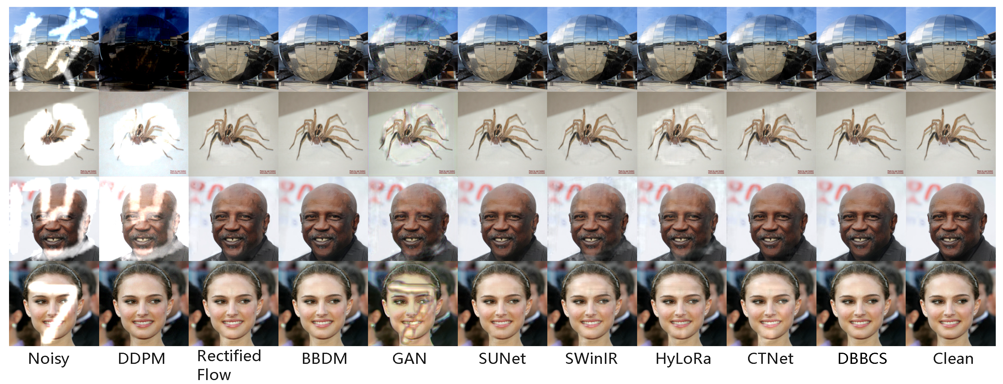
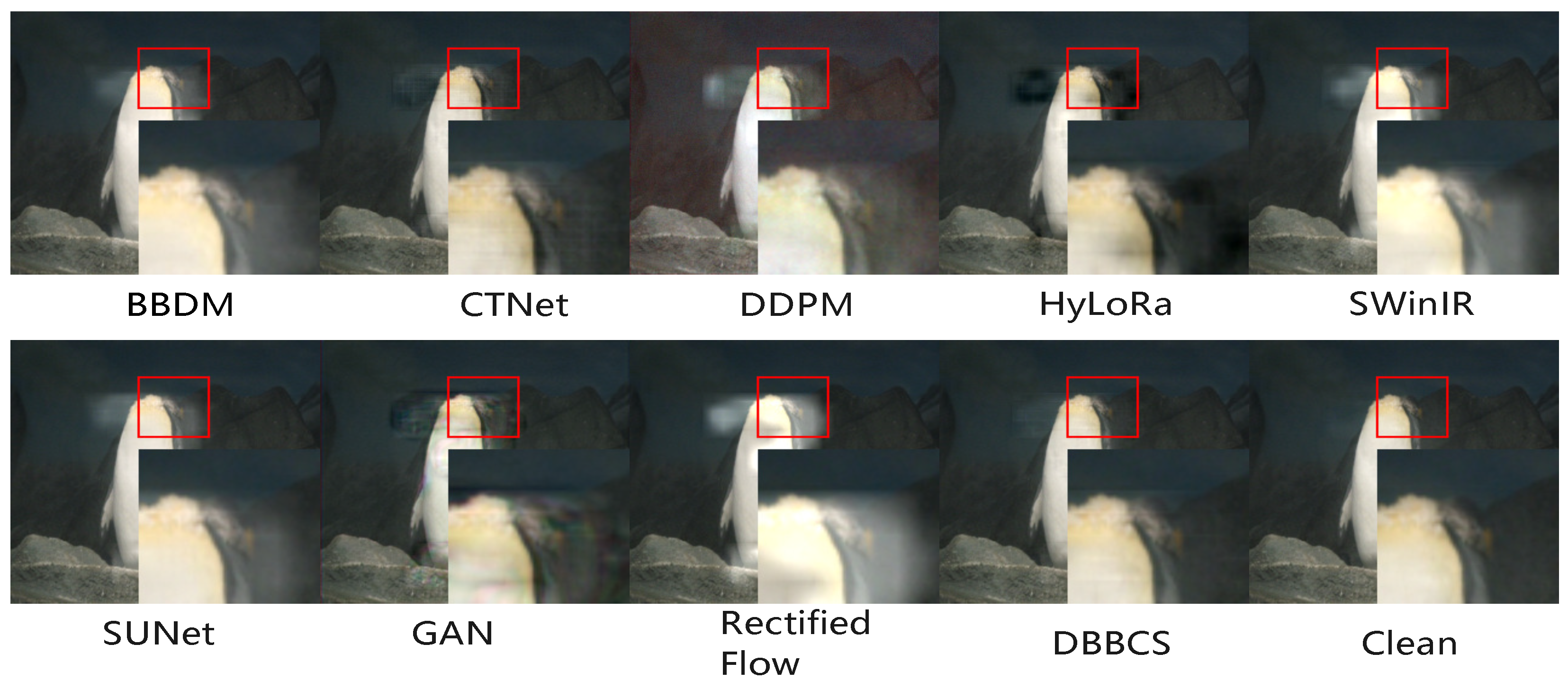
In this section, we aim to conduct a comprehensive evaluation of the performance of our proposed denoising method. The assessment is carried out through visual inspection as well as comparison with state-of-the-art existing algorithms. To perform the qualitative analysis, we meticulously examined the denoised images produced by our method, focusing on two critical aspects: preservation of image details and reduction of noise. For this analysis, we utilized a diverse test set that is a combination of two image datasets and two structural noise datasets to ensure that our evaluation covered a wide range of scenarios and challenges that a denoising method might encounter. As illustrated in Figure 3 and Figure 4, we present a visual comparison of the denoising results obtained from various algorithms when dealing with structural noise. From the figure, it is evident that our proposed method demonstrates superior performance in preserving image details. The denoised images generated by our method exhibit clear textures and well-defined edges, which are crucial elements in maintaining the overall quality and perceptual appeal of the image. Furthermore, our shows method significant effectiveness in terms of noise reduction. Relative to the comparative algorithm, our approach not only eliminates noise more efficiently but also avoids introducing obvious artificial traces. This is a crucial advantage, as the absence of artificial artifacts ensures that the denoised image appears more natural and authentic. The visual evaluation strongly demonstrates the superiority of our method in noise suppression, benefiting from the simultaneous modeling of image and structural noise distribution. Therefore, our method can simultaneously focus on the generation of the image and the removal of noise during denoising, maintaining the consistency requirements of the image and noise for the original noisy image.

Figure 3.
Comparison of visual effects of structural noise denoising by various methods. The visual fidelity of DBBCS is significantly superior to all baseline methods.
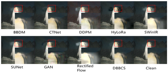
Figure 4.
Qualitative analysis of denoising results of various methods, demonstrating local denoising effects. DBBCS has the smallest artifact in a local area.
4.6. Robustness Analysis
To comprehensively assess the robustness of our proposed method and other comparative algorithms, we conducted experiments under three challenging conditions: out-of-distribution data, out-of-distribution noise, and out-of-distribution data and noise together. Such evaluation settings are designed to simulate real-world scenarios where the test data may differ significantly from the training data in terms of content or noise patterns. Specifically, all models used in the robustness tests were trained on the ImageNet+HWDB dataset to ensure a consistent training foundation. For the out-of-distribution data condition, we employed the Cebela+HWDB dataset for testing. This dataset differs from the training data in content and structural complexity, challenging the model’s ability to generalize to unseen data types. In the out-of-distribution noise condition, the ImageNet+Mnist test set was utilized. The noise characteristics in this test set diverge from those present in the training data, assessing the model’s adaptability to different noise patterns. The most demanding scenario, in which both data and noise included out-of-distribution samples, involved testing on the Cebela+Mnist test set. This condition combines both content and noise dissimilarities with the training data, providing a stringent test of the model’s generalization capabilities.
The experimental results, presented qualitatively in Figure 5 and quantitatively in Table 2, demonstrate the superior performance of our method across all three conditions. When compared to other state-of-the-art algorithms, our approach consistently achieved higher quantitative metrics and produced more visually pleasing and artifact-free denoised images.

Figure 5.
Comparison of visual effects of various methods in robust test scenarios. DBBCS generates images without obvious artifacts and has stable noise removal performance, verifying the robustness advantage of DBBCS in non-ideal scenarios.

Table 2.
The performance results of all methods in terms of MSE, PSNR, and SSIM under robust denoising scenarios. We represent the optimal comparison results in the bold.
A detailed examination of the results reveals interesting insights. As expected, in the out-of-distribution noise and out-of-distribution data and noise conditions, the denoising performance of most methods experienced some degradation, including ours. This is primarily attributed to the inconsistency between the test sets and the models’ training data. However, our method showed remarkable resilience, outperforming other algorithms in these challenging scenarios. Notably, in the out-of-distribution data condition, our method surprisingly exhibited a performance improvement. We attribute this to the diverse and complex nature of the ImageNet dataset used in training. The extensive variety of scenes and structures within ImageNet likely endowed our trained model with richer feature representations and stronger generalization abilities. In contrast, models trained on the relatively simpler Cebela dataset may lack such comprehensive understanding, leading to inferior performance when encountering out-of-distribution data samples. The robustness test results collectively confirm that our proposed method possesses strong generalization capabilities even in the presence of out-of-distribution data and noise conditions. This robustness is a crucial advantage for practical image denoising applications where the model may face diverse and unpredictable data and noise conditions.
4.7. Ablation Analysis
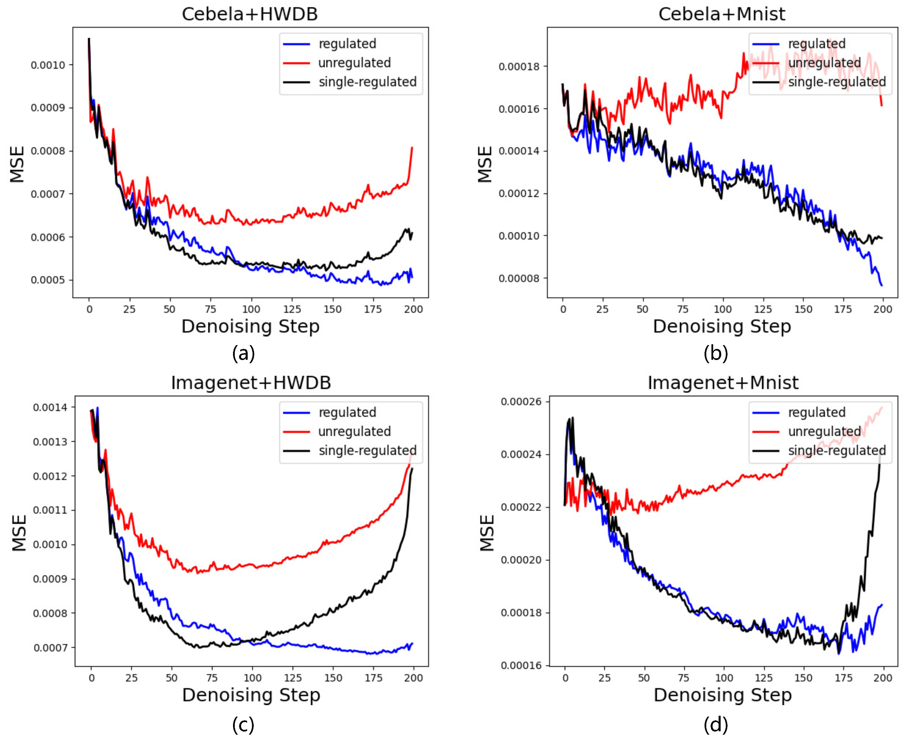
In this study, we propose a novel method that enhances the performance of structural noise denoising by modulating the posterior sampling gradient information through the residual process during sampling. To validate the effectiveness of DBBCS, we conducted a detailed ablation experiment. This experiment aimed to compare the accuracy of structural noise denoising under different regulated modes, thereby isolating the impact of our proposed modulation strategy on the overall denoising performance. Three distinct experimental scenarios were designed to evaluate the impact of different modulation strategies: an unregulated posterior sampling process, single regulation of only to the image sampling process, and simultaneous regulation of both the image and structural noise sampling processes. These three regulated modes were tested across four different structural noise scenarios to assess their robustness and effectiveness under various conditions. The Mean Squared Error (MSE) of the predicted denoised images during the posterior sampling process was calculated and served as the primary quantitative metric for comparison.
As shown in Figure 6, the unregulated posterior sampling process resulted in the highest MSE values across all structural noise scenarios, indicating poor performance in accurately reconstructing denoised images. In contrast, simultaneous regulation of both the image and structural noise sampling processes achieved the lowest MSE values, demonstrating its superiority in enhancing the accuracy of the posterior sampling process and consequently improving the denoising performance. Interestingly, single regulation of only the image sampling process led to intermediate performance, with MSE values between those of the unregulated and simultaneously regulated approaches. This suggests that while modulating the image sampling process alone can provide some improvement, the full potential of our proposed method is realized only when both the image and structural noise sampling processes are jointly regulated. These results evidence that our proposed regulated posterior sampling process is crucial for effective image denoising. By explicitly coupling the image and structural noise sampling processes through regulated sampling gradients, our method significantly improves the posterior sampling accuracy. This leads to more precise noise estimation and removal, resulting in higher-quality denoised images. The ablation study confirms that each component of our regulated strategy contributes to performance enhancement, with the most significant gains achieved when the entire coupled sampling process is regulated.
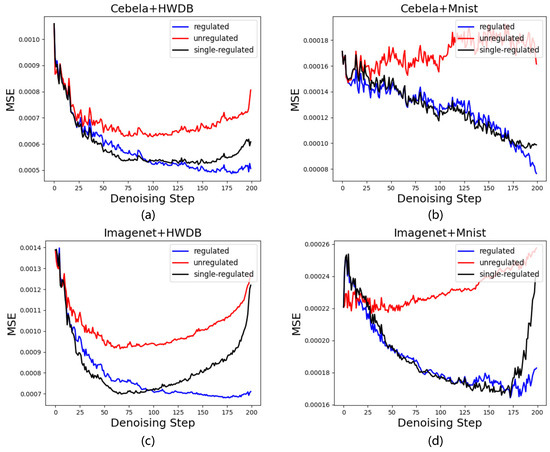
Figure 6.
(a) The impact of three different regulation strategies on denoising results on the Cebela+HWDB dataset. (b) The impact of three different regulation strategies on denoising results on the Cebela+Mnist dataset. (c) The impact of three different regulation strategies on denoising results on the ImageNet+HWDB dataset. (d) The impact of three different regulation strategies on denoising results on the ImageNet+Mnist dataset.
4.8. Impact of Regulated Strength
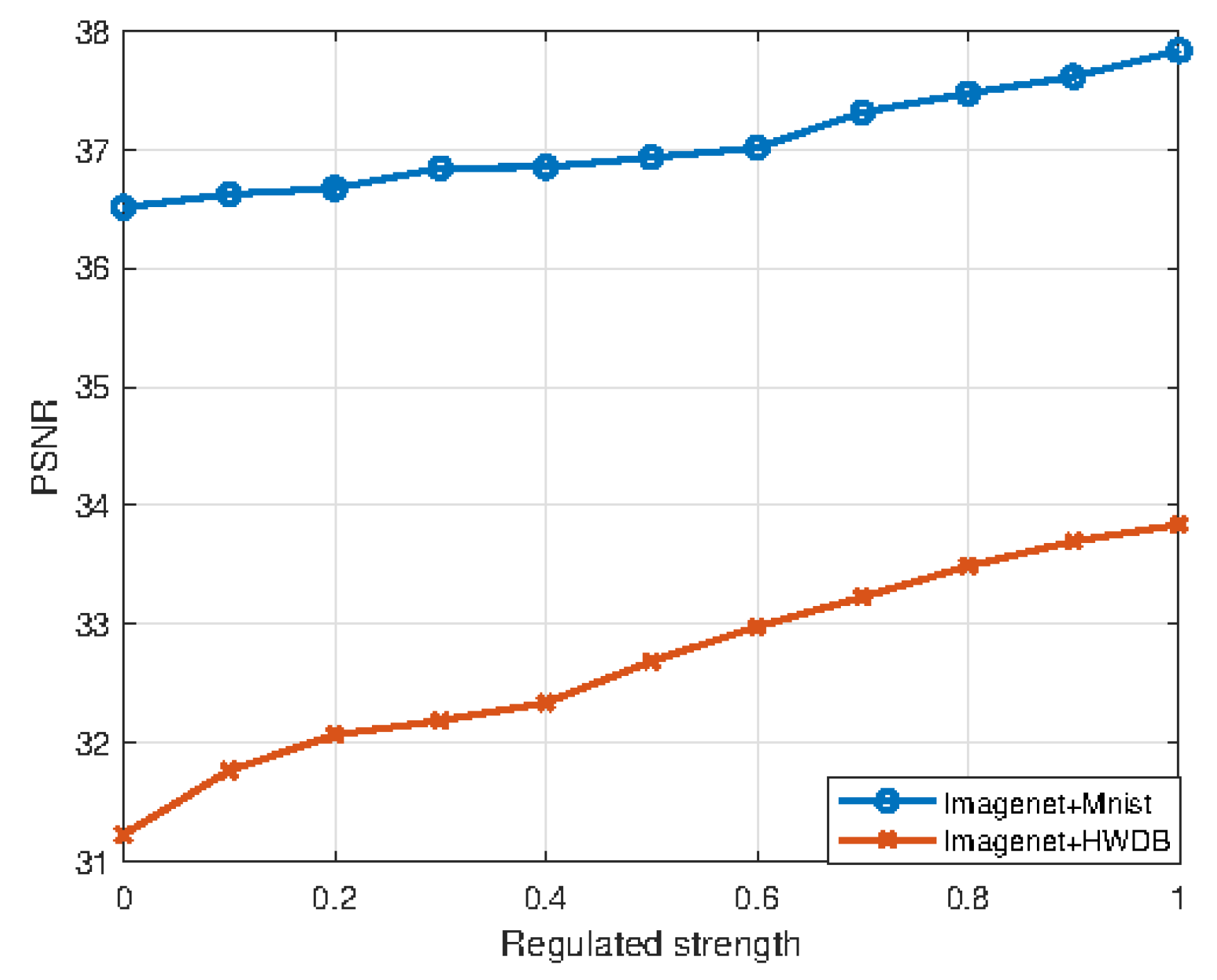
To investigate the impact of the regulated strength on denoising performance, we conducted experiments on two datasets (Imagenet+Mnist and Imagenet+HWDB) and evaluated the PSNR. In Figure 7, the x-axis represents the regulated strength (ranging from 0 to 1) and the y-axis denotes the PSNR. For the Imagenet+Mnist dataset (blue curve with circle markers), the PSNR exhibits a consistent upward trend as the regulated strength increases, rising from approximately 36.5 to nearly 38. This demonstrates that stronger regulated strength effectively enhances denoising quality for this dataset. For the Imagenet+HWDB dataset (orange curve with cross markers), the PSNR also increases with the regulated strength, climbing from around 31.2 to close to 34. However, two notable differences emerge: first, its overall PSNR values are lower than those of Imagenet+Mnist; second, the ascent rate is relatively slower in the early stage (at low regulated strengths) before accelerating in the later stage. In summary, the regulated strength is a crucial hyperparameter for denoising; increasing it improves the PSNR on both datasets, while inherent dataset differences result in variations in absolute performance levels and improvement rates.
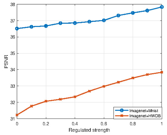
Figure 7.
The relationship between regulated strength and denoising results.
5. Conclusions
In this paper, we introduce Dual-diffusion Brownian Bridge modeling and Coupled Sampling (DBBCS), a novel framework for robust image structural noise denoising. DBBCS leverages diffusion Brownian bridge modeling to directly bridge the distributions of noisy and clean images while jointly modeling structured noise. By employing two coupled diffusion processes and a gradient refinement strategy, our method dynamically updates sampling gradients using residual feedback from both the image and noise paths, ensuring efficient and stable denoising results. Extensive experiments demonstrate that DBBCS outperforms state-of-the-art methods in both visual fidelity and quantitative metrics, offering a significant advancement in the field of image denoising. Thanks to its efficient denoising performance for structural noise, the DBBCS method also shines in practical application scenarios; for example, in document watermark removal tasks, it can effectively eliminate semi-transparent text watermarks from scanned documents while preserving printed content. It can also play an effective role in the field of medical image denoising, processing MRI images with structured artifacts such as motion artifacts. However, our work also has some limitations. The computational complexity of DBBCS is relatively high due to the dual-diffusion processes and coupled sampling mechanism, which may limit its application in real-time scenarios. Additionally, the performance of DBBCS relies heavily on the quality and diversity of the training data as well as careful tuning of hyperparameters such as the noise variance and coupling strength. Future work could focus on optimizing the computational efficiency of DBBCS, exploring more efficient sampling strategies, and developing adaptive methods for hyperparameter tuning. Furthermore, extending the DBBCS framework to other image restoration tasks such as image inpainting and super-resolution could be promising directions for future research. Overall, our work not only provides a robust solution for structural noise denoising but also opens up new avenues for the application of diffusion bridge models in low-level vision tasks. We hope that our findings will inspire further research in this area and contribute to the development of more advanced image restoration techniques.
Author Contributions
Conceptualization, L.C. and J.J.; methodology, C.Y.; software, H.X.; validation, L.C. and J.J.; formal analysis, Y.H.; investigation, L.C.; data curation, Y.H.; writing—original draft preparation, L.C.; writing—review and editing, C.Y.; visualization, H.X.; supervision, C.Y.; project administration, J.J.; funding acquisition, L.C. and J.J. All authors have read and agreed to the published version of the manuscript.
Funding
This research was funded by the Guangxi Science and Technology Program (Grant no. AB25069247, Grant no. AB25069280).
Data Availability Statement
All supporting data for this study are from publicly archived datasets. The detailed information for accessing these datasets is as follows: Cebela dataset can be obtained from http://mmlab.ie.cuhk.edu.hk/projects/CelebA.html, Mnist dataset can be obtained from http://yann.lecun.com/exdb/mnist, HWDB dataset can be obtained from http://www.nlpr.ia.ac.cn/databases/download/feature_data/HWDB1.1trn_gnt.zip, ImageNet dataset can be obtained from http://www.image-net.org, all accessed on 23 August 2025.
Conflicts of Interest
The authors declare no conflicts of interest.
Appendix A
Appendix A.1. The Derivation Process of Equations (6) and (8)
The reverse process goal of the diffusion model is to restore the noisy data to the previous step . It is very difficult to directly calculate the inverse distribution , but if the original data x are known, then the conditional distribution can be simplified by Bayes’ theorem, as follows:
Because all distributions of the forward process are Gaussian distributions, according to the properties of Gaussian distributions, the conditional posterior distribution must also consist of Gaussian distributions. We can express this as
where is the mean and is the variance.
To calculate the mean of the conditional posterior distribution, we start from Bayes’ rule and expand Equation (1) into the product of two Gaussian distributions:
According to the multiplicative property of Gaussian distributions, the product of two Gaussian distributions is still a Gaussian distribution, and its exponential part can be merged through the following combination method:
- Write the exponential parts of two Gaussian distributions:
- -
- First item:
- -
- Second item:
- Merge the items:
- Expand the square term:
- Extract the quadratic and linear terms of :
- -
- Quadratic coefficient:
- -
- Primary coefficient:
After the configuration method is completed, the mean of the new Gaussian distribution is
After algebraic simplification (using and ), the mean expression is finally obtained:
In practical applications, we are unable to obtain raw data in Equation (A7). Therefore, it is necessary to include the mean in the expression . We eliminate this utilizing the multi-step cumulative distribution of the forward process:
It can then be solved that
We substitute into the mean expression in Equation (A7):
After simplification, we obtain
Appendix A.2. The Derivation Process of Equations (20)–(23)
As shown in Equation (18),
which can be written in the form of the following Probability Density Function (PDF):
In the same way, the right part of Equation (A13) can also be represented as a PDF which contains three sub-parts.
From Equation (15), we can obtain .
The PDFs of and can also be derived based on Equations (13) and (14).
Considering that the PDFs of the left and right parts of Equation (18) must be equal, the following equation can be derived:
Then, we can obtain the equations below.
Appendix A.3. Symbols Used in This Paper
| Symbol | Description | Equation |
| y | Noisy observation image with structural noise | Equations (1) and (2) |
| x / | Clean image | Equations (1) and (2) |
| Gaussian noise | Equation (8) | |
| T | Total number of diffusion steps | Equation (10) |
| Noise intensity at the t-th forward diffusion step | Equation (4) | |
| Predefined coefficient | Equation (5) | |
| Cumulative retention coefficient up to the t-th diffusion step | Equation (5) | |
| Single-step probability distribution of forward diffusion | Equation (4) | |
| Multi-step probability distribution of forward diffusion (from to ) | Equation (5) | |
| Posterior conditional probability distribution of forward diffusion | Equation (6) | |
| Mean of the reverse diffusion distribution (learned by the neural network) | Equation (7) | |
| Clean image predicted by the neural network | Equation (7) | |
| Noise term predicted by the neural network | Equation (9) | |
| Simple loss function of the diffusion model (noise prediction MSE) | Equation (9) | |
| Endpoint state of the diffusion Brownian bridge process (set to in denoising) | Equation (10) | |
| Time weighting factor of the diffusion Brownian bridge process | Equation (11) | |
| Noise standard deviation at the t-th step of the diffusion Brownian bridge process | Equations (11) and (12) | |
| s | Scaling parameter for the noise intensity of the diffusion Brownian bridge process | Equation (12) |
| Standard deviation of the single-step transition probability of the diffusion Brownian bridge process | Equation (15) | |
| Parameterized conditional distribution of the reverse denoising process in the diffusion Brownian bridge | Equation (16) | |
| Variance of the reverse denoising process | Equation (16) | |
| ELBO | Evidence lower bound (used for optimizing the diffusion Brownian bridge model) | Equation (17) |
| KL divergence (measures the distance between two probability distributions) | Equation (17) |
Appendix A.4. The Effects of Different Experimental Settings
| Datasets | Cebela+Mnist | Imagenet+HWDB | ||||
| Metrics | MSE | PSNR | SSIM | MSE | PSNR | SSIM |
| batch = 8, patch = 256 × 256, iterations = 100,000, lr = 0.0002 | 0.0001 | 39.96 | 0.994 | 0.0005 | 33.84 | 0.975 |
| batch = 4, patch = 256 × 256, iterations = 100,000, lr = 0.0002 | 0.0001 | 39.93 | 0.991 | 0.0005 | 33.80 | 0.971 |
| batch = 8, patch = 256 × 256, iterations = 10,000, lr = 0.0002 | 0.0002 | 38.46 | 0.985 | 0.0007 | 31.27 | 0.947 |
| batch = 8, patch = 512 × 512, iterations = 100,000, lr = 0.0002 | 0.0001 | 39.90 | 0.992 | 0.0005 | 33.79 | 0.970 |
| batch = 8, patch = 256 × 256, iterations = 100,000, lr = 0.001 | 0.0001 | 39.85 | 0.986 | 0.0006 | 33.70 | 0.961 |
Appendix A.5. The Parameters and FLOPs Information of Each Model
| Model | FLOPs (G) | Parametres (M) |
| DBBCS | 398 | 12 |
| DDPM | 360 | 47 |
| Rectified Flow | 672 | 56 |
| BBDM | 288 | 15 |
| GAN | 968 | 64 |
| SUNet | 458 | 31 |
| SwinIR | 788 | 11 |
| HyLoRa | 516 | 34 |
| CTNet | 512 | 35 |
References
- Huo, Y.; Deng, Z.; Zhang, P.; Lu, Z.; Zhang, F.; Li, M.; Hou, Y.; Xi, P.; Huang, W.; Zhang, Y. DMF-SIM: Dual-Model Framework for super-resolution reconstruction and denoising in Structured Illumination Microscopy. Pattern Recognit. 2025, 169, 111865. [Google Scholar] [CrossRef]
- Liu, Z.; Zhou, W.; Guo, C.; Qiu, Q.; Xie, Z. PyramidPCD: A novel pyramid network for point cloud denoising. Pattern Recognit. 2025, 161, 111228. [Google Scholar] [CrossRef]
- Li, S.; Wang, F.; Gao, S. New non-local mean methods for MRI denoising based on global self-similarity between values. Comput. Biol. Med. 2024, 174, 108450. [Google Scholar] [CrossRef] [PubMed]
- Zhuang, L.; Fu, X.; Ng, M.K.; Bioucas-Dias, J.M. Hyperspectral image denoising based on global and nonlocal low-rank factorizations. IEEE Trans. Geosci. Remote Sens. 2021, 59, 10438–10454. [Google Scholar] [CrossRef]
- Sheng, J.; Lv, G.; Wang, Z.; Feng, Q. SRNet: Sparse representation-based network for image denoising. Digit. Signal Process. 2022, 130, 103702. [Google Scholar] [CrossRef]
- Xu, W.; Zhu, Q.; Qi, N.; Chen, D. Deep sparse representation based image restoration with denoising prior. IEEE Trans. Circuits Syst. Video Technol. 2022, 32, 6530–6542. [Google Scholar] [CrossRef]
- Li, P.; Liang, J.; Zhang, M.; Fan, W.; Yu, G. Joint image denoising with gradient direction and edge-preserving regularization. Pattern Recognit. 2022, 125, 108506. [Google Scholar] [CrossRef]
- Pleschberger, M.; Schrunner, S.; Pilz, J. An explicit solution for image restoration using Markov random fields. J. Signal Process. Syst. 2020, 92, 257–267. [Google Scholar] [CrossRef]
- Zhang, L.; Rao, A.; Agrawala, M. Adding conditional control to text-to-image diffusion models. In Proceedings of the IEEE/CVF International Conference on Computer Vision, Paris, France, 4–6 October 2023; pp. 3836–3847. [Google Scholar]
- Xie, Y.; Yuan, M.; Dong, B.; Li, Q. Diffusion model for generative image denoising. arXiv 2023, arXiv:2302.02398. [Google Scholar] [CrossRef]
- Izadi, S.; Sutton, D.; Hamarneh, G. Image denoising in the deep learning era. Artif. Intell. Rev. 2023, 56, 5929–5974. [Google Scholar] [CrossRef]
- Li, Y.; Zhang, Y.; Timofte, R.; Van Gool, L.; Tu, Z.; Du, K.; Wang, H.; Chen, H.; Li, W.; Wang, X.; et al. NTIRE 2023 challenge on image denoising: Methods and results. In Proceedings of the IEEE/CVF Conference on Computer Vision and Pattern Recognition, Vancouver, BC, Canada, 17–24 June 2023; pp. 1905–1921. [Google Scholar]
- Gkillas, A.; Ampeliotis, D.; Berberidis, K. Connections between deep equilibrium and sparse representation models with application to hyperspectral image denoising. IEEE Trans. Image Process. 2023, 32, 1513–1528. [Google Scholar] [CrossRef] [PubMed]
- Wang, J.; Guo, Y.; Ying, Y.; Liu, Y.; Peng, Q. Fast non-local algorithm for image denoising. In Proceedings of the 2006 International Conference on Image Processing, Atlanta, GA, USA, 8–11 October 2006; IEEE: New York, NY, USA, 2006; pp. 1429–1432. [Google Scholar]
- Elad, M.; Aharon, M. Image denoising via sparse and redundant representations over learned dictionaries. IEEE Trans. Image Process. 2006, 15, 3736–3745. [Google Scholar] [CrossRef] [PubMed]
- Liu, Y.; Anwar, S.; Zheng, L.; Tian, Q. Gradnet image denoising. In Proceedings of the IEEE/CVF Conference on Computer Vision and Pattern Recognition Workshops, Seattle, WA, USA, 14–19 June 2020; pp. 508–509. [Google Scholar]
- Amini, M.; Ahmad, M.O.; Swamy, M. Image denoising in wavelet domain using the vector-based hidden Markov model. In Proceedings of the 2014 IEEE 12th International New Circuits and Systems Conference (NEWCAS), Trois-Rivieres, QC, Canada, 22–25 June 2014; IEEE: New York, NY, USA, 2014; pp. 29–32. [Google Scholar]
- Zeiler, M.D.; Fergus, R. Visualizing and understanding convolutional networks. In Proceedings, Part I 13, Proceedings of the Computer Vision–ECCV 2014: 13th European Conference, Zurich, Switzerland, 6–12 September 2014; Springer: Berlin/Heidelberg, Germany, 2014; pp. 818–833. [Google Scholar]
- Goodfellow, I.; Pouget-Abadie, J.; Mirza, M.; Xu, B.; Warde-Farley, D.; Ozair, S.; Courville, A.; Bengio, Y. Generative adversarial networks. Commun. ACM 2020, 63, 139–144. [Google Scholar] [CrossRef]
- Croitoru, F.A.; Hondru, V.; Ionescu, R.T.; Shah, M. Diffusion models in vision: A survey. IEEE Trans. Pattern Anal. Mach. Intell. 2023, 45, 10850–10869. [Google Scholar] [CrossRef] [PubMed]
- Burger, H.C.; Schuler, C.J.; Harmeling, S. Image denoising: Can plain neural networks compete with BM3D? In Proceedings of the 2012 IEEE Conference on Computer Vision and Pattern Recognition, Providence, RL, USA, 16–21 June 2012; IEEE: New York, NY, USA, 2012; pp. 2392–2399. [Google Scholar]
- Dabov, K.; Foi, A.; Katkovnik, V.; Egiazarian, K. Image denoising by sparse 3-D transform-domain collaborative filtering. IEEE Trans. Image Process. 2007, 16, 2080–2095. [Google Scholar] [CrossRef] [PubMed]
- Tai, Y.; Yang, J.; Liu, X.; Xu, C. Memnet: A persistent memory network for image restoration. In Proceedings of the IEEE International Conference on Computer Vision, Venice, Italy, 22–29 October 2017; pp. 4539–4547. [Google Scholar]
- Zhang, K.; Zuo, W.; Chen, Y.; Meng, D.; Zhang, L. Beyond a gaussian denoiser: Residual learning of deep cnn for image denoising. IEEE Trans. Image Process. 2017, 26, 3142–3155. [Google Scholar] [CrossRef] [PubMed]
- Zhang, Y.; Tian, Y.; Kong, Y.; Zhong, B.; Fu, Y. Residual dense network for image super-resolution. In Proceedings of the IEEE Conference on Computer Vision and Pattern Recognition, Salt Lake City, UT, USA, 18–22 June 2018; pp. 2472–2481. [Google Scholar]
- Liu, X.; Suganuma, M.; Sun, Z.; Okatani, T. Dual residual networks leveraging the potential of paired operations for image restoration. In Proceedings of the IEEE/CVF Conference on Computer Vision and Pattern Recognition, Long Beach, CA, USA, 15–20 June 2019; pp. 7007–7016. [Google Scholar]
- Anwar, S.; Barnes, N. Real image denoising with feature attention. In Proceedings of the IEEE/CVF International Conference on Computer Vision, Seoul, Republic of Korea, 27 October–2 November 2019; pp. 3155–3164. [Google Scholar]
- Cheng, S.; Wang, Y.; Huang, H.; Liu, D.; Fan, H.; Liu, S. Nbnet: Noise basis learning for image denoising with subspace projection. In Proceedings of the IEEE/CVF Conference on Computer Vision and Pattern Recognition, Nashville, TN, USA, 19–25 June 2021; pp. 4896–4906. [Google Scholar]
- Tian, C.; Zheng, M.; Zuo, W.; Zhang, S.; Zhang, Y.; Lin, C.W. A cross Transformer for image denoising. Inf. Fusion 2024, 102, 102043. [Google Scholar] [CrossRef]
- Wang, M.; Yuan, P.; Qiu, S.; Jin, W.; Li, L.; Wang, X. Dual-Encoder UNet-Based Narrowband Uncooled Infrared Imaging Denoising Network. Sensors 2025, 25, 1476. [Google Scholar] [CrossRef] [PubMed]
- Chen, J.; Chen, J.; Chao, H.; Yang, M. Image blind denoising with generative adversarial network based noise modeling. In Proceedings of the IEEE Conference on Computer Vision and Pattern Recognition, Salt Lake City, UT, USA, 18–22 June 2018; pp. 3155–3164. [Google Scholar]
- Yue, Z.; Zhao, Q.; Zhang, L.; Meng, D. Dual adversarial network: Toward real-world noise removal and noise generation. In Proceedings, Part X 16, Proceedings of the Computer Vision–ECCV 2020: 16th European Conference, Glasgow, UK, 23–28 August 2020; Springer: Berlin/Heidelberg, Germany, 2020; pp. 41–58. [Google Scholar]
- Rombach, R.; Blattmann, A.; Lorenz, D.; Esser, P.; Ommer, B. High-resolution image synthesis with latent diffusion models. In Proceedings of the IEEE/CVF Conference on Computer Vision and Pattern Recognition, New Orleans, LA, USA, 18–24 June 2022; pp. 10684–10695. [Google Scholar]
- Xiang, T.; Yurt, M.; Syed, A.B.; Setsompop, K.; Chaudhari, A. DDM2: Self-Supervised Diffusion MRI Denoising with Generative Diffusion Models. arXiv 2023, arXiv:2302.03018. [Google Scholar]
- Chung, H.; Lee, E.S.; Ye, J.C. MR image denoising and super-resolution using regularized reverse diffusion. IEEE Trans. Med. Imaging 2022, 42, 922–934. [Google Scholar] [CrossRef] [PubMed]
- Liu, X.; Xie, Y.; Liu, C.; Cheng, J.; Diao, S.; Tan, S.; Liang, X. Diffusion probabilistic priors for zero-shot low-dose CT image denoising. Med. Phys. 2025, 52, 329–345. [Google Scholar] [CrossRef] [PubMed]
- Li, H.; Zhang, W.; Hu, X.; Jiang, T.; Chen, Z.; Wang, H. Prompt-SID: Learning Structural Representation Prompt via Latent Diffusion for Single Image Denoising. Proc. AAAI Conf. Artif. Intell. 2025, 39, 4734–4742. [Google Scholar] [CrossRef]
- Zhu, Y.; Zhang, K.; Liang, J.; Cao, J.; Wen, B.; Timofte, R.; Van Gool, L. Denoising diffusion models for plug-and-play image restoration. In Proceedings of the IEEE/CVF Conference on Computer Vision and Pattern Recognition, Vancouver, BC, Canada, 17–24 June 2023; pp. 1219–1229. [Google Scholar]
- Teng, H.; Quan, Y.; Wang, C.; Huang, J.; Ji, H. Fingerprinting Denoising Diffusion Probabilistic Models. In Proceedings of the Computer Vision and Pattern Recognition Conference, Nashville, TN, USA, 11–15 June 2025; pp. 28811–28820. [Google Scholar]
- Ho, J.; Jain, A.; Abbeel, P. Denoising diffusion probabilistic models. Adv. Neural Inf. Process. Syst. 2020, 33, 6840–6851. [Google Scholar]
- Li, B.; Xue, K.; Liu, B.; Lai, Y.K. Bbdm: Image-to-image translation with brownian bridge diffusion models. In Proceedings of the IEEE/CVF Conference on Computer Vision and Pattern Recognition, Vancouver, BC, Canada, 17–24 June 2023; pp. 1952–1961. [Google Scholar]
- Lee, S.; Lin, Z.; Fanti, G. Improving the training of rectified flows. Adv. Neural Inf. Process. Syst. 2024, 37, 63082–63109. [Google Scholar]
- Fan, C.M.; Liu, T.J.; Liu, K.H. SUNet: Swin transformer UNet for image denoising. In Proceedings of the 2022 IEEE International Symposium on Circuits and Systems (ISCAS), Austin, TX, USA, 28 May–1 June 2022; pp. 2333–2337. [Google Scholar]
- Liang, J.; Cao, J.; Sun, G.; Zhang, K.; Van Gool, L.; Timofte, R. Swinir: Image restoration using swin transformer. In Proceedings of the IEEE/CVF International Conference on Computer Vision, Montreal, BC, Canada, 11–17 October 2021; pp. 1833–1844. [Google Scholar]
- Tan, X.; Shao, M.; Qiao, Y.; Liu, T.; Cao, X. Low-Rank Prompt-Guided Transformer for Hyperspectral Image Denoising. IEEE Trans. Geosci. Remote Sens. 2024, 62, 1–15. [Google Scholar] [CrossRef]
Disclaimer/Publisher’s Note: The statements, opinions and data contained in all publications are solely those of the individual author(s) and contributor(s) and not of MDPI and/or the editor(s). MDPI and/or the editor(s) disclaim responsibility for any injury to people or property resulting from any ideas, methods, instructions or products referred to in the content. |
© 2025 by the authors. Licensee MDPI, Basel, Switzerland. This article is an open access article distributed under the terms and conditions of the Creative Commons Attribution (CC BY) license (https://creativecommons.org/licenses/by/4.0/).

