Abstract
Human motion exhibits high-dimensional and stochastic characteristics, posing significant challenges for modeling and prediction. Existing approaches typically employ coupled spatiotemporal frameworks to generate future poses. However, the intrinsic nonlinearity of joint interactions over time, compounded by high-dimensional noise, often obscures meaningful motion features. Notably, while adjacent joints demonstrate strong spatial correlations, their temporal trajectories frequently remain independent, adding further complexity to modeling efforts. To address these issues, we propose a novel framework for human motion prediction via the decoupled spatiotemporal clue (DSC), which explicitly disentangles and models spatial and temporal dependencies. Specifically, DSC comprises two core components: (i) a spatiotemporal decoupling module that dynamically identifies critical joints and their hierarchical relationships using graph attention combined with separable convolutions for efficient motion decomposition; and (ii) a pose generation module that integrates local motion denoising with global dynamics modeling through a spatiotemporal transformer that independently processes spatial and temporal correlations. Experiments on the widely used human motion datasets H3.6M and AMASS demonstrate the superiority of DSC, which achieves 13% average improvement in long-term prediction over state-of-the-art methods.
1. Introduction
Human motion prediction is a complex spatiotemporal modeling issue that has been a longstanding and challenging research topic in the field of computer vision. Due to its importance in modeling and understanding human behavior, 3D human motion prediction has applications in areas such as animation [1], motion synthesis [2], and human–computer interaction [3,4,5]. Future extensions may enable deployment in more complex environments, including autonomous systems and augmented/virtual reality.
Accurate prediction of human motion relies on the effective modeling of spatiotemporal correlations, joint interactions, and temporal dynamics. Current approaches mainly employ strategies: temporal modeling through temporal convolutional networks (TCNs) [6,7], recurrent neural networks (RNNs) [8,9,10,11], gated recurrent units (GRUs) [12,13], long short-term memory networks (LSTMs) [14], or Transformer [15,16,17]; spatial modeling via graph-based methods, like graph convolutional networks (GCNs) [18,19], with advanced variants, such as dynamic multi-scale graph neural networks (DMGNN) [20] and multi-scale residual GCN (MSR-GCN) [21]), capture multi-scale relationships. While such isolated spatial or temporal modeling reduces complexity, it inherently fails to capture the nuanced interplay of human kinematics. In reality, the high-dimensional stochasticity of human motion weakens idealized spatiotemporal correlations (as shown in Figure 1). Our analysis reveals a critical issue: while adjacent joints exhibit strong spatial coupling, their temporal trajectories evolve with surprising independence. This divergence implies that forcibly coupling spatiotemporal features, as in existing methods, risks obscuring the discriminative patterns within noise, demanding more principled architectural designs. To address the confusion caused by forced spatiotemporal feature coupling in existing models, we propose a novel prediction framework that can explicitly comprehend relationships via Decoupled Spatiotemporal Clue (DSC). DSC consists of two primary components that together enable precise future pose synthesis: a spatiotemporal decoupling module (SDM) for independent feature learning, and a pose generation module (PGM) for specialized temporal and spatial modeling.
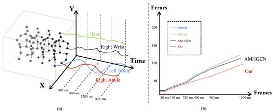
Figure 1.
Spatial correlation and temporal independence in human motion. (a) When a person is walking, there exists intrinsic spatial correlations among body joints, yet each joint exhibits independent motion trajectories over time. (b) The performance comparison of different methods on the H3.6M [22] dataset based on average results under the Mean Per Joint Position Error (MPJPE) metric. PPGMP [23]: Pose Propagation with Graph-based Motion Prediction; SiMLpe [24]: Simplified Multi-Layer Pose Estimation; and AMHGCN [25]: Adaptive Multi-Hierarchy Graph Convolutional Network.
The SDM explicitly models the independence of the joint motion trajectories within human pose representations. Utilizing a decoupled spatiotemporal encoding scheme, this module effectively captures the distinct spatiotemporal feature relationships through two complementary components: (i) a graph attention component (GAC) that dynamically learns multi-level joint dependencies, and (ii) a spatiotemporal decoupling encoding component (SDEC) for hierarchical feature extraction. The GAC overcomes limitations of conventional graph convolutional networks by replacing fixed skeletal graphs with an attention mechanism. This enables the adaptive modeling of cross-joint dependencies across semantic levels, where critical joints automatically receive higher weights based on their topological and functional significance. The SDEC employs parallel temporal and spatial processing streams. Temporal convolutions capture the motion trajectory features along the time dimension, while spatially constrained convolutions preserve the kinematic relationships between joints. Through an interpretation of channel dimensions as temporal scales, the SDEC achieves efficient multi-resolution feature extraction while strictly decoupling the temporal dynamics from structural semantics. These components generate a disentangled representation that captures both the temporal evolution and spatial configuration of human motion.
The aim of the PGM is to accurately predict future human pose sequences through independent temporal and spatial dependencies. This module consists of two parts: a temporal feature extraction (TFE), and a spatiotemporal decoupled Transformer (STDT). The TFE stage utilizes two 1D convolutions with rectified linear unit (ReLU) activations, sliding solely along the temporal axis to capture the local motion patterns between adjacent frames without incorporating spatial dimensions. This processing attenuates high-frequency noise while standardizing local features, thereby providing cleaner, higher-order inputs for subsequent deep attention mechanisms. Within the STDT, we depart from conventional Transformer architectures by designing four distinct, independently parameterized attention modules: spatial, temporal, spatiotemporal crossover, and global. Each module learns its own projection matrices, preventing spatiotemporal feature coupling during parameter updates. This explicit decoupling enables the direct visualization of attention weights, clarifying the source of learned dependencies. Critically, because the spatial module explicitly models the joint topology, the temporal module is dedicated solely to dynamic evolution. We posit that single-head attention acts as an effective “temporal smoother” for spatial features, whereas multi-head attention may introduce noisy interactions. Consequently, the STDT employs a single-head design. Following TFE filtering, the STDT independently models the spatial dependencies among joints and their temporal evolution, while also capturing complex cross-spatiotemporal dependencies through its dedicated modules, ensuring accurate human motion modeling.
Contributions. Our main contributions are as follows:
- We propose a novel approach for human motion prediction that explicitly decouples the joint topological relationships from trajectory dynamics through the decomposition of spatial and temporal dependencies.
- We propose two co-designed modules—a spatiotemporal decoupling module that leverages multi-semantic graph attention, and hierarchical decomposition for isolated feature extraction. A pose generation module that integrates noise-robust temporal feature learning with a single-head Transformer, featuring four dedicated attention pathways to avoid feature contamination, was also utilized.
- Our method achieves state-of-the-art results on two challenging benchmark datasets, H3.6M [22] and AMASS [26].
2. Related Work
Human motion prediction has always been a challenging research topic. We discuss related work by distinguishing between traditional motion prediction methods and the recently emerging spatiotemporal decoupling approaches.
Human Motion Prediction. Traditional methods include Gaussian Process Dynamical Models [27], Restricted Boltzmann Machines [28], Markov Models [29], Nonlinear Markov Models [30], and other nonlinear frameworks [31]. With the rise of deep learning, significant progress has been made in this field. Deep learning-based approaches can be roughly divided into three paradigms: those based on either recurring neural networks (RNNs), convolutional neural networks (CNNs), or graph convolutional networks (GCNs). Additionally, Generative Adversarial Networks (GANs) and Transformers have also contributed. Early RNN-based methods [32,33] modeled temporal dependencies by encoding skeleton sequences as vectors but neglected the spatial correlations between joints. The widely used encoder–decoder architecture within RNN frameworks [32,33,34] introduced error accumulation issues [9] and is prone to converge toward static average poses. Despite some improvements, RNN-based methods still suffer from motion discontinuities in long-term predictions [35] and static pose bias problems [36]. CNN-based methods [3,36,37,38] have emerged as an alternative but have limited performance due to their inability to model the intrinsic dependencies between joints. Temporal convolutional networks (TCNs) [39] offer beneficial robustness in time modeling [40,41] and excel in capturing local temporal features. Advanced motion prediction methods increasingly adopt graph convolutional networks (GCNs) to model the dependencies between skeleton joints [18,19,20,21,42,43]. Research on spatiotemporal graphs [7,8,20,40,42,44,45,46] has become mainstream, explicitly encoding skeletal topology and motion dynamics through joint spatiotemporal representations. Moreover, GAN-based methods [35,47] show potential but still face optimization challenges [21] and are sensitive to noise [36]. After achieving success in Natural Language Processing (NLP) and computer vision, Transformers have been adapted for 3D human motion prediction [15,48,49,50,51]. For example, HisRep [8] combined graph convolution with discrete cosine transforms to encode spatiotemporal information, and they used self-attention mechanisms to align historical motion segments.
Spatiotemporal Decoupling for Human Motion Prediction. The adjacent joints of a human pose inherently exhibit spatial correlations, whereas joint movement trajectories over time are relatively independent. Previous efforts have attempted to process temporal and spatial features independently [7,15,46,50], achieving promising results. In the first spatiotemporal graph convolutional network (ST-GCN) [46] designed for human action recognition using an encoder–decoder architecture, joints are treated as nodes, the natural topologies (i.e., skeletal connections) between adjacent joints are treated as spatial edges, and the identical node connections across adjacent frames are treated as temporal edges. The generated spatiotemporal graph embedding human action features is then fed into ST-GCN to extract the relevant human action features, spatial dimensions (through spatial GCN layers), and temporal dimensions (through TCN layers). Based on ST-GCN, a new spatiotemporal separable graph convolutional network (STS-GCN) [7] has been proposed to predict human motion, utilizing graph adjacency matrix decomposition to separately extract the temporal and spatial features. These are examples of attempts to decouple spatiotemporal features using GCNs. Previous works have also tried using Transformers for spatiotemporal decoupling. The spatiotemporal Transformer (ST-Trans) [15] and the spatiotemporal deformable transformer adaptive network (STDTA) [50] include the design of two attention modules to decompose the spatial and temporal dependencies, achieving effective modeling. Inspired by previous work, our approach includes designing a spatiotemporal decoupling module and a pose generation module. The spatiotemporal decoupling module employs spatial and temporal convolutions to decouple spatiotemporal features, while the pose generation module designs four attention modules for more accurate human pose modeling.
3. Methodology
Problem Formulation. In modeling a human pose, we focus on decoupling extraction and analyses of joint information. The observed human poses over T frames are represented as , and the predicted poses for the subsequent N frames are denoted as , where represents the 3D coordinates (x, y, z) of V body joints. Most existing methods adopt spatiotemporal coupling strategies for human motion encoding and modeling. However, while adjacent joints exhibit strong spatial correlations due to the anatomical structure of the human body, their temporal trajectories tend to evolve independently. The combination of these two modalities can introduce redundant noise, increase model complexity, and limit performance.
Method Overview. The overall architecture of the proposed framework is illustrated in Figure 2, consisting of two key components: the spatiotemporal decoupling module (Section 3.1), and the pose generation module (Section 3.2). Specifically, the input pose sequence is first processed by the spatiotemporal decoupling encoding module, which separates spatial and temporal features to more effectively capture the relationships across different dimensions. Subsequently, within the pose generation module, the temporal feature extractor (TFE) captures the local motion patterns between consecutive frames and filters out high-frequency noise. Finally, the spatiotemporal decoupled transformer (STDT) models the spatial dependencies among joints, as well as their temporal evolution, while simultaneously capturing complex cross-dimensional spatiotemporal dependencies, thereby enhancing the accuracy of human pose modeling. The following sections provide detailed descriptions of these two modules.
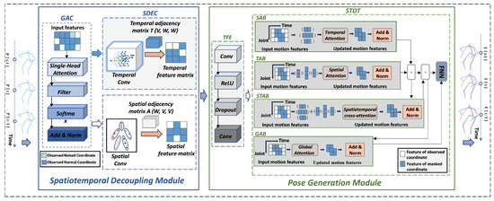
Figure 2.
Our proposed framework via the decoupled spatiotemporal clue: the input historical pose sequence is first processed by the graph attention component (GAC) to dynamically model the spatial dependencies among joints, generating enhanced features. Then, the spatiotemporal decoupling encoding component (SDEC) employs parallel temporal and spatial convolutional branches to separately extract the temporal evolution patterns and spatial structural features, effectively decoupling spatial and temporal information. Subsequently, the temporal feature extractor (TFE) captures local motion dynamics, while the spatiotemporal decoupled transformer (STDT) models the spatial, temporal, cross-dimensional, and global dependencies through four dedicated attention branches (SAB, TAB, STAB, and GAB). Finally, the fused features are passed through a feed-forward Network (FFN) to generate the predicted future pose sequence.
3.1. Spatiotemporal Decoupling Module
As previously discussed, most existing approaches adopt spatiotemporally coupled strategies for modeling human motion encoding. However, the temporal trajectories of different joints often evolve independently, suggesting that coupling spatial and temporal information may result in independent features being overwhelmed by noise, thereby limiting model expressiveness.
To address this issue, we propose the spatiotemporal decoupling module, which aims to model the independence of joint motion trajectories in human pose representations. The module consists of two complementary components: the graph attention component (GAC), and the spatiotemporal decoupling encoding component (SDEC).
Graph Attention Component. Our GAC dynamically learns multi-semantic joint dependencies by introducing an attention mechanism that replaces the fixed skeleton graph used in traditional graph convolutional networks (GCNs), thereby overcoming their limitations in modeling expressive and context-aware features. Unlike static graphs that assume rigid connectivity, our approach enables the adaptive modeling of skeletal topology, where key joints automatically receive higher attention weights based on their topological centrality and functional significance in specific actions. To further improve robustness and physical plausibility, we constructed a dynamic spatial adjacency matrix that facilitates more accurate message passing while suppressing spurious or noisy connections in the graph structure.
Specifically, the dynamic matrix models joint relationships by integrating three components: the static skeleton adjacency matrix , a predefined semantic adjacency matrix , and a learnable semantic adjacency matrix that captures data-driven dependencies. Their combination is nonlinearly transformed via the Sigmoid function to ensure stable gradient propagation:
Here, is a hyperparameter that balances fixed anatomical priors with learned, action-specific relationships (typically set to ). This hybrid design ensures that the learned graph respects fundamental biomechanical constraints while adapting to dynamic motions. After processing the input with GAC, we proceeded to the SDEC for further encoding.
Spatiotemporal Decoupling Encoding Component. The SDEC employs parallel temporal and spatial processing streams. Temporal convolution captures the motion trajectory features along the time dimension, while spatial convolution preserves the kinematic relationships between joints.
Temporal Convolution. Temporal convolution aggregates the motion trajectory features along the time dimension. By treating the channel dimension as a temporal scale, it enables efficient multi-resolution feature extraction over time. Specifically, we define a temporal convolution kernel , where V corresponds to the number of joints and and denote the input and output time steps, respectively. Using Einstein summation notation (Einsum), we combine the input features with the temporal kernel to generate temporal features :
This operation aggregates historical information across time for each joint v, focusing on motion trajectory patterns and effectively encoding temporal dependencies.
Spatial Convolution. The spatial convolution, on the other hand, models the spatial relationships among joints, preserving the biomechanical structure of the human body. Specifically, we define a spatial convolution kernel , which is used to model the spatial relationships between joints. This operation is implemented as a learnable graph convolution that explicitly respects the skeletal topology through a masked adjacency matrix, ensuring that information exchange only occurs between anatomically connected joints.
The effective kernel size is , but it remains sparse due to the structural mask. Padding is not applicable (as this is a graph convolution, i.e., not grid-based). The stride is 1, with full connectivity in the spatial dimension. The key constraint is that only adjacent joints in the skeleton graph are allowed to interact, which enforces kinematic plausibility.
Similarly, using Einsum, we combine the temporally convolved features with the spatial kernel to extract spatial features:
Through this process, we effectively model the spatial topology of the human skeleton and extract meaningful spatial features.
In summary, the SDEC effectively captures diverse spatiotemporal feature relationships through its two complementary components, laying a solid foundation for accurate future pose prediction.
3.2. Pose Generation Module
We propose the pose generation module aims to accurately predict future human pose sequences by separately modeling temporal and spatial dependencies. The module adopts a hierarchical architecture, consisting of two core components: the temporal feature extraction component (TFE), and the spatiotemporally decoupled transformer (STDT).
Temporal Feature Extraction Component. The TFE employs two one-dimensional convolutional kernels with ReLU activation functions, which slide only along the temporal axis without involving the spatial dimension. This design effectively captures the local motion patterns between consecutive frames. Each 1D convolution has a kernel size of 3, a stride of 1, and a padding of 1, ensuring temporal resolution is preserved and local dynamics (e.g., velocity and acceleration) are captured within a short context. The number of input channels is (e.g., 3 for 3D coordinates), and the hidden dimension is set to 64. In this formulation, denotes the hidden state of joint n at time step t, represents the weight matrix associated with time offset , and is the input feature of joint n at time step . The output feature after the first convolution is denoted as , where and are additional learnable weights and bias, respectively. The original input used in the skip connection is represented by . The computational process is defined as follows:
Our design not only filters out high-frequency noise during temporal feature extraction, but it also normalizes local features, providing clean and expressive high-level inputs for the deeper attention mechanisms that follow.
Spatiotemporally Decoupled Transformer. Our STDT is capable of separately modeling the spatial dependencies among joints and their temporal evolution, while simultaneously capturing complex cross-dimensional spatiotemporal dependencies. In contrast to traditional Transformers, we designed four independent attention branches: the spatial attention branch (SAB), the temporal attention branch (TAB), the spatiotemporal cross-Attention branch (STAB), and the global attention branch (GAB). Each attention branch learns its own projection matrices independently, effectively preventing the coupling of spatial and temporal features during parameter updates. Moreover, since the spatial module explicitly models the joint topology, the temporal module can focus solely on dynamic evolution. We argue that single-head attention can act as a “temporal smoother” for spatial features, whereas multi-head attention may introduce redundant or noisy interactions. Therefore, our STDT adopts a single-head attention mechanism. Finally, the fused features are further processed by a feed-forward network (FFN) to produce the final output. We will now provide a detailed description of each component.
Spatial attention branch. In SAB, we compute the self-attention across spatial dimensions within the same time step t. During processing, we divide the TFE outputs into time slices, , and we then compute the query, key, and value as follows:
We share projection weights for keys and values across joints. Notably, in graph-structured data, such as for human skeletons, non-adjacent joints (e.g., left and right feet) typically lack direct mechanical interaction. Hence, we introduce a spatial mask to restrict attention to connected nodes only:
Note that models point-to-point relationships in the spatial dimension S, resulting in a shape in the following form: . Finally, we concatenate all time steps:
Temporal Attention Branch. In TAB, we consider the self-attention across all time steps T within the same spatial point s. Similar to the spatial attention branch, we partition the data by spatial points. Here, a temporal mask ensures that past information does not affect future predictions.
Spatiotemporal cross-attention branch. In STAB, we use spatial attention outputs as queries and temporal attention outputs as keys and values to compute the cross-attention:
For computational efficiency, we reshape the temporal dimension into a single dimension: . To reduce complexity, we apply the spatiotemporal during attention computation:
We reshape the result back to its original form as follows: .
Global attention branch. The GAB flattens all spatiotemporal points to compute the global self-attention, capturing long-range dependencies effectively. After computing all four attention branches, we fuse the features via summation. This ensures that the STDT independently models the spatial dependencies among joints and the temporal evolution of each joint, while capturing complex spatiotemporal interactions. Finally, an FFN produces accurate future human pose sequences.
Our pose generation module is designed not only from the perspective of spatiotemporal decoupling, but it also takes into account both local and global feature modeling. As a shallow network, TFE mainly extracts local features, while the STDT focuses on capturing global features, enabling accurate prediction of future human pose sequences.
3.3. Loss Function
Our loss functions aim to minimize the error between predicted states and target states , and this is followed by SINN (Symplectic INtegral Network) [52]. The loss function is calculated as follows:
where and are the frame-level and node-level weighting factors, which are introduced to prioritize specific frames and nodes during training.
4. Experimental Results
In this section, we comprehensively evaluate our proposed method on two large-scale benchmarks: Human3.6M [22] and AMASS [26].
4.1. Datasets
Human3.6M [22] is the largest benchmark dataset used for evaluating human motion prediction performance. It consists of 15 actions performed by 7 subjects, namely S1, S5, S6, S7, S8, S9, and S11. In this dataset, each human pose is represented by 32 joints to depict the skeletal structure. To ensure fair comparisons with previous works [9,20,21,24,33,53], we follow their protocols by discarding 10 redundant joints (i.e., duplicated joints and global translation points) and retaining 22 joints to represent the human skeleton. Moreover, the frame rate is downsampled from 50 FPS to 25 FPS. Following the testing protocol of Dang et al., Subjects S1, S6, S7, S8, and S9 are used for training; Subject S11 for validation; and Subject S5 for testing.
AMASS [26] is a recently released human motion dataset that aggregates 18 motion capture datasets, including CMU (Carnegie Mellon University motion database), KIT (Karlsruhe Institute of Technology motion dataset), and BMLrub (BML Walking and Running Database from the Max Planck Institute for Intelligent Systems). We selected eight action categories (i.e., playing basketball, basketball signals, directing traffic, jumping, running, playing soccer, walking, and washing windows) to evaluate human motion prediction performance. To ensure fair comparisons with previous works [9,24,53], we removed the global translation joint and redundant joints from the dataset, and we also adopted a 25-joint representation for the human skeleton.
4.2. Comparative Setting
Metrics. We adopted the Mean Per Joint Position Error (MPJPE) as our primary evaluation metric for human motion prediction. MPJPE measures the average Euclidean distance between the predicted and ground-truth joint positions over all J joints and T time steps. A lower MPJPE indicates more accurate predictions. Formally, MPJPE is defined as follows:
where denotes the predicted 3D location of joint j at time t, and is its corresponding ground-truth position.
Baselines. We compared our proposed method with six state-of-the-art (SOTA) methods to comprehensively assess its performance. HisRepItself [8] introduced the innovative concept that future human poses often resemble historical poses using historical information to reconstruct future movements. ProGenIntial [43] proposed a two-stage framework that incrementally refines prediction outputs to align them more closely with the ground truth. CGHMP [53] incorporated additional semantic information to assist the model in predicting future human motion. siMLPe [24] demonstrated that a network consisting solely of fully connected layers could achieve SOTA performance. Lastly, AMHGCN [25] employed four levels of hypergraph representation—joint level, part level, component level, and global level—to comprehensively describe the human skeleton and achieve superior prediction accuracy.
Implementation Details. All experiments were conducted on a single NVIDIA GeForce RTX 4060 GPU with 8 GB of memory. The model was implemented using PyTorch(v2.3.1) [54], and it was trained on an Intel Core i9-13900HX CPU @ 2.20 GHz with 32 GB RAM. We used the Adam optimizer with a batch size of 16 and an initial learning rate of , which decayed by a factor of 0.95 every epoch. Training each model on the Human3.6M dataset took approximately 1.5 h.
4.2.1. Results on Human3.6M
We evaluated our method on Human3.6M for both short-term (≤400 ms) and long-term (>400 ms) motion prediction, and we compared it with six SOTA baselines: HisRepItself [8], ProGenIntial [43], CGHMP [53], PPGMP [23], siMLPe [24], and AMHGCN [25]. As shown in Table 1, our method achieved the best performance in 85 out of 90 prediction scenarios, with near-optimal results in the remaining five (e.g., slight under performance in ‘Walking’ at 80 ms, ‘TakingPhoto’ at 80 ms, and ‘Purchases’ at 160 ms). Crucially, our approach yielded consistent improvements across all actions, as shown in Table 2, achieving an average MPJPE of 94.8 mm at 1000 ms—13.4% lower than the strongest baseline (AMHGCN, 109.5 mm)—validating the claim of a 13% average improvement over the SOTA methods mentioned in the abstract.

Table 1.
Short-term and long-term prediction results on Human3.6M (only selected methods).
Table 2.
Comparison of the average prediction errors (MPJPE) on Human3.6M.
Figure 3 visualizes the predictions for the ‘Eating’ sequence, with ground truth in magenta and predictions in blue–green, and it is annotated with MPJPE values at 80 ms, 400 ms, and 1000 ms. Red dashed rectangles highlight the significant errors. While the baselines performed well in the short term, their predictions drifted over time. In contrast, our method maintained high accuracy throughout, demonstrating superior long-term stability—consistent with the quantitative results.
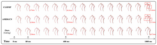
Figure 3.
The qualitative analysis between our proposed DSC and the baselines when applied to the scenario ‘Eating’. From top to bottom, we present the ground truth, as well as the prediction results of CGHMP [53], AMHGCN [25], and our proposed DSC. From left to right, the first pose corresponds to the prediction at 80 ms, the sixth pose is the prediction at 400 ms, and the last pose represents the prediction at 1000 ms. The ground truth is shown in magenta with a solid line, while the comparative results are displayed in blue–green with a solid line. To provide a more intuitive evaluation, we overlaid the corresponding ground truth at each predicted pose location and annotated the MPJPE values at key time points: 80 ms, 400 ms, and 1000 ms. Obvious errors are marked with red dashed rectangles.
To further analyze the performance across motion types, we categorized actions into periodic (e.g., Walking and Eating) and non-periodic/complex (e.g., Discussion, SittingDown, and TakingPhoto) following [36]. As shown in Table 3, our model reduces MPJPE by 23.1% (periodic) and 12.6% (non-periodic) at 1000 ms compared to AMHGCN. This highlights its robustness not only in regular motions, but also in complex, irregular behaviors, indicating strong generalization across diverse temporal and structural patterns.
Table 3.
Comparison of the periodic and non-periodic motion prediction results on Human3.6M (where the MPJPE is in mm, and the lower the value, the better).
4.2.2. Results on AMASS
To further assess the generality and accuracy of our method, we evaluated its performance on the AMASS dataset. Table 4 reports the prediction errors for both short-term (≤400 ms) and long-term (>400 ms) horizons. Our proposed method consistently outperforms all baselines across both prediction lengths, with the performance gap widening in long-term forecasts. These results confirm that our network effectively disentangles the spatial and temporal motion features from the input historical sequence, enabling the precise prediction of future human poses.
Table 4.
Comparison of the average prediction errors (MPJPE) on AMASS.
4.2.3. Computational Efficiency
We evaluated the computational efficiency of our method to assess its suitability for real-time applications. We compared our approach with key baselines: CGHMP [53], siMLPe [24], and AMHGCN [25]. All experiments were conducted on a single NVIDIA GeForce RTX 4060 GPU (8 GB VRAM) using a 25-frame input sequence (625 ms at 40 Hz). Results were averaged over 1000 forward passes on the Human3.6M test set.
Table 5 reports the model parameters (in millions), FLOPs (in G), inference latency (in ms), GPU memory usage (in MB), and approximate training time per run. Our method achieved a latency of 13.9 ms, or about 72 FPS, meeting the requirements for real-time use in AR/VR, robotics, and animation. This is faster than AMHGCN (13.4 ms) and only slightly slower than siMLPe (9.1 ms), which has lower computational demands but weaker accuracy (see Section 4.2.1).
Table 5.
Computational efficiency comparison on Human3.6M. Lower values are better for all metrics except FPS (where higher is better).
Our model has 2 M parameters, making it more compact than CGHMP (4.9 M) and reasonably lightweight overall. While our FLOPs (0.7 G) are higher than siMLPe (0.1 G) and AMHGCN (0.2 G), this reflects the cost of explicit temporal modeling through disentangled spatiotemporal pathways. Despite this, our GPU memory footprint (1110 MB) is moderate and lower than CGHMP (1320 MB), indicating efficient memory utilization. Training converges in approximately 1.5 h, faster than CGHMP (1.8 h) and comparable to siMLPe (1.2 h) and AMHGCN (1.3 h). The efficient training is attributed to stable gradient flow and reduced feature entanglement due to the decoupled architecture design.
In summary, our method achieves a strong balance between accuracy and efficiency. It offers competitive inference speed, moderate resource usage, and fast training, while maintaining a compact model size. These characteristics make it practical for both research and real-world deployment.
4.3. Decoupling Spatiotemporal Experiment
To empirically evaluate the effectiveness of explicit spatiotemporal decoupling, we designed four configurations that selectively remove or weaken the decoupling mechanism: (1) No-Decoupling Encoder, which replaces the disentangled encoder with a standard joint spatiotemporal model, forcing spatial and temporal features to be learned jointly; (2) Multi-Head Generator, which employs multi-head self-attention in the generation module—instead of the proposed single-head temporal smoother—and may introduce redundant cross-joint interactions; (3) Fully Coupled Baseline, which removes spatiotemporal separation in both the encoder and generator, representing a conventional end-to-end architecture; and (4) Decoupled Full Model, which retains both the disentangled encoder and the single-head attention generator, corresponding to the complete proposed framework. This comparative study enables us to assess how varying levels of decoupling influence the overall prediction performance.
As shown in Table 6, all models without full decoupling suffer performance degradation, especially in long-term predictions. The fully coupled baseline performed the worst, with the average MPJPE increasing from 47.8 mm to 69.7 mm, which represents an increase of over 45%. This sharp decline suggests that entangled modeling obscures the critical kinematic patterns under complex motion dynamics. Even partial removal of decoupling, such as using multi-head attention in the generation module, leads to noticeable error growth at longer horizons. For example, the prediction error at 1000 ms rises significantly compared to the full model, indicating that excessive interaction modeling harms temporal consistency. In contrast, the fully decoupled model exhibits the most stable error progression, demonstrating superior generalization and reduced error accumulation over time.
Table 6.
Comparison of spatiotemporal decoupling in the pose encoding and generation modules.
These results demonstrate that explicit spatiotemporal decoupling is not merely beneficial but essential for accurate and stable motion prediction. By preventing feature entanglement and allowing specialized modeling of spatial topology and temporal dynamics, our design enables more reliable long-term forecasting—particularly under autoregressive settings where error accumulation is a major challenge.
4.4. Ablation Studies
In this section, we present a systematic ablation study that was conducted on the two core modules of our proposed method: the Spatiotemporal Decoupling Module (SDM), and the Pose Generation Module (PGM). The SDM performs disentangled encoding of human poses by separately modeling spatial and temporal feature relationships. The PGM accurately predicts future pose sequences by independently modeling temporal and spatial dependencies. The spatiotemporal decoupling module consists of two components: the graph attention component (GAC), and the spatiotemporal decoupling encoding component (SDEC). The PGM also comprises two key components: the temporal feature extraction (TFE) component, and the spatiotemporally decoupled transformer (STDT).
To evaluate the contribution of each key component to the overall performance, we designed four plug-and-play ablation settings: (1) removing the GAC; (2) replacing the TFE module with a standard TCN; (3) substituting the STDT with a conventional Transformer architecture; and (4) replacing the SDEC encoder with a standard GCN. These ablation studies help us better understand the role and effectiveness of each individual component in the proposed framework.
The results in Table 7 show that all ablation settings lead to performance degradation, confirming that each component contributes meaningfully to the final accuracy. Notably, replacing SDEC with a standard GCN results in the largest performance drop, with the average MPJPE increasing from 47.8 mm to 61.5 mm. This highlights the limitations of joint spatiotemporal modeling, which tends to introduce feature entanglement and impair prediction accuracy. Similarly, substituting STDT with a standard Transformer leads to a substantial increase in long-term prediction errors, particularly at the 1000 ms horizon. This suggests that entangled attention mechanisms are prone to error accumulation over time. Removing the GAC component results in an average MPJPE of 59.5 mm, with noticeable degradation in mid-term predictions. This indicates that the GAC not only enhances spatial feature learning through adaptive attention, but that it also helps preserve biomechanical plausibility by reinforcing anatomically meaningful joint dependencies and suppressing physically implausible connections during message passing.
Table 7.
Ablation study on the components of human motion prediction via the decoupled spatiotemporal clue network.
The full model achieves the lowest MPJPE across all horizons, validating the effectiveness of our decoupled design. These results collectively demonstrate that explicit separation of spatial and temporal modeling is not only beneficial, but also essential for accurate and stable long-term human motion prediction.
5. Discussion
Our method achieves SOTA performance in 3D human motion prediction on the Human3.6M and AMASS benchmarks. The proposed spatiotemporal decoupling enables independent yet complementary modeling of joint kinematics (spatial topology) and motion dynamics (temporal evolution), validating our hypothesis that disentangled representation learning mitigates error propagation and improves long-term stability. Compared to recent SOTA methods, such as siMLPe and AMHGCN, our model shows consistent reductions in MPJPE, especially at longer horizons (e.g., 600–1000 ms), indicating effective suppression of error accumulation in autoregressive generation. The explicit disentanglement of spatial and temporal factors not only boosts prediction accuracy, but also enhances model interpretability—enabling the diagnosis of spatial versus temporal error sources—and it supports modular designs for downstream applications.
Despite these advances, several limitations remain. First, the model relies on a fixed skeletal graph learned from a canonical skeleton, limiting generalization across subjects with varying body proportions (e.g., limb lengths). This constraint may hinder deployment in personalized domains, such as clinical gait analysis or prosthetic control, where subject-specific biomechanics are critical. Second, while the decoupled architecture improves accuracy, it increases model complexity and parameter count compared to unified end-to-end designs, potentially affecting inference speed and memory footprint—challenging real-time use in mobile robotics or AR/VR. Moreover, training on studio-collected datasets (e.g., Human3.6M) under controlled conditions may compromise robustness to real-world variations, such as clothing, occlusion, or outdoor motion patterns.
Future work will address these challenges through several principled directions. (1) Adaptive graph learning: Exploring dynamic graph neural networks (e.g., EvolveGCN) or attention-based adjacency adaptation to model subject-specific skeletons; (2) Physical plausibility: Integrating biomechanical constraints (e.g., joint limits and self-collision avoidance) and dynamic smoothness priors (e.g., jerk minimization) into the loss or inference pipeline; (3) Controllable generation: Extending the framework to support multimodal prediction (via stochastic latent variables) and interactive synthesis (conditioning on goals or environmental cues); (4) Cross-dataset generalization: Investigating domain-invariant representations and unsupervised alignment techniques (e.g., via contrastive learning or adversarial adaptation) to enable transfer across datasets with different capture protocols, sensor types, or annotation styles; (5) Few-shot and zero-shot adaptation: Designing meta-learning or prompt-based mechanisms to rapidly adapt the model to new subjects or actions with minimal labeled data, leveraging the disentangled structure for efficient parameter reuse. (6) Physics-aware interactive generation via reinforcement learning: Integrate physics engines (e.g., MuJoCo and Bullet) with reinforcement learning to enable physically plausible and goal-driven motion synthesis. By training RL agents within a simulated environment governed by physical laws (e.g., gravity and contact dynamics), our model can generate motions that are not only kinematically accurate, but also dynamically realistic and responsive to user commands or environmental constraints (e.g., obstacle avoidance and target reaching).
These extensions aim to build more realistic, personalized, and adaptive motion prediction systems—advancing toward a systems science perspective that emphasizes modularity, transferability, and robust co-design across diverse environments and users. Such capabilities are essential for next-generation applications in assistive robotics, digital avatars, and human-AI collaboration.
6. Conclusions
In this paper, we present a novel framework for 3D human motion prediction based on explicit spatiotemporal disentanglement. The method consists of two core modules: (1) a spatiotemporal decoupling module that separately models spatial kinematics (bone lengths, joint connectivity, etc.) and temporal dynamics (motion trajectories), and (2) a pose generation module that synthesizes future poses by integrating decoupled spatial and temporal features. This design enables more stable long-term prediction by reducing error propagation across entangled dimensions.
Our work presents a principled framework for disentangled spatiotemporal modeling, offering new insights into the design of interpretable and modular architectures for human motion prediction. By decoupling spatial and temporal factors, we achieve more accurate, stable, and reproducible long-term forecasting. This approach lays the foundation for future systems that are not only predictive, but also physically plausible, personalized, and controllable key requirements for real-world deployment in robotics, virtual avatars, and human-centered AI.
Author Contributions
Conceptualization, M.X. and E.L.; methodology, M.X.; software, M.X.; validation, M.X.; formal analysis, M.X.; investigation, M.X.; data curation, M.X.; writing—original draft preparation, M.X.; writing—review and editing, Z.G.; visualization, M.X.; supervision, E.L.; project administration, E.L. All authors have read and agreed to the published version of the manuscript.
Funding
This research received no external funding.
Institutional Review Board Statement
Not applicable.
Informed Consent Statement
Not applicable.
Data Availability Statement
The data presented in this study are available in two publicly accessible datasets: the Human3.6M dataset (http://vision.imar.ro/human3.6m/description.php, accessed on 24 November 2024), and the AMASS dataset (https://amass.is.tue.mpg.de/, accessed on 15 March 2025)). These datasets were used for training and evaluating the proposed 3D human motion prediction model. No new data were generated in this study.
Acknowledgments
We wish to thank the teams behind the Human3.6M and AMASS datasets for their publicly available motion data. Computational resources were provided by the High-Performance Computing Platform at Tsinghua University.
Conflicts of Interest
The authors declare no conflicts of interest.
References
- Lyu, K.; Chen, H.; Liu, Z.; Zhang, B.; Wang, R. 3D Human Motion Prediction: A Survey. Neurocomputing 2022, 489, 345–365. [Google Scholar] [CrossRef]
- Troje, N.F. Decomposing Biological Motion: A Framework for Analysis and Synthesis of Human Gait Patterns. J. Vis. 2002, 2, 2. [Google Scholar] [CrossRef] [PubMed]
- Liu, X.; Yin, J.; Liu, J.; Ding, P.; Liu, J.; Liu, H. TrajectoryCNN: A New Spatio-Temporal Feature Learning Network for Human Motion Prediction. IEEE Trans. Circuits Syst. Video Technol. 2021, 31, 2133–2146. [Google Scholar] [CrossRef]
- Koppula, H.S.; Saxena, A. Anticipating Human Activities for Reactive Robotic Response. In Proceedings of the 2013 IEEE/RSJ International Conference on Intelligent Robots and Systems (IROS), Tokyo, Japan, 3–7 November 2013; IEEE: Piscataway, NJ, USA, 2013; pp. 4476–4483. [Google Scholar]
- Unhelkar, V.V.; Lasota, P.A.; Tyroller, Q.; Buhai, R.-D.; Marceau, L.; Deml, B.; Shah, J.A. Human-Aware Robotic Assistant for Collaborative Assembly: Integrating Human Motion Prediction with Planning in Time. IEEE Robot. Autom. Lett. 2018, 3, 2394–2401. [Google Scholar] [CrossRef]
- Cao, Z.; Gao, H.; Mangalam, K.; Cai, Q.-Z.; Vo, M.; Malik, J. Long-Term Human Motion Prediction with Scene Context. In Computer Vision—ECCV 2020, Proceedings of the 16th European Conference on Computer Vision, Glasgow, UK, 23–28 August 2020; Proceedings, Part I; Vedaldi, A., Bischof, H., Brox, T., Frahm, J.-M., Eds.; Springer: Cham, Switzerland, 2020; pp. 387–404. [Google Scholar]
- Sofianos, T.; Sampieri, A.; Franco, L.; Galasso, F. Space-Time-Separable Graph Convolutional Network for Pose Forecasting. In Proceedings of the IEEE/CVF International Conference on Computer Vision (ICCV), Montreal, QC, Canada, 10–17 October 2021; IEEE: Piscataway, NJ, USA, 2021; pp. 11209–11218. [Google Scholar]
- Mao, W.; Liu, M.; Salzmann, M. History Repeats Itself: Human Motion Prediction via Motion Attention. In Computer Vision—ECCV 2020, Proceedings of the 16th European Conference on Computer Vision, Glasgow, UK, 23–28 August 2020; Proceedings, Part XIV; Bartoli, A., Fusiello, A., Eds.; Springer: Cham, Switzerland, 2020; pp. 474–489. [Google Scholar]
- Mao, W.; Liu, M.; Salzmann, M.; Li, H. Learning Trajectory Dependencies for Human Motion Prediction. In Proceedings of the IEEE/CVF International Conference on Computer Vision (ICCV), Seoul, Republic of Korea, 27 October–2 November 2019; IEEE: Piscataway, NJ, USA, 2019; pp. 9489–9497. [Google Scholar]
- Wang, B.; Adeli, E.; Chiu, H.-K.; Huang, D.-A.; Niebles, J.C. Imitation Learning for Human Pose Prediction. In Proceedings of the IEEE/CVF International Conference on Computer Vision (ICCV), Seoul, Republic of Korea, 27 October–2 November 2019; IEEE: Piscataway, NJ, USA, 2019; pp. 7124–7133. [Google Scholar]
- Chiu, H.-K.; Adeli, E.; Wang, B.; Huang, D.-A.; Niebles, J.C. Action-Agnostic Human Pose Forecasting. In Proceedings of the 2019 IEEE Winter Conference on Applications of Computer Vision (WACV), Waikoloa, HI, USA, 7–11 January 2019; IEEE: Piscataway, NJ, USA, 2019; pp. 1423–1432. [Google Scholar]
- Adeli, V.; Adeli, E.; Reid, I.; Niebles, J.C.; Rezatofighi, H. Socially and Contextually Aware Human Motion and Pose Forecasting. IEEE Robot. Autom. Lett. 2020, 5, 6033–6040. [Google Scholar] [CrossRef]
- Yuan, Y.; Kitani, K.M. DLow: Diversifying Latent Flows for Diverse Human Motion Prediction. In Computer Vision—ECCV 2020, Proceedings of the 16th European Conference on Computer Vision, Glasgow, UK, 23–28 August 2020; Proceedings, Part IX; Bolec, G., Corso, G., Fusiello, A., Eds.; Springer: Cham, Switzerland, 2020; pp. 346–364. [Google Scholar]
- Yuan, Y.; Kitani, K.M. Ego-Pose Estimation and Forecasting as Real-Time PD Control. In Proceedings of the IEEE/CVF International Conference on Computer Vision (ICCV), Seoul, Republic of Korea, 27 October–2 November 2019; IEEE: Piscataway, NJ, USA, 2019; pp. 10082–10092. [Google Scholar]
- Aksan, E.; Kaufmann, M.; Cao, P.; Hilliges, O. A Spatio-Temporal Transformer for 3D Human Motion Prediction. In Proceedings of the 2021 International Conference on 3D Vision (3DV), Montréal, QC, Canada, 1–3 November 2021; IEEE: Piscataway, NJ, USA, 2021; pp. 565–574. [Google Scholar]
- Xu, C.; Tan, R.T.; Tan, Y.; Chen, S.; Wang, X.; Wang, Y. Auxiliary Tasks Benefit 3D Skeleton-Based Human Motion Prediction. In Proceedings of the IEEE/CVF International Conference on Computer Vision (ICCV), Paris, France, 2–6 October 2023; IEEE: Piscataway, NJ, USA, 2023; pp. 9509–9520. [Google Scholar]
- Cao, W.; Li, S.; Zhong, J. A Dual Attention Model Based on Probabilistically Mask for 3D Human Motion Prediction. Neurocomputing 2022, 493, 106–118. [Google Scholar] [CrossRef]
- von Marcard, T.; Henschel, R.; Black, M.J.; Rosenhahn, B.; Pons-Moll, G. Recovering Accurate 3D Human Pose in the Wild Using IMUs and a Moving Camera. In Proceedings of the European Conference on Computer Vision (ECCV), Munich, Germany, 8–14 September 2018; Springer: Cham, Switzerland, 2018; pp. 601–617. [Google Scholar]
- Ding, P.; Yin, J. Towards More Realistic Human Motion Prediction with Attention to Motion Coordination. IEEE Trans. Circuits Syst. Video Technol. 2022, 32, 5846–5858. [Google Scholar] [CrossRef]
- Li, M.; Chen, S.; Zhao, Y.; Zhang, Y.; Wang, Y.; Tian, Q. Dynamic Multiscale Graph Neural Networks for 3D Skeleton Based Human Motion Prediction. In Proceedings of the IEEE/CVF Conference on Computer Vision and Pattern Recognition (CVPR), Seattle, WA, USA, 13–19 June 2020; IEEE: Piscataway, NJ, USA, 2020; pp. 214–223. [Google Scholar]
- Dang, L.; Nie, Y.; Long, C.; Zhang, Q.; Li, G. MSR-GCN: Multi-Scale Residual Graph Convolution Networks for Human Motion Prediction. In Proceedings of the IEEE/CVF International Conference on Computer Vision (ICCV), Montreal, QC, Canada, 10–17 October 2021; IEEE: Piscataway, NJ, USA, 2021; pp. 11467–11476. [Google Scholar]
- Ionescu, C.; Papava, D.; Olaru, V.; Sminchisescu, C. Human3.6M: Large Scale Datasets and Predictive Methods for 3D Human Sensing in Natural Environments. IEEE Trans. Pattern Anal. Mach. Intell. 2013, 36, 1325–1339. [Google Scholar] [CrossRef] [PubMed]
- Li, J.; Wang, J.; Kuang, C.; Wu, L.; Wang, X.; Xu, Y. A Human-Like Action Learning Process: Progressive Pose Generation for Motion Prediction. Knowl.-Based Syst. 2023, 280, 110948. [Google Scholar] [CrossRef]
- Guo, W.; Du, Y.; Shen, X.; Lepetit, V.; Alameda-Pineda, X.; Moreno-Noguer, F. Back to MLP: A Simple Baseline for Human Motion Prediction. In Proceedings of the IEEE/CVF Winter Conference on Applications of Computer Vision (WACV), Waikoloa, HI, USA, 4–8 January 2023; IEEE: Piscataway, NJ, USA, 2023; pp. 4809–4819. [Google Scholar]
- Li, J.; Wang, J.; Wu, L.; Wang, X.; Luo, X.; Xu, Y. AMHGCN: Adaptive Multi-Level Hypergraph Convolution Network for Human Motion Prediction. Neural Netw. 2024, 172, 110948. [Google Scholar] [CrossRef] [PubMed]
- Mahmood, N.; Ghorbani, N.; Troje, N.F.; Pons-Moll, G.; Black, M.J. AMASS: Archive of Motion Capture as Surface Shapes. In Proceedings of the IEEE/CVF International Conference on Computer Vision (ICCV), Seoul, Republic of Korea, 27 October–2 November 2019; IEEE: Piscataway, NJ, USA, 2019; pp. 5442–5451. [Google Scholar]
- Wang, J.; Hertzmann, A.; Fleet, D.J. Gaussian Process Dynamical Models. In Proceedings of the Advances in Neural Information Processing Systems (NeurIPS 2005), Vancouver, BC, Canada, 5–8 December 2005; MIT Press: Cambridge, MA, USA, 2005; Volume 18. [Google Scholar]
- Taylor, G.W.; Hinton, G.E.; Roweis, S. Modeling Human Motion Using Binary Latent Variables. In Proceedings of the Advances in Neural Information Processing Systems (NeurIPS 2006), Vancouver, BC, Canada, 4–7 December 2006; MIT Press: Cambridge, MA, USA, 2006; Volume 19. [Google Scholar]
- Brand, M.; Hertzmann, A. Style Machines. In Proceedings of the 27th Annual Conference on Computer Graphics and Interactive Techniques (SIGGRAPH 2000), New Orleans, LA, USA, 23–28 July 2000; ACM: New York, NY, USA; Addison-Wesley: Boston, MA, USA, 2000; pp. 183–192. [Google Scholar]
- Lehrmann, A.M.; Gehler, P.V.; Nowozin, S. Efficient Nonlinear Markov Models for Human Motion. In Proceedings of the IEEE Conference on Computer Vision and Pattern Recognition (CVPR), Columbus, OH, USA, 23–28 June 2014; IEEE: Piscataway, NJ, USA, 2014; pp. 1314–1321. [Google Scholar]
- Pavlovic, V.; Rehg, J.M.; MacCormick, J. Learning Switching Linear Models of Human Motion. In Proceedings of the Advances in Neural Information Processing Systems (NeurIPS 2000), Denver, CO, USA, 30 November–3 December 2000; MIT Press: Cambridge, MA, USA, 2000; Volume 13. [Google Scholar]
- Fragkiadaki, K.; Levine, S.; Felsen, P.; Malik, J. Recurrent Network Models for Human Dynamics. In Proceedings of the IEEE International Conference on Computer Vision (ICCV), Santiago, Chile, 7–13 December 2015; IEEE: Piscataway, NJ, USA, 2015; pp. 4346–4354. [Google Scholar]
- Martinez, J.; Black, M.J.; Romero, J. On Human Motion Prediction Using Recurrent Neural Networks. In Proceedings of the IEEE Conference on Computer Vision and Pattern Recognition (CVPR), Honolulu, HI, USA, 21–26 July 2017; IEEE: Piscataway, NJ, USA, 2017; pp. 2891–2900. [Google Scholar]
- Cui, Q.; Sun, H.; Kong, Y.; Zhang, X.; Li, Y. Efficient Human Motion Prediction Using Temporal Convolutional Generative Adversarial Network. Inf. Sci. 2021, 545, 427–447. [Google Scholar] [CrossRef]
- Gui, L.-Y.; Wang, Y.-X.; Liang, X.; Moura, J.M.F. Adversarial Geometry-Aware Human Motion Prediction. In Proceedings of the European Conference on Computer Vision (ECCV), Munich, Germany, 8–14 September 2018; Springer: Cham, Switzerland, 2018; pp. 786–803. [Google Scholar]
- Li, C.; Zhang, Z.; Lee, W.S.; Lee, G.H. Convolutional Sequence to Sequence Model for Human Dynamics. In Proceedings of the IEEE Conference on Computer Vision and Pattern Recognition (CVPR), Salt Lake City, UT, USA, 18–23 June 2018; IEEE: Piscataway, NJ, USA, 2018; pp. 5226–5234. [Google Scholar]
- Butepage, J.; Black, M.J.; Kragic, D.; Kjellström, H. Deep Representation Learning for Human Motion Prediction and Classification. In Proceedings of the IEEE Conference on Computer Vision and Pattern Recognition (CVPR), Honolulu, HI, USA, 21–26 July 2017; IEEE: Piscataway, NJ, USA, 2017; pp. 6158–6166. [Google Scholar]
- Yang, H.; Yuan, C.; Zhang, L.; Sun, Y.; Hu, W.; Maybank, S.J. STA-CNN: Convolutional Spatial-Temporal Attention Learning for Action Recognition. IEEE Trans. Image Process. 2020, 29, 5783–5793. [Google Scholar] [CrossRef] [PubMed]
- Lea, C.; Flynn, M.D.; Vidal, R.; Reiter, A.; Hager, G.D. Temporal Convolutional Networks for Action Segmentation and Detection. In Proceedings of the IEEE Conference on Computer Vision and Pattern Recognition (CVPR), Honolulu, HI, USA, 21–26 July 2017; IEEE: Piscataway, NJ, USA, 2017; pp. 156–165. [Google Scholar]
- Bai, S.; Kolter, J.Z.; Koltun, V. An Empirical Evaluation of Generic Convolutional and Recurrent Networks for Sequence Modeling. arXiv 2018, arXiv:1803.01271. [Google Scholar] [CrossRef]
- Huang, J.; Kang, H. 3D Skeleton-Based Human Motion Prediction Using Spatial–Temporal Graph Convolutional Network. Int. J. Multimed. Inf. Retr. 2024, 13, 33. [Google Scholar] [CrossRef]
- Cui, Q.; Sun, H.; Yang, F. Learning Dynamic Relationships for 3D Human Motion Prediction. In Proceedings of the IEEE/CVF Conference on Computer Vision and Pattern Recognition (CVPR), Virtual, 13–19 June 2020; IEEE: Piscataway, NJ, USA, 2020; pp. 6519–6527. [Google Scholar]
- Ma, T.; Nie, Y.; Long, C.; Zhang, Q.; Li, G. Progressively Generating Better Initial Guesses towards Next Stages for High-Quality Human Motion Prediction. In Proceedings of the IEEE/CVF Conference on Computer Vision and Pattern Recognition (CVPR), New Orleans, LA, USA, 19–24 June 2022; IEEE: Piscataway, NJ, USA, 2022; pp. 6437–6446. [Google Scholar]
- Paden, B.; Čáp, M.; Yong, S.Z.; Yershov, D.; Frazzoli, E. A Survey of Motion Planning and Control Techniques for Self-Driving Urban Vehicles. IEEE Trans. Intell. Veh. 2016, 1, 33–55. [Google Scholar] [CrossRef]
- Cho, K.; Van Merriënboer, B.; Gulcehre, C.; Bahdanau, D.; Bougares, F.; Schwenk, H.; Bengio, Y. Learning Phrase Representations Using RNN Encoder-Decoder for Statistical Machine Translation. arXiv 2014, arXiv:1406.1078. [Google Scholar] [CrossRef]
- Yan, S.; Xiong, Y.; Lin, D. Spatial Temporal Graph Convolutional Networks for Skeleton-Based Action Recognition. In Proceedings of the AAAI Conference on Artificial Intelligence (AAAI-18), New Orleans, LA, USA, 2–7 February 2018; AAAI Press: Palo Alto, CA, USA, 2018; Volume 32. [Google Scholar]
- Zhao, R.; Su, H.; Ji, Q. Bayesian Adversarial Human Motion Synthesis. In Proceedings of the IEEE/CVF Conference on Computer Vision and Pattern Recognition (CVPR), Virtual, 13–19 June 2020; IEEE: Piscataway, NJ, USA, 2020; pp. 6225–6234. [Google Scholar]
- Cui, Q.; Sun, H. Towards Accurate 3D Human Motion Prediction from Incomplete Observations. In Proceedings of the IEEE/CVF Conference on Computer Vision and Pattern Recognition (CVPR), Nashville, TN, USA, 10–17 June 2021; IEEE: Piscataway, NJ, USA, 2021; pp. 4801–4810. [Google Scholar]
- Martínez-González, A.; Villamizar, M.; Odobez, J.-M. Pose Transformers (PoTR): Human Motion Prediction with Non-Autoregressive Transformers. In Proceedings of the IEEE/CVF International Conference on Computer Vision (ICCV), Montreal, QC, Canada, 10–17 October 2021; IEEE: Piscataway, NJ, USA, 2021; pp. 2276–2284. [Google Scholar]
- Hua, Y.; Xuanzhe, F.; Yaqing, H.; Liu, Y.; Cai, K.; Dongsheng, Z.; Qiang, Z. Towards Efficient 3D Human Motion Prediction Using Deformable Transformer-Based Adversarial Network. In Proceedings of the 2022 International Conference on Robotics and Automation (ICRA), Philadelphia, PA, USA, 30 May–5 June 2022; IEEE: Piscataway, NJ, USA, 2022; pp. 861–867. [Google Scholar]
- Cai, Y.; Huang, L.; Wang, Y.; Cham, T.-J.; Cai, J.; Yuan, J.; Liu, J.; Yang, X.; Zhu, Y.; Shen, X.; et al. Learning Progressive Joint Propagation for Human Motion Prediction. In Computer Vision—ECCV 2020, Proceedings of the 16th European Conference on Computer Vision, Glasgow, UK, 23–28 August 2020; Proceedings, Part VII; Springer: Cham, Switzerland, 2020; pp. 226–242. [Google Scholar]
- Chen, H.; Lyu, K.; Liu, Z.; Yin, Y.; Yang, X.; Lyu, Y. Rethinking Human Motion Prediction with Symplectic Integral. In Proceedings of the IEEE/CVF Conference on Computer Vision and Pattern Recognition (CVPR), Seattle, WA, USA, 16–22 June 2024; IEEE: Piscataway, NJ, USA, 2024; pp. 2134–2143. [Google Scholar]
- Li, J.; Pan, H.; Wu, L.; Huang, C.; Luo, X.; Xu, Y. Class-Guided Human Motion Prediction via Multi-Spatial-Temporal Supervision. Neural Comput. Appl. 2023, 35, 9463–9479. [Google Scholar] [CrossRef]
- Paszke, A.; Gross, S.; Massa, F.; Bradbury, J.; Chanan, G.; Killeen, T.; Lin, Z.; Gimelshein, N.; Antiga, L.; Desmaison, A.; et al. PyTorch: An Imperative Style, High-Performance Deep Learning Library. In Proceedings of the Advances in Neural Information Processing Systems 32 (NeurIPS), Vancouver, BC, Canada, 8–14 December 2019; pp. 8026–8037. [Google Scholar]


Disclaimer/Publisher’s Note: The statements, opinions and data contained in all publications are solely those of the individual author(s) and contributor(s) and not of MDPI and/or the editor(s). MDPI and/or the editor(s) disclaim responsibility for any injury to people or property resulting from any ideas, methods, instructions or products referred to in the content. |
© 2025 by the authors. Licensee MDPI, Basel, Switzerland. This article is an open access article distributed under the terms and conditions of the Creative Commons Attribution (CC BY) license (https://creativecommons.org/licenses/by/4.0/).