Abstract
The objective of this study is to determine the optimal machine learning model for constructing electric field strength maps across urban areas, advancing the field of environmental monitoring. These models are unique because they use a detailed dataset that goes beyond electromagnetic readings, incorporating information like population density, urbanization levels, and building characteristics. This novel approach, combined with explainable AI, helps identify the key factors affecting electromagnetic exposure. The models enable the creation of highly detailed and dynamic maps of electromagnetic pollution. These maps are not just static snapshots, they can track changes over time, evaluate the success of mitigation efforts, and provide deeper insights into how electromagnetic fields are distributed in urban areas. To construct a detailed electric field strength map, we conducted an extensive analysis using 410 machine learning models across the urban area of Paris, incorporating three fundamental approaches: k-nearest neighbors, neural networks, and decision trees. This comprehensive exploration allowed us to evaluate and optimize various model configurations, ensuring robust and accurate predictions of electric field strength across diverse urban environments. The kNN model exhibited the most consistent performance, with an RMSE of and an SD of . The analysis indicates that kNN outperforms simple neural networks and decision trees in terms of both RMSE and performance stability. From the SHAP analysis, we conclude that the feature representing the total volume of buildings in the area around each antenna (V) is the most significant in predicting electromagnetic field strength in the kNN regression model, consistently showing a high impact across predictions. The population density feature (POP) also demonstrates considerable influence.
1. Introduction
1.1. The Motivation
The strength of the electric field and its potential health effects, particularly concerning radio frequency (RF) and nonionizing radiation, remain subjects of ongoing research [1,2]. Electric fields can generate currents within the human body, and while low levels are generally considered harmless, higher levels associated with exposure to RF and microwaves can result in tissue heating [3,4]. The potential link between long-term high-level exposure to RF and cancer, especially brain tumors, continues to be the focus of active study [5]. The International Agency for Research on Cancer (IARC) has classified RF electromagnetic fields as “possibly carcinogenic to humans” (Group 2B). Furthermore, research suggests a possible association between exposure to electromagnetic fields (EMFs) and neurological problems such as headaches, sleep disturbances, and cognitive impairment, although the evidence remains inconclusive [6]. Some individuals report symptoms such as headaches, fatigue, and stress, which they attribute to exposure to EMF. Although the World Health Organization (WHO) does not recognize electromagnetic hypersensitivity (EHS) as a medical diagnosis, the reported symptoms are real and can be severe for those affected. Regulatory organizations, including the International Commission on Non-Ionizing Radiation Protection (ICNIRP) and the Federal Communications Commission (FCC), have established safety guidelines for exposure based on scientific evidence. These guidelines are periodically reviewed to incorporate new research findings [7]. The expansion of 5G technology has also raised public concerns about its potential health impacts [8,9]. Consequently, public health agencies continue to emphasize the need for ongoing research into the long-term health effects of RF exposure and advocate for evidence-based guidelines to ensure public safety.
1.2. Objectives
Understanding the connection between electric field strength and health requires continuous research and monitoring. This ensures safe exposure limits and mitigates potential risks through informed regulations and public awareness. Many cities lack detailed maps of electric field strength, which hinders informed decision making. This research addresses this gap by pioneering a novel machine learning (ML) approach. Our method goes beyond simply predicting or estimating electromagnetic field strength; it utilizes explainable artificial intelligence (XAI) to provide valuable insights. The key lies in our comprehensive dataset. It incorporates not only field strength measurements, but also crucial factors such as population density, urbanization levels, and detailed building information. We trained various ML models, including k-nearest neighbors, neural networks, and decision trees, on this rich dataset to create highly accurate electric field strength maps. But the value extends beyond the map itself. Using XAI, we can understand how these urban elements influence electromagnetic exposure. This transparency empowers city planners, policymakers, and researchers. They gain a deeper understanding of the relationship between urban infrastructure and electromagnetic field distribution, enabling them to make informed decisions for safer and more sustainable urban environments.
Our research on predicting electric field strength in urban areas is groundbreaking for the following reasons:
- By leveraging explainable AI, our models do more than just estimate electric field strength; they reveal the key urban factors—such as population density, building characteristics, and urbanization levels—that most significantly influence electric field strength. This transparency fosters trust in the models and facilitates their practical application.
- Our unique dataset goes beyond traditional field strength measurements. It incorporates rich geographical features, providing a holistic view of the electric field distribution. This comprehensive approach sets a new standard for the accuracy of prediction.
- Our research generates detailed electric field strength maps for large urban areas. These maps are not only informative, they are actionable tools. They empower individuals, organizations, and policymakers to make informed decisions about urban planning, public health initiatives, and proactive risk management strategies.
- Understanding these key determinants empowers policymakers to develop targeted and effective interventions. This can include crafting regulations or urban design strategies that mitigate potential risks associated with RF radiation.
1.3. Related Work
Scientific research on the levels of exposure to radiofrequency (RF) electromagnetic fields and radiofrequency electromagnetic fields (RF-EMFs) in both outdoor and indoor environments has seen significant advancements in recent years [10,11,12]. This emerging field has attracted considerable attention due to the widespread proliferation of wireless communication devices and the growing public concern about potential health risks [13,14]. Studies have increasingly focused on understanding the spatial distribution and temporal variation of RF-EMF exposure, employing advanced measurement techniques and sophisticated modeling approaches [15,16,17]. Researchers not only map exposure levels in diverse environments but also investigate the implications of prolonged exposure on human health, thus contributing to the development of more effective safety standards and guidelines.
The body of literature on the application of machine learning for electromagnetic field strength estimation is relatively limited. Therefore, we will highlight the most relevant and significant works identified in our review. In [18], the authors investigated the mapping of electromagnetic field (EMF) exposure from cellular base station antennas (BSAs) using artificial neural networks (ANNs). The EMF exposure map (EEM) in urban areas is created using data from EMF sensor networks, drive tests, and public databases that detail the locations and orientations of the BSAs. In addition, in [19], the researchers explored the use of artificial neural networks (ANNs) for the spatial reconstruction of exposure to radiofrequency electromagnetic fields (RF-EMFs) in an outdoor urban environment. They conducted drive test measurement campaigns that covered approximately 65 km in Paris, recording electric field strength (E) across a wide band from 700 to 2700 MHz. Furthermore, ref. [20] aimed to accurately reconstruct electromagnetic field exposure maps in urban areas using limited sensor data. By training a model on environmental factors, the authors effectively predicted field propagation and generated detailed exposure maps in a short area. In addition, in [21], the authors presented an algorithm for estimating electromagnetic field exposure maps using U-net architecture based on convolutional neural networks. The model learns the propagation characteristics of a wireless signal in a realistic indoor environment, taking into account various positions of the Wi-Fi access points. The results demonstrate that the model can accurately produce power maps, effectively measuring the electromagnetic field by learning from indoor propagation phenomena and environment models. In [22], the authors proposed a machine learning-based method to estimate electromagnetic radiation levels in the ground plane near fifth-generation (5G) base stations. Experimental results demonstrate the feasibility and effectiveness of the method, with the machine learning model achieving a mean absolute percentage error of approximately 5.98%.
2. Methods
2.1. Dataset
Data for our study were obtained from the Agence Nationale des Fréquences [23], a public administrative body in France tasked with planning, managing, and monitoring the use of public radio frequency spectrum, including private usage, in accordance with Article L. 41 of the Postal and Electronic Communications Code. Our dataset consists of electric field strength measurements collected throughout Paris between 2022 and the first half of 2024 (Figure 1) using portable IoT sensing devices. These measurements were carried out within the framework of Article L.34-9-1 of the French Postal and Electronic Communications Code. The dataset includes frequency ranges from 100 kHz to 6 GHz, covering a variety of sources such as mobile telecommunication systems at different frequencies, FM and radio broadcasting, television (TV), professional mobile radio networks (PMR), HF services (short-wave, medium-wave, and long-wave), radar, Wi-Fi, and cordless phones (DECT). The electric field strength (V/m) was recorded as a spatial average over a six-minute interval. Measurements were taken at three different heights that corresponded to the average human body: , , and , ensuring a complete representation of exposure levels.
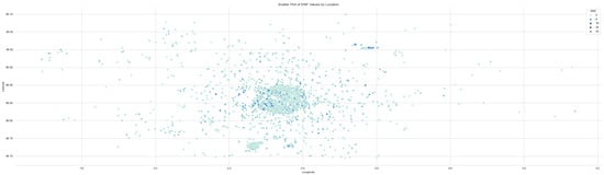
Figure 1.
The distributions of measurement points.
To prepare the data for analysis, we used a variety of scikit-learn library [24]. This library offered flexibility and powerful tools to present the results effectively. Our final dataset contains eight key variables:
- ID: This unique identifier helps track each antenna location.
- EMF (V/m): This variable represents the total electromagnetic field strength (summed across all bands) measured at each antenna.
- Urbanization degree: This variable, coded with 8 values based on [25], indicates the level of urbanization in a specific area.
- Population (expressed as the number of people per 100 m × 100 m): This variable, extracted from a population density dataset [26], represents the number of people living within a 100 m × 100 m square around each antenna.
- Built-up volume (m3): Derived from a spatial dataset [27], this variable indicates the total volume of buildings in the area surrounding each antenna.
- Built-up surface (m2): This variable, extracted from a dataset [28], represents the total surface area of buildings in the area, including residential and non-residential uses.
- Building height (m): This variable, derived from a building height dataset [29], indicates the average building height in the vicinity of each antenna.
- Settlement characteristics: This variable, based on the GHS-BUILT-C dataset [30], describes the inner structure and functionality of the built environment around each antenna.
2.2. Preprocessing Data
Standardization and Sampling
To improve the effectiveness of our machine learning models, we standardized the data using the z-score method. This technique ensures that all variables are on an equal footing for models to learn from. In essence, the z-score method subtracts the average value (mean) from each data point and then divides it by the standard deviation. This results in a new dataset where each variable has a mean of zero and a standard deviation of one. Crucially, we performed this standardization process separately for each training dataset that we used. This guaranteed that the models were trained and evaluated using data that were consistently scaled.
Before diving into model training, we took steps to ensure our data were clean and ready to use (Figure 2). First, we shuffled the initial dataset to prevent feature clustering and ensure a representative sampling of all possible conditions. For the model selection process, we utilized a combination of two methodologies to evaluate our machine learning algorithms: the shuffling method and 5-fold cross-validation. Initially, we randomized the order of entries within the model selection dataset, then split the data into training and validation pairs using a 70–30% split ratio. Next, we divided the training dataset into five subsets, applying the 5-fold cross-validation method. Standardization, as described in Figure 2, was performed for each split during the 5-fold cross-validation. This entire process was repeated 10 times. By integrating these methodologies, we generated 50 pairs of training and validation sets, enabling a robust evaluation of various interpolation methods. The shuffling method introduced variability and randomness into the selection process, while the 5-fold cross-validation ensured comprehensive coverage of the dataset in a systematic manner.
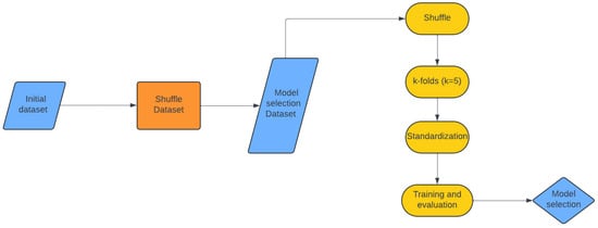
Figure 2.
The methodology’s flowchart.
2.3. Machine Learning Algorithms
The issue we need to tackle involves forecasting the electromagnetic radiation levels in outdoor environments, including urban, semi-urban, and rural areas, each with distinct topographical characteristics. To address this, we will use machine learning techniques. Machine learning is an umbrella term for a set of data analysis methods that can automate the development of models. It is a branch of artificial intelligence based on the idea that systems can be trained using a dataset to identify patterns and make decisions with minimal human intervention.
2.3.1. k-NN
The k-NN algorithm stands out as one of the most straightforward machine learning approaches. When applied to classification tasks, it determines the category by considering the majority category among the k-nearest neighbors. In regression problems, it estimates the value using a weighted mean function, represented by the formula , where denotes the estimated value. Alternatively, more advanced functions can be employed, such as weighting by the inverse of distances, as follows:
or using more mathematically complex distance functions, such as exponential weighting by distance or employing a Gaussian function (Gaussian kernel). Additionally, within the k-NN algorithm, we have the flexibility to change the distance function. A common approach involves exploring various values for the Minkowski distance (Equation (2)), as follows:
which allows for adapting the distance metric to better suit the characteristics of the dataset. In this study, we set the number of neighbors (k) to be the set , determining the quantity of nearest neighbors considered for predictions. Additionally, we adjusted two hyperparameters to enhance model performance. Firstly, for the distance function, we utilized the Minkowski distance with . Secondly, for the weight function, we adopted two different approaches—the first was to assign equal weight to all points within each neighborhood and the second was to use the weighted by the inverse of their distance.
2.3.2. Neural Networks
We will introduce the mathematical construct known as neural networks. These structures have garnered significant attention in recent times and have emerged as a fundamental concept in contemporary machine learning. However, their origins trace back to the inspiration drawn from the functioning of the human brain. Indeed, the inception of the first neural network can be attributed to the work by McCulloch and Pitts, who sought to model a biological neuron. A McCulloch and Pitts neuron is a function with
where denotes real numbers, d denotes a natural number, and denotes the real function with for and for . In terms of the neural network framework, the function denotes the activation function, denotes the threshold, and denotes weights. A more sophisticated model is the multilayer perceptron, which is the fundamental construction. In this research, we will use the [“Theory of Deep Learning” by Cambridge University Press]. A fully connected feedforward network is given by its architecture , where , and ; denotes the activation function, L denotes the number of layers, and with , denote the number of neurons in the input, output, and the l-th hidden layer, respectively. Let denote the number of parameters. Then, we can define the corresponding realization function , where each input and parameter set , consisting of . This means that for every l, is a real matrix and is a vector, where and
and is applied component-wise. Also, we refer to the matrices as the weighted matrices and to the vectors as the bias vectors. Additionally, we refer to and as activations and pre-activation functions of the neurons in the l-th layer. The width and the depth of the neural networks are defined as and L, respectively. In this study, we fine-tuned four hyperparameters to optimize model performance. Specifically, the hidden layers were tested with values of . The learning rate varied within the range of . The next hyperparameter, the solver, could either be ‘lbfgs’ (stochastic gradient descent) or ‘adam’ (another stochastic gradient-based optimizer). Additionally, we experimented with different activation functions, including ‘relu’, ‘identity’, and ‘logistic’.
2.3.3. Decision Trees (DTs)
Decision trees embody a non-parametric supervised learning approach suitable for both classification and regression assignments. A decision tree is a predictor , functioning as a mapping from the space of features to the discrete space . The most common situation is for to be binary. Usually, the splitting is based on one of the features of x or a predefined set of splitting rules. Their purpose is to build a model capable of forecasting the value of a target variable by deriving simple decision rules from the dataset’s features. Essentially, a tree functions as a piecewise constant estimation. Decision trees include several hyperparameters that can be tuned to control the model’s behavior and effectiveness. In this study, we focused solely on the depth as a hyperparameter, which was assigned values from the list .
2.4. Accuracy Criteria
There are numerous potential numerical calculations associated with modeling sample errors; the most commonly used is the mean square error (MSE). Ideally, this value should be zero. The mean square error as a criterion involves squaring the differences before calculating the mean, ensuring that all contributions are positive, and assigning a higher penalty to larger errors. This approach may better align with user concerns. In addition, we will use the root mean square error (RMSE), which is derived by taking the square root of the MSE, allowing the error metric to be expressed in the same units as the original data. In our error calculations, we will utilize both MSE and RMSE.
The root mean square error is the square root of the mean square error, which provides a measure of the average prediction error in the same units as the data we are trying to predict. The formula is as follows:
RMSE as an error index provides an interpretable measure of prediction accuracy, penalizes large errors, and aligns with the objectives of minimizing prediction deviations. These characteristics make it a robust choice for evaluating and comparing our regression models.
2.5. Heatmaps
A heatmap generated by machine learning regression algorithms shows how a predicted value changes in a specific area. Different colors represent different levels of the value, with warmer colors indicating higher levels. The machine learning model is taught to predict this value based on other information, and the heatmap visualizes the model’s predictions for different points. To create a heatmap using machine learning regression, the process (see Figure 3) starts with data collection, which involves gathering data that include input features (the set of variables as described in Section 2.1) and the target variable (electric field strength) for various points. The next step is model training, where a regression model (such as linear regression, random forest, support vector regression, or neural networks) is trained using the collected data to learn the relationship between the input features and the target variable. Once the model is trained, it is applied to make predictions across a grid or spatial area, generating predicted values for a dense set of locations or feature combinations, even in places where original data were not available. These predicted values are then visualized on a heatmap, where different colors represent varying ranges of predicted values, such as red for high values and blue for low values, creating a gradient effect. Regression-based machine learning heatmaps show predictive values rather than actual measurements, which makes them useful for forecasting in unsampled areas.
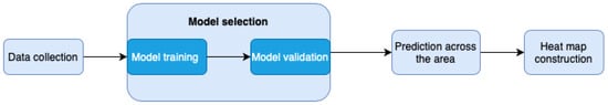
Figure 3.
The methodology of heatmap construction.
2.6. SHapley Additive exPlanations
The more complex the design of a machine learning model, the harder it is to understand. Deep learning is a prime example, where neural networks involve complex math that can be challenging for non-experts to grasp. As artificial intelligence and machine learning are used more and more in various applications, the need to explain how these models work has become increasingly important. This has led to the development of new techniques such as LIME [31] and SHAP [32], which bring explainability in machine learning to the field. To understand the new framework, let us first clarify what we mean by ‘model’ in this framework.
A set is called linearly separable if there exists a hyperplane H such that H can separate the set X into two subsets A and B. More formally, for any two points in X, if belongs to subset A and belongs to subset B, then H can be represented as a linear function as follows:
where w is called the weight vector. If , then x belongs to subset A, otherwise, it belongs to subset B. Imagine we have data to sort into two categories, like categories A and B. A common approach is to represent these data on a dimensional surface, like a plane. Each data point represents a dot, and its color would show its category.
Now, we can introduce the idea of a model. In this context, a model is like a dividing line on this plane that separates the dots in category A from those in category B. Mathematically, this line can be represented by the following:
Imagine all the possible dividing lines that we could draw on the plane to separate the data. These lines together form a category that we can call “models”. Our goal is to find the optimal dividing line among them, following certain rules, often minimizing some kind of error.
Now, let us introduce a new idea in machine learning: the “explanation model”. Based on SHAP [32], it is another model itself, but simpler and easier to understand than the original complex one.
We can think of it like this: sometimes it is easier to analyze a problem using a simpler version. Similarly, we can transform the original data x (such as lowering the resolution of an image) into a simpler format using a transformation while keeping the important details for the task.
Once we have these simplified data, we can use the explanation model to understand how the original model works. This explanation model is typically simpler, making it easier to understand how the model arrives at its decisions. Our framework uses a specific type of explanation model that relies on adding up the contributions of additive feature attribution methods, which have an explanation model that is a linear function:
where denotes binary variables, n denotes the number of simplified input features, and denotes the attribute effect. In the framework of SHAP, the main aim is to understand the impact of each feature on the model’s output. This involves assessing how the output of the model changes as we vary the input features. The mathematical background of this method has its origins in game theory, more specifically, Shapley regression values, which express the importance of each feature for linear models. This method calculates each attribute’s effect as follows:
where denotes the model over the subset of the feature set F. All these methods, which belong to additive feature attribution methods, share the following properties:
- Local accuracy: When the transformation is identified with x, then the explanation model matches the original model, i.e., .
- Missingness: Simply, if , then . This means that this feature has no attributable impact when . Missingness implies that a missing feature receives an attribution of zero.
- Consistency: The values remain constant unless there is a change in the contribution of a feature. More importantly, the consistency property says that if a feature becomes more important in making predictions, its Shapley value should also go up or stay the same.
3. Results
3.1. Descriptive Statistical Analysis
Table 1 indicates that the variable EMF shows an average of 1.52 V/m and a standard deviation of 1.74 V/m, reflecting significant variability in exposure levels between locations. The EMF values range from a minimum of 0.00 V/m to a maximum of 39.92 V/m, suggesting that although most areas experience low EMF, some locations have much higher levels. This indicates that the majority of radiation levels are relatively low and well within the safe range of 28 to 61 V/m, as suggested by the International Commission for Non-Ionizing Radiation Protection (ICNIRP). Even the maximum recorded value of 39.9 V/m does not exceed the recommended maximum level. POP statistics show that on average, 174 people reside within a 10 km2 area around the antenna, with a standard deviation of 144 people. The maximum number of people living in this area is 825. At first glance, an average of 17 people per km2 around each antenna seems more than satisfactory. However, considering that Paris spans an area of 105.4 km2, it is inevitable that the areas around each antenna would overlap. Therefore, we need to examine the distribution of the antennas on the map before reaching a final conclusion. V statistics indicate that the areas around the antennas are, on average, quite densely built-up, with a mean volume of 58.445 km3 and a standard deviation of 32.177 km3. The most densely built area has a volume of 306.729 km3. H statistics show that the buildings around the antennas have an average height of 5.8 m, with a standard deviation of 3.2 m. The maximum height recorded in the building is 30.6 m. S statistics reveal that the total surface area built up around the antennas is, on average, 38.12 m2, with a standard deviation of 26.47 m2. The largest built-up surface area is 100 m2. We can deduce that the areas studied are not heavily built up.

Table 1.
Measures of central tendency and dispersion of the dataset’s variables.
Figure 4 is the bar chart, which illustrates the frequencies of different categories of SMOD. The “Urban Centre” category dominates the chart with a significantly higher count compared to the other categories.
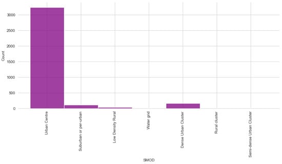
Figure 4.
SMOD distribution.
In Figure 5, we can observe two different aspects: first, the electromagnetic field strength distribution, and second, the distribution of electromagnetic field strength values at various points.
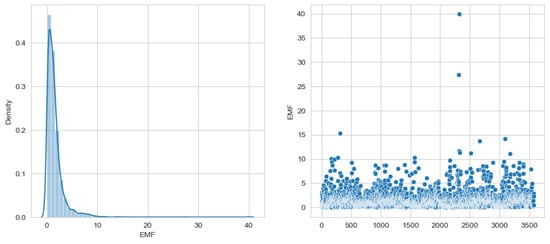
Figure 5.
EMF distribution.
Figure 6 offers a comprehensive visualization of the relationships between different variables in our dataset. It combines both histogram and scatter plots, providing a unique overview of the distributions and correlations of the dataset. The diagonal of the pair plot shows the histograms for each variable, which provides information on their distributions. The electromagnetic field (EMF) strength distribution is heavily skewed toward lower values, while the population (POP) shows a more spread-out distribution. The variable V (volume) displays a distribution concentrated around lower values but with a significant spread, indicating variability in the built-up volume around the antennas. The height (H) and surface (S) also show varied distributions, with some concentrations at lower values and notable spreads. Figure 6 illustrates the pairwise relationships between variables. There seems to be a strong positive correlation between V and H, suggesting that higher building volume values are associated with higher building heights. There appears to be no significant correlation between EMF and the other variables. Also, the EMF and POP plots suggest that population density alone does not directly predict EMF levels.
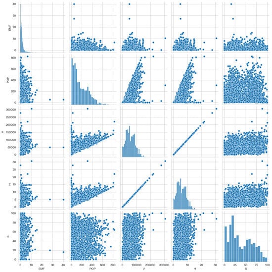
Figure 6.
Scatterplot of the dataset variables.
3.2. Machine Learning Analysis
The neural networks did not exhibit strong performance, with most configurations yielding suboptimal results (Table 2). However, a specific combination of hyperparameters stood out. The best result was achieved using five hidden layers, a learning rate of 0.01, and the logistic activation function, resulting in a root mean square error (RMSE) of 1.72 and a standard deviation of 0.77. This suggests that under carefully tuned conditions, neural networks have the potential for reasonable accuracy, although other configurations significantly underperformed.
Table 2.
The results of the optimal models.
In comparison, decision trees ranked second in terms of predictive accuracy, achieving an RMSE of 1.74 with a standard deviation of 0.20. The relatively low standard deviation indicates stable performance across different data subsets, suggesting that decision trees offer a consistent, albeit slightly less accurate, alternative to neural networks.
However, the k-nearest neighbors (kNN) algorithm outperformed both neural networks and decision trees, delivering the best overall results. Specifically, when using and (corresponding to the Euclidean distance), the model achieved an RMSE of 1.63 and a standard deviation of 0.20. This combination not only produced the lowest error but also showed excellent stability, with consistent results across different trials.
Further analysis of the RMSE distribution confirms that kNN exhibited the most stable performance. Even with a different configuration, such as , the algorithm managed an RMSE of 1.78 and a standard deviation of 0.21, which are still comparable to the best performance achieved by decision trees. This indicates that kNN is less sensitive to changes in hyperparameters than the other models, maintaining competitive accuracy under various settings.
The findings clearly demonstrate that kNN offers the best overall performance in terms of both error reduction and stability when compared to neural networks and decision trees. This robustness makes kNN a more reliable choice for this particular application, as it consistently delivers lower prediction errors. Figure 7, Figure 8, Figure 9 and Figure 10 provide visual summaries of these findings, illustrating the relative performances of the different algorithms in various hyperparameter configurations.
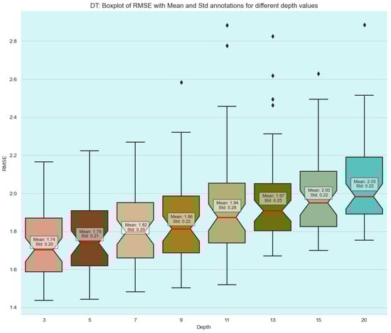
Figure 7.
Boxplots of decision tree model performances.
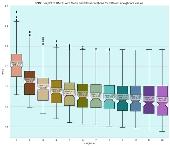
Figure 8.
Boxplots of k-NN model performances across different neighbors.
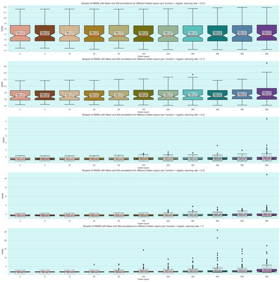
Figure 9.
Boxplots of neural network model performances across different logistic hyperparameters.
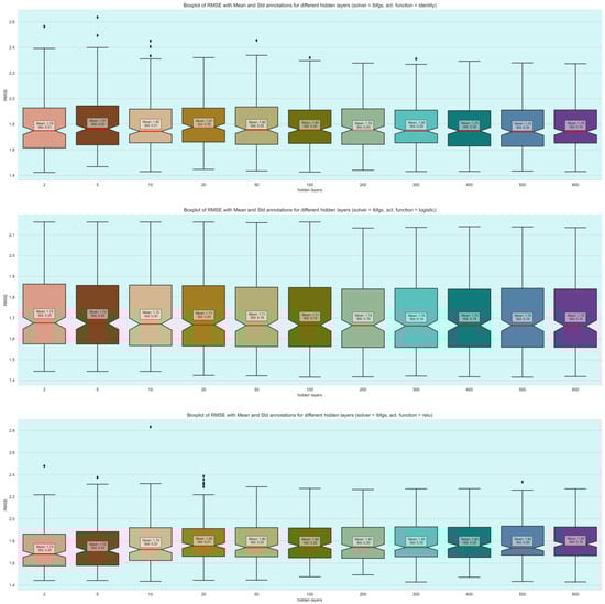
Figure 10.
Boxplots of neural network model performances across different hidden layers.
3.3. Electric Field Strength Prediction Map
The first image (Figure 11) shows a map with numerous red dots, representing the locations of electromagnetic field (EMF) measurements scattered throughout the urban area in the center of Paris. The map provides a clear view of each data point’s location but does not convey the intensity or concentration of values between these points. Therefore, it is necessary to refer to the second image, which is an overlay of the electric field strength map on the same urban area. This map uses different colors (yellow, green, and purple) to represent the intensity or density of the variable throughout the region. Areas with warmer colors, such as yellow or red, indicate higher values, while areas with cooler colors, such as green or purple, indicate lower values. This heatmap was generated using the optimal model, k-nearest neighbors (k-NN) with and , as the interpolation method (Figure 12).
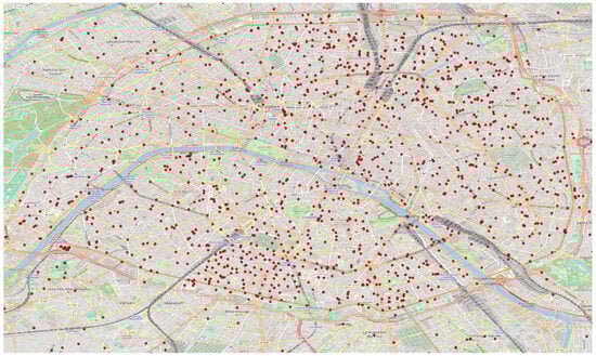
Figure 11.
The points of the measurements.
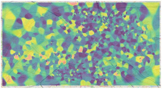
Figure 12.
The electric field strength prediction map.
3.4. Explainable Machine Learning
Figure 13 and Figure 14 display the mean absolute SHAP value for each feature, indicating the average impact on the model’s output magnitude. The features are ranked in descending order of importance. The feature representing the total volume of buildings in the area surrounding each antenna (V) has the highest mean SHAP value, suggesting it has the most significant impact on the model’s predictions. The population density feature (POP) is the second most important, but its impact is considerably lower than V. The total surface area of the buildings in the area (S) has a moderate impact on the model. The remaining features, including longitude, C, latitude, H, and SMOD, have minimal impact on the model’s output, as indicated by their low mean SHAP values.
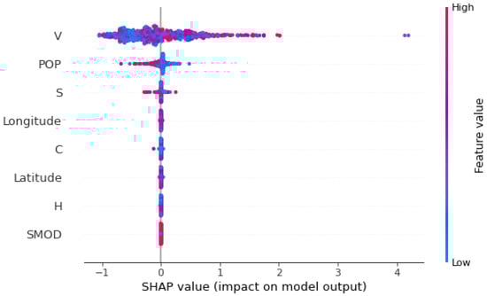
Figure 13.
Summary plot of SHapley Additive exPlanations (SHAP).
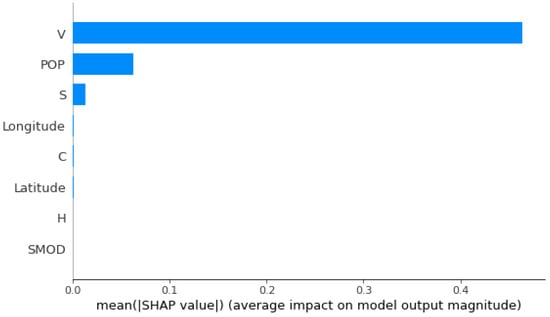
Figure 14.
Mean SHapley Additive exPlanations (SHAP) value plot.
From these SHAP plots, we have observed that the feature representing the total volume of buildings in the area surrounding each antenna (V) is the most critical in predicting the strength of the electromagnetic field in the kNN regression model. It consistently shows a high impact on the predictions. The characteristic population density (POP) also has a notable influence, although it is less pronounced than V. Other features like S, longitude, C, latitude, H, and SMOD have minimal impact on the model’s predictions.
4. Conclusions
The extensive evaluation of 410 machine learning models, which includes k-nearest neighbors (kNN), neural networks, and decision trees, established that the kNN algorithm is the most effective in predicting the strength of the electromagnetic field (EMF) in urban settings, especially when using geographic features as predictive variables. The kNN model consistently delivered the most reliable performance, achieving a root mean square error (RMSE) of 1.63 with a standard deviation of 0.20, thus surpassing both neural networks and decision trees in terms of predictive accuracy and stability. The superior performance of the kNN model can be attributed to its ability to exploit a comprehensive dataset that integrates not only EMF measurements but also various geographical and urban characteristics, including population density, levels of urbanization, and specific building attributes.
To gain a deeper understanding of the model’s predictive behavior, SHAP (SHapley Additive exPlanations) was employed as a key explainable machine learning technique. This approach provided valuable information on the factors driving the model predictions, revealing that the most influential characteristic was the total volume of buildings in the vicinity of each antenna. This characteristic consistently exhibited a significant impact on all predictions, underscoring its critical role in the decision-making process of the model. Population density emerged as another important factor, although its influence was less pronounced than that of building volume. Other features, such as the total surface area of buildings, contributed moderately to the predictions, whereas geographic coordinates like longitude and latitude were found to have minimal impact on the model’s outcomes.
Our research significantly advances the field of environmental monitoring by constructing highly accurate and dynamic maps of electromagnetic field strength using state-of-the-art machine learning techniques. The integration of a comprehensive dataset and explainable AI methods has enabled the identification of key factors that affect the strength of the EMF, leading to the development of robust and reliable predictive models. These EMF maps provide valuable information for policymakers, urban planners, and researchers, facilitating data-driven decision-making regarding public health, infrastructure development, and urban management. The findings of this study demonstrate the transformative potential of machine learning in the handling of complex environmental challenges, paving the way for more informed approaches to monitoring and managing electromagnetic exposure in urban environments. The creation of electromagnetic radiation level maps will contribute to various fields, including the following: (a) Risk assessment: These maps will facilitate the evaluation of environmental risks by identifying areas with elevated electromagnetic radiation levels. This information is essential for formulating risk management strategies and implementing preventive measures to protect public health and the environment. (b) Developing best practices: The maps will provide valuable data and insights that can be used to evaluate and optimize radiation protection protocols for the general population exposed to electromagnetic radiation. A subsequent step in the investigation involves not only broadening the comparative analysis to a wider range of cities but also improving the dataset with additional geographic variables. A more ambitious aim would be to incorporate temporal parameters to facilitate the development of real-time maps.
Author Contributions
Conceptualization, Y.K.; methodology, Y.K. and K.V.; software, I.P., I.K. and S.Z.; validation, Y.K. and I.P.; formal analysis, Y.K. and I.T.; investigation, Y.K., K.V. and I.T.; data curation, Y.K., I.P., K.V., S.Z. and I.K.; writing—original draft preparation, Y.K. and I.P.; writing—review and editing, Y.K., T.P., and I.T.; visualization, I.P.; supervision, Y.K., T.P. and I.F.; project administration, Y.K., T.P. and I.F. All authors have read and agreed to the published version of the manuscript.
Funding
This research received no external funding.
Institutional Review Board Statement
Not applicable.
Data Availability Statement
Data is contained within the article.
Conflicts of Interest
The authors declare no conflicts of interest.
Abbreviations
The following abbreviations are used in this manuscript:
| MDPI | Multidisciplinary Digital Publishing Institute |
| DOAJ | Directory of Open Access Journals |
| TLA | three-letter acronym |
| LD | linear dichroism |
References
- Cordelli, E.; Ardoino, L.; Benassi, B.; Consales, C.; Eleuteri, P.; Marino, C.; Sciortino, M.; Villani, P.; Brinkworth, M.H.; Chen, G.; et al. Effects of Radiofrequency Electromagnetic Field (RF-EMF) exposure on pregnancy and birth outcomes: A systematic review of experimental studies on non-human mammals. Environ. Int. 2023, 180, 108178. [Google Scholar] [CrossRef] [PubMed]
- Hansson Mild, K.; Mattsson, M.O.; Jeschke, P.; Israel, M.; Ivanova, M.; Shalamanova, T. Occupational Exposure to Electromagnetic Fields—Different from General Public Exposure and Laboratory Studies. Int. J. Environ. Res. Public Health 2023, 20, 6552. [Google Scholar] [CrossRef] [PubMed]
- Committee on Man and Radiation (COMAR). COMAR Technical Information Statement: Expert Reviews on Potential Health Effects of Radiofrequency Electromagnetic Fields and Comments on the BioInitiative Report. Health Phys. 2009, 97, 348–356. [Google Scholar] [CrossRef] [PubMed]
- Kashani, Z.A.; Pakzad, R.; Fakari, F.R.; Haghparast, M.S.; Abdi, F.; Kiani, Z.; Talebi, A.; Haghgoo, S.M. Electromagnetic fields exposure on fetal and childhood abnormalities: Systematic review and meta-analysis. Open Med. 2023, 18, 20230697. [Google Scholar] [CrossRef]
- Bosch-Capblanch, X.; Esu, E.; Dongus, S.; Oringanje, C.M.; Jalilian, H.; Eyers, J.; Oftedal, G.; Meremikwu, M.; Röösli, M. The effects of radiofrequency electromagnetic fields exposure on human self-reported symptoms: A protocol for a systematic review of human experimental studies. Environ. Int. 2022, 158, 106953. [Google Scholar] [CrossRef]
- Martin, S.; De Giudici, P.; Genier, J.C.; Cassagne, E.; Doré, J.F.; Ducimetière, P.; Evrard, A.S.; Letertre, T.; Ségala, C. Health disturbances and exposure to radiofrequency electromagnetic fields from mobile-phone base stations in French urban areas. Environ. Res. 2021, 193, 110583. [Google Scholar] [CrossRef]
- Ramirez-Vazquez, R.; Escobar, I.; Vandenbosch, G.A.; Arribas, E. Personal exposure to radiofrequency electromagnetic fields: A comparative analysis of international, national, and regional guidelines. Environ. Res. 2024, 246, 118124. [Google Scholar] [CrossRef]
- Aerts, S.; Deprez, K.; Verloock, L.; Olsen, R.G.; Martens, L.; Tran, P.; Joseph, W. RF-EMF Exposure near 5G NR Small Cells. Sensors 2023, 23, 3145. [Google Scholar] [CrossRef]
- Liu, S.; Tobita, K.; Onishi, T.; Taki, M.; Watanabe, S. Electromagnetic field exposure monitoring of commercial 28-GHz band 5G base stations in Tokyo, Japan. Bioelectromagnetics 2024, 45, 281–292. [Google Scholar] [CrossRef] [PubMed]
- Ramirez-Vazquez, R.; Escobar, I.; Vandenbosch, G.A.; Vargas, F.; Caceres-Monllor, D.A.; Arribas, E. Measurement studies of personal exposure to radiofrequency electromagnetic fields: A systematic review. Environ. Res. 2023, 218, 114979. [Google Scholar] [CrossRef]
- Carlos Estrada-Jiménez, J.; Pardo, E.; Roth, U.; Selmane, L.; Faye, S. Under the Hood of Electromagnetic Field Estimation and Evaluation in 5G Networks. IEEE Access 2024, 12, 88357–88369. [Google Scholar] [CrossRef]
- Jiang, T.; Skrivervik, A.K. The electromagnetic field exposure assessment based on Monte Carlo method for 5G base station in urban area. Chin. J. Radio Sci. 2023, 38, 903–910. [Google Scholar] [CrossRef]
- Iyare, R.N.; Volskiy, V.; Vandenbosch, G.A. Study of the electromagnetic exposure from mobile phones in a city like environment: The case study of Leuven, Belgium. Environ. Res. 2019, 175, 402–413. [Google Scholar] [CrossRef] [PubMed]
- Bhatt, C.R.; Henderson, S.; Sanagou, M.; Brzozek, C.; Thielens, A.; Benke, G.; Loughran, S. Micro-environmental personal radio-frequency electromagnetic field exposures in Melbourne: A longitudinal trend analysis. Environ. Res. 2024, 251, 118629. [Google Scholar] [CrossRef] [PubMed]
- Kiouvrekis, Y.; Manios, G.; Tsitsia, V.; Gourzoulidis, G.; Kappas, C. A statistical analysis for RF-EMF exposure levels in sensitive land use: A novel study in Greek primary and secondary education schools. Environ. Res. 2020, 191, 109940. [Google Scholar] [CrossRef]
- Panagiotakopoulos, T.; Kiouvrekis, Y.; Misthos, L.M.; Kappas, C. RF-EMF Exposure Assessments in Greek Schools to Support Ubiquitous IoT-Based Monitoring in Smart Cities. IEEE Access 2023, 11, 7145–7156. [Google Scholar] [CrossRef]
- Ibrani, M.; Maloku, H.; Kastrati, A.; Mustafa, K. In-Situ Measurement of 5G Electromagnetic Exposure Levels in Urban Environments. In Proceedings of the 2024 47th MIPRO ICT and Electronics Convention (MIPRO), Opatija, Croatia, 20–24 May 2024; pp. 822–825. [Google Scholar] [CrossRef]
- Wang, S.; Wiart, J. Sensor-Aided EMF Exposure Assessments in an Urban Environment Using Artificial Neural Networks. Int. J. Environ. Res. Public Health 2020, 17, 3052. [Google Scholar] [CrossRef]
- Wang, S.; Mazloum, T.; Wiart, J. Prediction of RF-EMF Exposure by Outdoor Drive Test Measurements. Telecom 2022, 3, 396–406. [Google Scholar] [CrossRef]
- Mallik, M.; Tesfay, A.A.; Allaert, B.; Kassi, R.; Egea-Lopez, E.; Molina-Garcia-Pardo, J.M.; Wiart, J.; Gaillot, D.P.; Clavier, L. Towards Outdoor Electromagnetic Field Exposure Mapping Generation Using Conditional GANs. Sensors 2022, 22, 9643. [Google Scholar] [CrossRef] [PubMed]
- Mazloum, T.; Wang, S.; Wiart, J. RF-EMF exposure induced by distributed antenna system in the subway station. In Proceedings of the 2022 3rd URSI Atlantic and Asia Pacific Radio Science Meeting (AT-AP-RASC), Gran Canaria, Spain, 29 May–3 June 2022; pp. 1–2. [Google Scholar] [CrossRef]
- Shi, D.; Li, W.; Cui, K.; Lian, C.; Liu, X.; Qi, Z.; Xu, H.; Zhou, J.; Liu, Z.; Zhang, H. Electromagnetic radiation estimation at the ground plane near fifth-generation base stations in China by using machine learning method. IET Microw. Antennas Propag. 2024, 18, 391–401. [Google Scholar] [CrossRef]
- Agence nationale des fréquences (ANFR). Frequency management and monitoring in France. Official Website. Available online: https://www.anfr.fr/accueil (accessed on 4 January 2025).
- Pedregosa, F.; Varoquaux, G.; Gramfort, A.; Michel, V.; Thirion, B.; Grisel, O.; Blondel, M.; Prettenhofer, P.; Weiss, R.; Dubourg, V.; et al. Scikit-learn: Machine Learning in Python. J. Mach. Learn. Res. 2011, 12, 2825–2830. Available online: https://scikit-learn.org (accessed on 4 January 2025).
- Schiavina, M.; Melchiorri, M.; Pesaresi, M. GHS-SMOD R2023A—GHS Settlement Layers, Application of the Degree of Urbanisation Methodology (Stage I) to GHS-POP R2023A and GHS-BUILT-S R2023A, Multitemporal (1975–2030); Technical Report; European Commission, Joint Research Centre (JRC): Brussels, Belgium, 2023. [Google Scholar] [CrossRef]
- Schiavina, M.; Freire, S.; Carioli, A.; MacManus, K. GHS-POP R2023A—GHS Population Grid Multitemporal (1975–2030); Technical Report; European Commission, Joint Research Centre (JRC): Brussels, Belgium, 2023. [Google Scholar] [CrossRef]
- Pesaresi, M.; Politis, P. GHS-BUILT-V R2023A—GHS Built-Up Volume Grids Derived from Joint Assessment of Sentinel2, Landsat, and Global DEM Data, Multitemporal (1975–2030); Technical Report; European Commission, Joint Research Centre (JRC): Brussels, Belgium, 2023. [Google Scholar] [CrossRef]
- Pesaresi, M.; Politis, P. GHS-BUILT-S R2023A—GHS Built-Up Surface Grid, Derived from Sentinel2 Composite and Landsat, Multitemporal (1975–2030); Technical Report; European Commission, Joint Research Centre (JRC): Brussels, Belgium, 2023. [Google Scholar] [CrossRef]
- Pesaresi, M.; Politis, P. GHS-BUILT-H R2023A—GHS Building Height, Derived from AW3D30, SRTM30, and Sentinel2 Composite (2018); Technical Report; European Commission, Joint Research Centre (JRC): Brussels, Belgium, 2018. [Google Scholar] [CrossRef]
- Pesaresi, M.; Politis, P. GHS-BUILT-C R2023A—GHS Settlement Characteristics, Derived from Sentinel2 Composite (2018) and Other GHS R2023A Data; Technical Report; European Commission, Joint Research Centre (JRC): Brussels, Belgium, 2023. [Google Scholar] [CrossRef]
- Ribeiro, M.T.; Singh, S.; Guestrin, C. “Why Should I Trust You?”: Explaining the Predictions of Any Classifier. In Proceedings of the 22nd ACM SIGKDD International Conference on Knowledge Discovery and Data Mining, San Francisco, CA, USA, 13–17 August 2016; KDD’16. pp. 1135–1144. [Google Scholar] [CrossRef]
- Lundberg, S.M.; Lee, S.I. A unified approach to interpreting model predictions. In Proceedings of the 31st International Conference on Neural Information Processing Systems, Red Hook, NY, USA, 4–9 December 2017; NIPS’17. pp. 4768–4777. [Google Scholar]
Disclaimer/Publisher’s Note: The statements, opinions and data contained in all publications are solely those of the individual author(s) and contributor(s) and not of MDPI and/or the editor(s). MDPI and/or the editor(s) disclaim responsibility for any injury to people or property resulting from any ideas, methods, instructions or products referred to in the content. |
© 2025 by the authors. Licensee MDPI, Basel, Switzerland. This article is an open access article distributed under the terms and conditions of the Creative Commons Attribution (CC BY) license (https://creativecommons.org/licenses/by/4.0/).