Article

Modeling of Malware Propagation in Wireless Mobile Networks with Hotspots Considering the Movement of Mobile Clients Based on Cosine Similarity

1
Graduate School of Interdisciplinary Science and Engineering in Health Systems, Okayama University, Okayama 700-8530, Japan
2
Faculty of Science and Engineering, Doshisha University, Kyoto 610-0321, Japan
3
Faculty of Engineering Science, Kansai University, Osaka 564-8680, Japan
*
Author to whom correspondence should be addressed.
Electronics 2025, 14(17), 3528; https://doi.org/10.3390/electronics14173528
Submission received: 4 August 2025 / Revised: 27 August 2025 / Accepted: 2 September 2025 / Published: 4 September 2025

Abstract

In this paper, we propose a deterministic epidemic model for malware propagation in wireless mobile environments, taking into account the presence of hotspots. Conventional epidemic models for wireless mobile environments typically assume that mobile hosts randomly move in a given area. However, in real-world scenarios, hotspots such as restaurants and universities often attract large gatherings of people. Therefore, the assumption of purely random movement is not suitable for modeling these scenarios. To realistically represent the movement patterns of mobile hosts, we incorporate the influence of hotspots into our model. Specifically, we formulate a system of Ordinary Differential Equations (ODEs) that captures the infection dynamics in scenarios where one or more hotspots affect host mobility. Our model introduces non-uniform movement probabilities based on cosine similarity, allowing us to reflect the tendency of mobile hosts to cluster around specific locations. By applying these movement probabilities to the ODEs, our epidemic model provides a more accurate representation of malware spreading behavior in hotspot-affected environments. We investigate how malware propagates through mobile hosts and compare the dynamics between the conventional and our proposed models. Numerical experiments demonstrate that our epidemic model effectively captures malware spreading behavior in mobile scenarios with hotspots.

1. Introduction

In recent years, mobile devices such as smartphones, tablets, and IoT-enabled sensors have become indispensable in daily life [1]. With the widespread adoption of wireless communication technologies, users frequently connect to various networks in public spaces. As these technologies become more prevalent and interconnected, concerns about their security have intensified. In particular, malware targeting mobile environments has emerged as a significant threat. Such malware often propagates through wireless communication interfaces such as Bluetooth and Wi-Fi [2,3,4].
Consequently, the awareness of security issues has been increasing, and many approaches have been proposed to enhance security and reliability in communication systems, such as an intrusion detection-embedded chaotic encryption method [5]. Furthermore, to analyze and mitigate the risk of malware propagation, various epidemic models based on simulation or mathematical frameworks have been proposed, by drawing inspiration from human epidemic models such as the Susceptible–Infected–Recovered–Susceptible (SIRS) model [6]. As an epidemic model for analyzing the propagation dynamics of Bluetooth-based worms in smartphone environments, Gonzalez et al. [7] proposed a simulation-based spatio-temporal model that captures the movement behavior of mobile hosts. The application of such epidemic models offers an effective approach for mitigating malware infection threats. Although simulation-based models evaluate infection dynamics through simulation experiments, they often lack mathematical tractability. This limits theoretical insight and makes it difficult to generalize findings across different parameter settings. Therefore, we are motivated to develop a deterministic model that provides a structured basis for theoretical investigation. In particular, the SIRS epidemic model provides a suitable macroscopic framework, as it captures the aggregate, long-term dynamics of malware diffusion rather than the fine-grained behavior of a single malware instance.
As a preliminary step in this direction, in [8], we proposed a deterministic epidemic model that represents malware infection through mobile hosts in a wireless mobile environment within a given closed area based on the SIRS framework. This model is one of the mathematical frameworks used to analyze malware propagation. The epidemic model employs a system of Ordinary Differential Equations (ODEs) to analyze the behavior of malware propagation on mobile hosts. In this model, each mobile host randomly moves within the area, assuming uniform movement without directional preference. This assumption effectively captures the basic propagation patterns of malware in wireless mobile environments. Compared to simulation-based approaches, the ODE-based framework facilitates clearer insights into system dynamics and allows for systematic examination of the impact of model parameters on malware propagation.
However, in reality, mobile hosts tend to congregate around specific popular locations, known as hotspots, such as restaurants, cafes, train stations, and university campuses. In addition, previous empirical studies have shown that human and mobile device movements are far from uniform, exhibiting strong regularities and hotspot-oriented aggregation patterns [7,9]. Hotspots naturally attract higher densities of mobile hosts, thereby increasing the risk of rapid malware propagation. Consequently, modeling mobility using uniform transition probabilities fails to accurately reflect the actual movement behavior of mobile hosts. In particular, in urban environments, incorporating hotspot-aware directional bias into a mathematically tractable ODE-based model remains a significant challenge. To the best of our knowledge, no existing deterministic model has explicitly addressed this issue.
To address this issue, we propose a deterministic epidemic model that incorporates non-uniform mobility influenced by the presence of hotspots, which extends the concept introduced in our previous work [8]. Our proposed model introduces a system of ODEs that offers a mathematically grounded way to explore how directional movement bias influences infection dynamics. The epidemic model introduces location-dependent movement probabilities, calculated based on the cosine similarity [10,11,12] between a mobile host’s position vector and the directional vectors of nearby hotspots. Cosine similarity provides a measure of angular proximity between vectors, enabling a mathematically tractable method for prioritizing movement toward nearby hotspots. These weighted probabilities are then integrated into the system of ODEs to more realistically capture the dynamics of malware propagation. We investigate how malware propagates through mobile hosts and compare the resulting dynamics between the conventional and our proposed models. Numerical experiments demonstrate that our epidemic model effectively captures malware spreading behavior in mobile scenarios with hotspots.
The contributions of this paper are summarized as follows:
  • We propose a novel deterministic epidemic model that incorporates non-uniform mobility influenced by the presence of hotspots, addressing the limitations of existing models based on uniform movement assumptions.
  • We introduce a location-dependent mobility mechanism using cosine similarity to model the directional tendency of mobile hosts toward nearby hotspots in a mathematically tractable manner.
  • We formulate a system of ODEs that integrates the proposed mobility model to analyze the dynamics of malware propagation in hotspot-influenced environments.
  • Through numerical experiments, we demonstrate that the proposed model captures malware spreading behavior in mobile scenarios with hotspots.
The remainder of this paper is organized as follows. Section 2 reviews related work. Section 3 describes the system model. Section 4 formulates the proposed epidemic model incorporating hotspot-influenced mobility. Section 5 presents numerical experiments and comparative analyses. Section 6 discusses model implications, extensibility, and limitations. Finally, Section 7 concludes the paper and outlines directions for future work.

2. Related Work

2.1. Evolution of Cyber Attacks

With the recent advancements in machine learning, particularly deep learning [13], cyber attacks leveraging machine learning techniques have emerged [14,15]. As a notable example, Kudo et al. [16] introduced the concept of self-evolving botnets, which utilize distributed machine learning to autonomously discover host vulnerabilities by exploiting the computational resources of infected zombie devices. Simulation experiments based on a continuous-time Markov chain demonstrated the high infectivity of these botnets. Shi et al. [17] presented a method for spoofing wireless signals using Generative Adversarial Networks (GANs), which are trained to mimic user behavior within target networks. Additionally, Li et al. [18,19] developed evasion techniques based on GANs to circumvent traditional malware detection systems.
In addition to machine learning-based threats, several real-world vulnerabilities in wireless communication protocols have raised significant security concerns. Lonzetta et al. [2] provided a comprehensive taxonomy of Bluetooth-related attacks and demonstrated that Bluetooth vulnerabilities can be exploited not only for data theft and device control but also for malware propagation. The paper introduced several Bluetooth-based worm attacks, including Cabir, Mabir, and Lasco, which exploit vulnerabilities in the pairing process and protocol stack to spread autonomously. These findings suggest that Bluetooth could serve as a potential vector for malware diffusion, particularly in IoT environments.
An example of such a vulnerability is BlueBorne [20,21], a flaw in Bluetooth protocol stacks that allows remote code execution when Bluetooth is enabled, even without any user interaction. This enables malware to propagate via Bluetooth without requiring user input. To further explore such vulnerabilities, Ruge et al. [22] proposed Frankenstein, a fuzzing framework specifically designed for analyzing Bluetooth firmware. Their framework effectively uncovered remote code execution (RCE) vulnerabilities that also required no user interaction. In particular, they demonstrated that the BlueFrag vulnerability, affecting Android 8 and 9, could be triggered via malformed L2CAP responses. These findings reinforce the notion that autonomous Bluetooth-based malware propagation is technically feasible, especially in short-range IoT communication scenarios.
Accordingly, given the evolution of malware toward more intelligent and autonomous behavior, it is increasingly important to analyze their propagation dynamics and develop effective countermeasures. Mathematical and computational modeling provides a powerful approach to understanding how malware spreads and to evaluating the impact of various parameters under diverse scenarios.

2.2. Epidemic Model

Epidemic models have been widely employed to analyze the dynamics of malware propagation in networked systems and are generally categorized into two main types: deterministic models and stochastic models.
Deterministic models represent the average behavior of systems using ODEs, following the classical framework of epidemiological models such as the SIRS model [6]. For example, Xiao et al. [23] proposed a Susceptible–Exposed–Infected–Quarantine–Recovered (SEIQR) model based on ODEs to represent worm propagation in mobile Internet environments. Similarly, Shen et al. [24] introduced a deterministic epidemic model for mobile wireless sensor networks that incorporates node mobility, enabling a more realistic analysis of malware spreading. These models are effective for capturing macroscopic infection trends but often rely on simplifying assumptions, such as homogeneous host mixing and uniform mobility.
In contrast, stochastic models account for random behavior in host movement and infection events. Okamura et al. [25] developed a continuous-time Markov chain-based SIS model and proposed the Kill Signal (KS) model to evaluate intervention mechanisms. Peng et al. [26] employed a semi-Markov process to simulate worm propagation on social graphs, while Gonzalez et al. [7] utilized cellular automata combined with compartment models to simulate Bluetooth worm diffusion. Although stochastic models can express randomness and discrete state transitions in a fine-grained manner, they often suffer from high computational cost and limited scalability, especially in large-scale network simulations. Moreover, because of their probabilistic nature, the results may vary across runs, making reproducibility and analytical tractability more challenging.
While stochastic models can flexibly incorporate non-uniform mobility by assigning probabilistic movement rules, deterministic models face greater challenges in explicitly formulating directional biases toward specific locations. In particular, to the best of our knowledge, no existing deterministic model has addressed how to represent user mobility in environments with identifiable hotspots, such as cafes, train stations, or university campuses.

2.3. Mobility Modeling and Cosine Similarity

In epidemic modeling, host mobility plays a crucial role in shaping diffusion dynamics, particularly in mobile and spatially structured environments. While stochastic models can flexibly incorporate non-uniform mobility by assigning probabilistic movement rules, deterministic models face greater challenges in explicitly formulating directional biases toward specific locations.
In modeling human mobility, both deterministic and stochastic approaches commonly represent movement patterns using location visit frequencies or probabilistic transition rules. To compare such patterns, cosine similarity has been widely used to quantify behavioral similarity between different users. For example, Fan et al. [11], Memon et al. [12], and Toole et al. [10] adopted cosine similarity to evaluate how similarly two users behave based on their historical location vectors. These approaches effectively capture the resemblance of mobility patterns across users. Peng et al. [27] proposed a movement-aware distance metric between trajectories by incorporating the cosine similarity of spatial direction vectors. Their method evaluates the angular consistency between movement paths and penalizes directional misalignment, thereby providing a foundation for representing movement tendencies toward specific destinations. However, such direction-based cosine metrics have not yet been incorporated into epidemic models for analyzing malware propagation.
In this paper, we propose a deterministic epidemic model that integrates directionally biased mobility toward hotspots using cosine similarity. The model is formulated as a system of ODEs and aims to enhance the accuracy of malware propagation analysis in urban mobile environments. By embedding cosine-based movement probabilities, the proposed model captures realistic user mobility patterns and extends existing modeling approaches to incorporate spatial directionality.

3. System Model

Our proposed epidemic model describes the dynamics of malware propagation using ODEs, following the same principles as traditional epidemic models for communicable diseases, such as the SIRS model [6]. Note that this paper adopts a macroscopic perspective, aiming to capture the aggregate infection dynamics of mobile hosts under the influence of hotspots. In contrast to microscopic models that track the detailed behavior of a single malware strain over a limited duration, our approach focuses on the long-term evolution of potential threats in the network. In this section, we first explain the standard SIRS model, followed by a detailed explanation of the system model.

3.1. Standard SIRS Model

We assume that there exist malware and H N hosts in a given area. Note that the standard SIRS model does not consider host mobility. In the SIRS model, each host in the area belongs to a Susceptible (S), Infected (I), or Recovered (R) state as shown in Figure 1. Hosts in state S are not currently infected but are vulnerable to infection. Hosts in state I are infected with malware. Hosts in state R are recovered and possess temporary protection against infection. The transitions between the states occur according to the following events:
  • Susceptible hosts become infected with the malware through contact with infected hosts and transition to state I.
  • Infected hosts eliminate the malware from themselves and then transition to state R.
  • Recovered hosts become susceptible again due to the discovery of a new vulnerability and transition to state S.
Let S ( t ) , I ( t ) , and R ( t ) denote the fraction of hosts belonging to the states S, I, and R, respectively, at time t ( t 0 ), where S ( t ) + I ( t ) + R ( t ) = H . The SIRS model represents the infection dynamics with the following ODEs:
d d t S ( t ) = α S ( t ) I ( t ) + γ R ( t ) ,
d d t I ( t ) = α S ( t ) I ( t ) β I ( t ) ,
d d t R ( t ) = β I ( t ) γ R ( t ) ,
where α , β , and γ represent the malware infection rate, malware elimination rate, and vulnerability discovery rate, respectively. In (1) and (2), the term α S ( t ) I ( t ) represents the average number of susceptible hosts getting infected per unit time at time t. In (2) and (3), the term β I ( t ) indicates the average number of infected hosts that eliminate the malware per unit time at time t. In (1) and (3), the term γ R ( t ) denotes the average number of recovered hosts that become susceptible again due to the discovery of new vulnerabilities per unit time at time t.
The standard SIRS model assumes a simplified scenario in which all hosts can interact with each other at any time t, without considering host mobility. It simply models the temporal evolution of the fraction of hosts in each state. By extending this SIRS framework, the proposed epidemic model incorporates hotspot-aware mobility into wireless mobile environments.

3.2. Mobility and State Transition Model

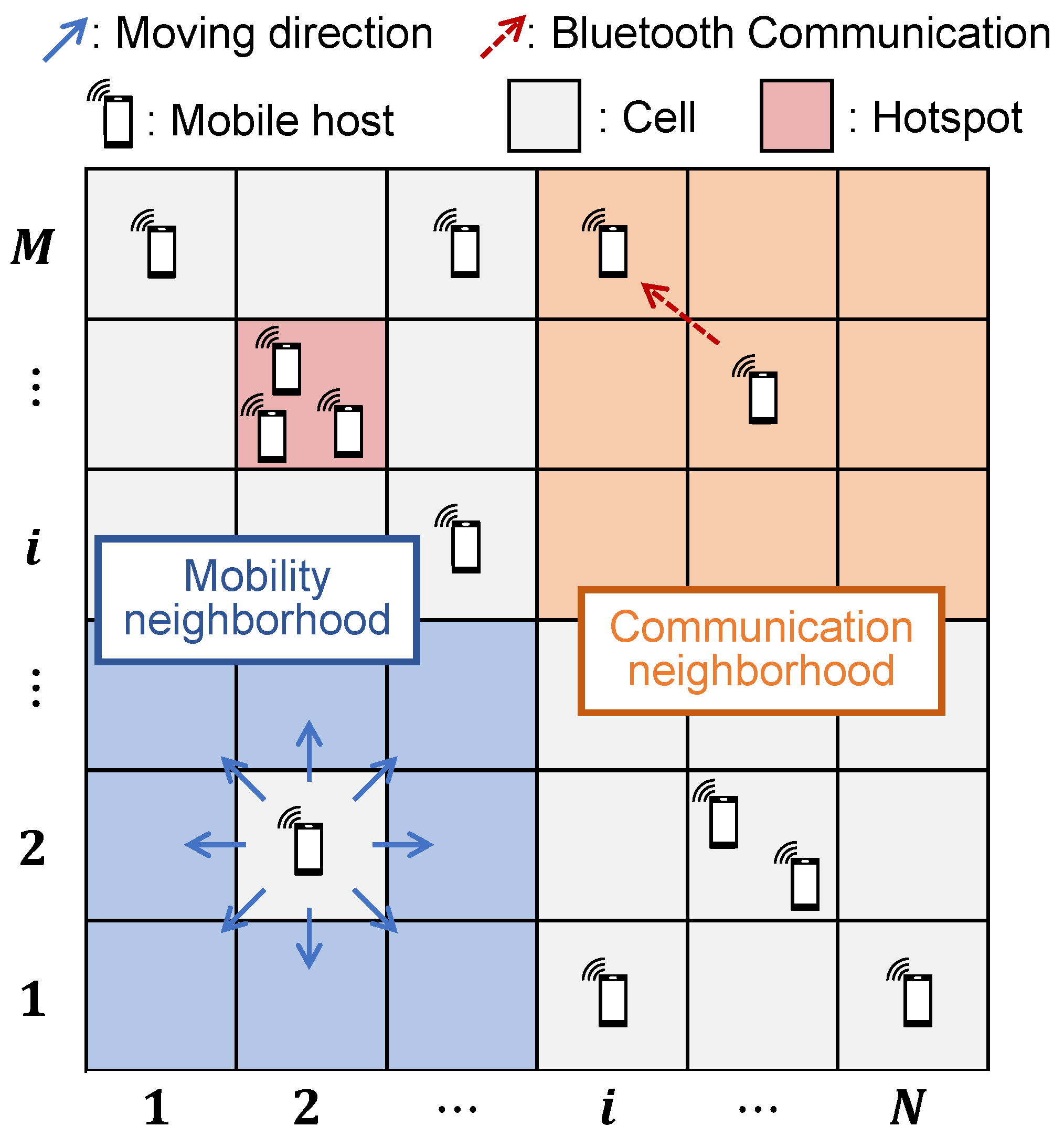
Figure 2 illustrates the system model assumed in this paper. We consider a closed area which is represented as a two-dimensional grid G consisting of M × N cells. For a given cell ( i , j ) G , the communication neighborhood denoted by C ( i , j ) ( 1 i M , 1 j N , i , j N ) is defined as follows:
C ( i , j ) = { ( m , n ) : | m i | 1 , | n j | 1 } ,
where the set C ( i , j ) corresponds to the orange-colored area (communication neighborhood) in Figure 2. Furthermore, the mobility neighborhood of cell ( i , j ) is defined as follows:
A ( i , j ) = C ( i , j ) { ( i , j ) } .
This corresponds to the adjacent cells of ( i , j ) excluding the cell itself, as indicated by the blue-colored area (mobility neighborhood) in Figure 2. We assume that some cells are selected as hotspots. In Figure 2, a hotspot is represented by a specific cell highlighted in red.
A finite set H of mobile hosts is distributed over this grid. Each host resides in one of the cells and is allowed to probabilistically move to one of the cells in the mobility neighborhood A ( i , j ) . Similarly, a host located at cell ( i , j ) can communicate with other hosts within its communication neighborhood C ( i , j ) . We define the position of a host h H at time t ( t 0 ) as c h ( t ) = ( i , j ) , where ( i , j ) denotes the cell in which the host resides. Here, ( i , j ) always denotes a cell index in the grid, so the host’s location is tracked only at the cell level, which serves as an approximation of its actual physical position. A mobile host located in cell ( i , j ) G can move to its next position by selecting one of the mobility neighborhood A ( i , j ) based on the movement strategy defined later. For example, if host h at cell ( i , j ) moves to the right at time t, then c h ( t ) = ( i , j + 1 ) , where we assume instantaneous movement between cells. State transitions of each host at cell ( i , j ) G occur according to the following rules:
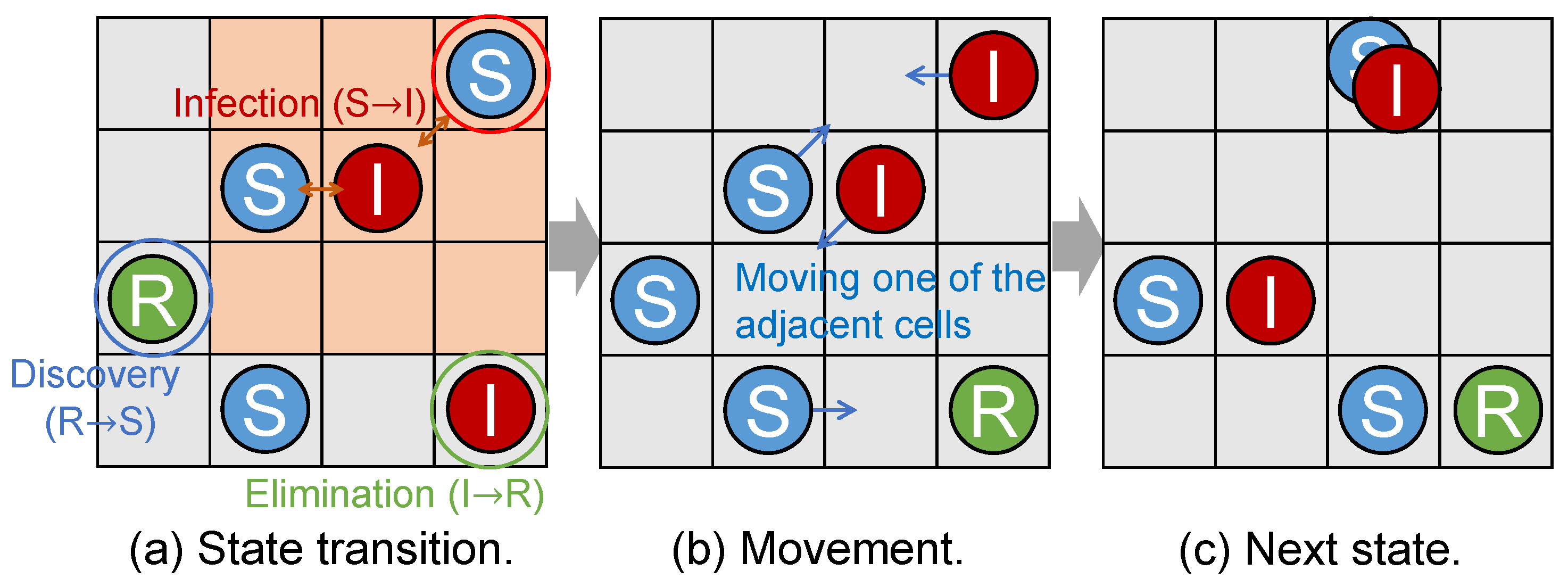
(1)
An infected host located at cell ( i , j ) G infects a susceptible host located in its neighborhood C ( i , j ) according to a Poisson process with the infection rate α . The susceptible host transitions to the infected state.
(2)
An infected host eliminates the malware according to a Poisson process with the elimination rate β . The infected host transitions to the recovered state.
(3)
A recovered host becomes susceptible again due to the discovery of a new vulnerability according to a Poisson process with the elimination rate γ . The recovered host transitions to the susceptible state.
(4)
A host located at cell ( i , j ) G moves to one of adjacent cells A ( i , j ) according to a Poisson process with the moving rate μ . The destination cell is selected based on movement strategies discussed later.
Figure 3 illustrates an example of state transition process. In this example, a susceptible host becomes infected by contact with an infected host in one of its neighboring cells. Additionally, an infected host eliminates the malware, and a recovered host becomes susceptible again due to the discovery of a new vulnerability (Figure 3a). These hosts then transition to the I, R, and S states, respectively (Figure 3b). Furthermore, some hosts move to one of their adjacent cells (Figure 3b,c).

4. Proposed Epidemic Model

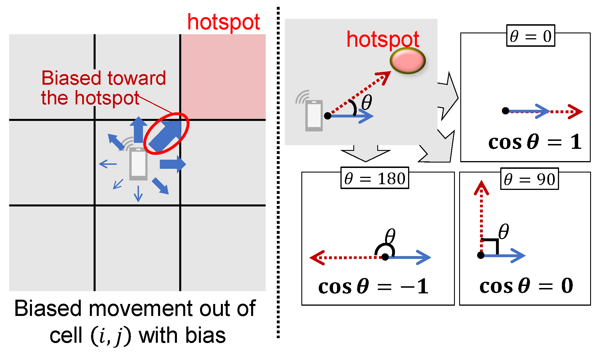
In the proposed model, mobile hosts tend to move in the direction of nearby hotspots as illustrated in Figure 4. As shown in the figure, the degree of movement bias depends on the angle between the host’s movement direction and the direction toward nearby hotspots. This directional preference is quantified using the cosine of the angle θ , where cos θ = 1 indicates the direction is exactly toward the hotspot, and cos θ = 1 indicates it is in the opposite direction. In particular, we employ cosine similarity to determine the directional preference, i.e., the movement probabilities to adjacent cells. As discussed in Section 2.3, cosine similarity has been used in human mobility models and can also be applied to malware propagation on mobile hosts.
In what follows, we first explain the deterministic epidemic model for mobile hosts. Then, we discuss the movement strategy of mobile hosts, which considers hotspots based on cosine similarity.

4.1. Epidemic Model of Malware Propagation on Mobile Hosts

We first describe the deterministic epidemic model on mobile hosts based on the model discussed in our previous work [8]. Let S ( i , j ) ( t ) , I ( i , j ) ( t ) , and R ( i , j ) ( t ) denote the number of susceptible, infected, and recovered hosts, respectively, in cell ( i , j ) at time t. Note that S ( t ) = ( i , j ) G S ( i , j ) ( t ) , I ( t ) = ( i , j ) G I ( i , j ) ( t ) , and R ( t ) = ( i , j ) G R ( i , j ) ( t ) hold. The epidemic model based on the SIRS model represents the infection dynamics with the following ODEs, where i = 1 , 2 , , M and j = 1 , 2 , , N :
d d t S ( i , j ) ( t ) = α S ( i , j ) ( t ) ( m , n ) C ( i , j ) I ( m , n ) ( t ) + γ R ( i , j ) ( t ) μ ( m , n ) A ( i , j ) P ( i , j ) ( m , n ) S ( i , j ) ( t ) + μ ( m , n ) A ( i , j ) P ( m , n ) ( i , j ) S ( m , n ) ( t ) ,
d d t I ( i , j ) ( t ) = α S ( i , j ) ( t ) ( m , n ) C ( i , j ) I ( m , n ) ( t ) β I ( i , j ) ( t ) μ ( m , n ) A ( i , j ) P ( i , j ) ( m , n ) I ( i , j ) ( t ) + μ ( m , n ) A ( i , j ) P ( m , n ) ( i , j ) I ( m , n ) ( t ) ,
d d t R ( i , j ) ( t ) = β I ( i , j ) ( t ) γ R ( i , j ) ( t ) μ ( m , n ) A ( i , j ) P ( i , j ) ( m , n ) R ( i , j ) ( t ) + μ ( m , n ) A ( i , j ) P ( m , n ) ( i , j ) R ( m , n ) ( t ) ,
where P ( i , j ) ( m , n ) represents the probability that a host moves from cell ( i , j ) to cell ( m , n ) . In (4) and (5), the term α S ( i , j ) ( t ) { ( m , n ) I ( m , n ) ( t ) } represents that the average number of susceptible hosts on cell ( i , j ) could become infected with the malware through contact with infected hosts located on neighborhood cells C ( i , j ) . In (5) and (6), the term β I ( i , j ) ( t ) represents that the average number of infected hosts on cell ( i , j ) that eliminate the malware. In (4) and (6), the term γ R ( i , j ) ( t ) represents the average number of recovered hosts that become susceptible again due to the discovery of new vulnerabilities.
All terms multiplied by μ represent host movement, where the positive terms indicate the average number of hosts migrating into cell ( i , j ) G from adjacent cells, while the negative terms indicate the average number of hosts migrating out of cell ( i , j ) to adjacent cells. The movement probability P ( i , j ) ( m , n )   ( ( m , n ) A ( i , j ) ) is determined based on the movement strategy.

4.2. Movement Strategy

In what follows, we discuss two movement strategies. One is the random movement strategy and the other is the hotspot-aware movement strategy introduced in the proposed method.

4.2.1. Random Movement Strategy

The simplest movement strategy is to move randomly [8], regardless of the presence of hotspots. In this strategy, the movement probability P ( i , j ) ( m , n ) ( ( m , n ) A ( i , j ) ) is defined as
P ( i , j ) ( m , n ) = 1 | A ( i , j ) | .
Specifically, this strategy assumes that mobile hosts move uniformly to all adjacent cells. Accordingly, the movement probability P ( i , j ) ( m , n ) is defined as the reciprocal of the number of adjacent cells in (7).
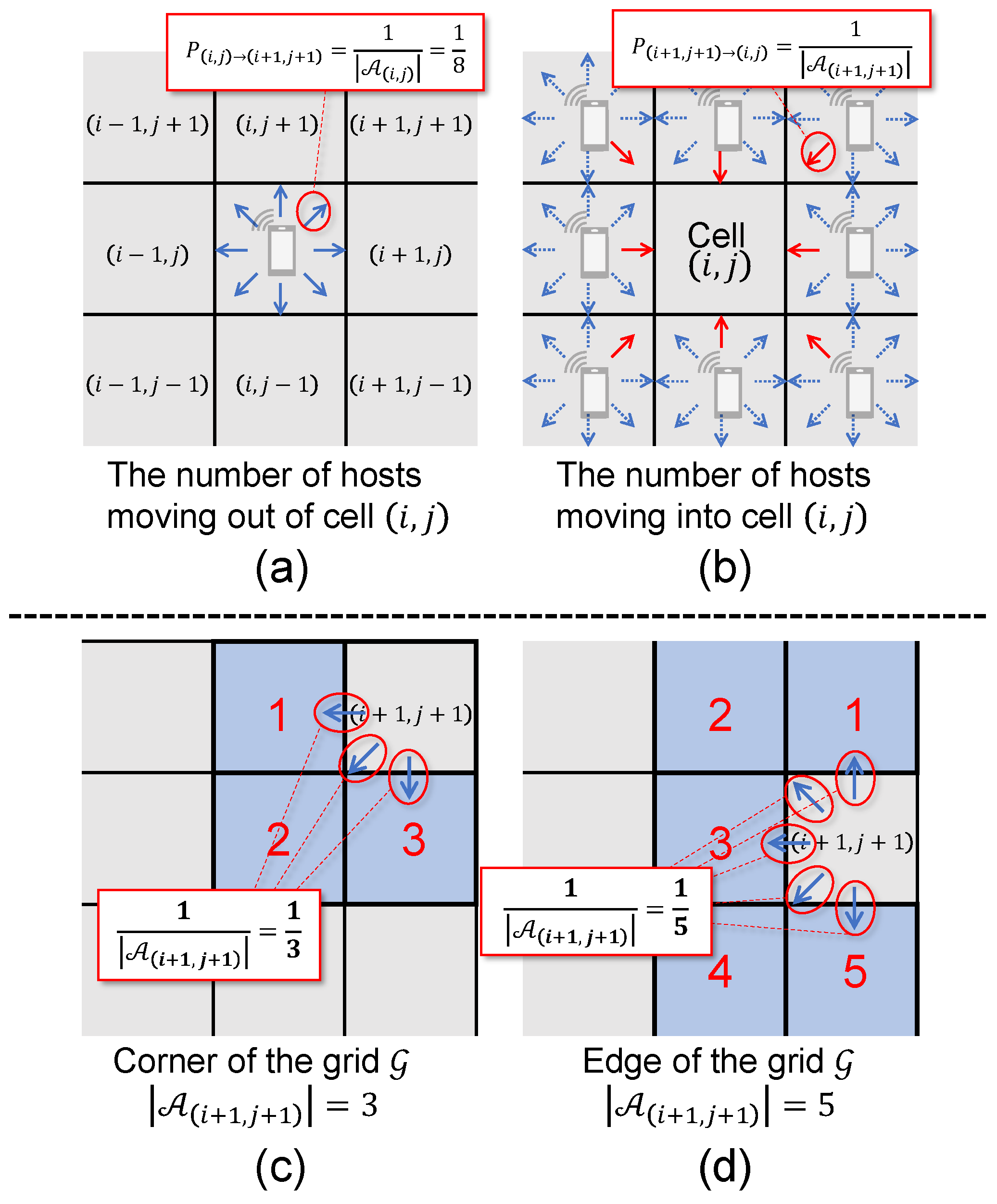
In the example shown in Figure 5, the probability that a host located in cell ( i , j ) moves to cell ( i + 1 , j + 1 ) is 1 / 8 (Figure 5a). This is because the size of the mobility neighborhood A ( i , j ) is 8. Furthermore, the probability of moving from cell ( i + 1 , j + 1 ) to cell ( i , j ) depends on A ( i + 1 , j + 1 ) . As illustrated in Figure 5c,d, if cell ( i + 1 , j + 1 ) is located at a corner of the grid G , then | A ( i + 1 , j + 1 ) | = 3 (Figure 5c), and if it is on an edge of the grid, then | A ( i + 1 , j + 1 ) | = 5 (Figure 5d); otherwise, | A ( i + 1 , j + 1 ) | = 8 .

4.2.2. Hotspot-Aware Movement Strategy

The hotspot-aware movement strategy adjusts the movement probability P ( i , j ) ( m , n ) based on the directional similarity between the host’s movement direction and that of nearby hotspots. In this strategy, the movement probability from cell ( i , j ) G to an adjacent cell ( m , n ) A ( i , j ) is defined as
P ( i , j ) ( m , n ) = W ( i , j ) ( m , n ) ( k , l ) A ( i , j ) W ( i , j ) ( k , l ) ,
where W ( i , j ) ( m , n ) denotes the total movement weight from cell ( i , j ) to ( m , n ) , obtained by aggregating the directional influence of all hotspots. Equation (8) represents the normalization process that converts directional similarity scores into a valid probability distribution over the set of candidate movement directions. The total movement weight W ( i , j ) ( m , n ) is calculated as
W ( i , j ) ( m , n ) = ( q , r ) Q w ( i , j ) ( m , n ) ( q , r ) ,
where w ( i , j ) ( m , n ) ( q , r ) denotes the cosine similarity-based weight associated with hotspot ( q , r ) , which will be defined later, and Q denotes the set of hotspots. Each hotspot is represented by its fixed coordinate ( q , r ) N 2 .
The cosine similarity-based weight w ( i , j ) ( m , n ) ( q , r ) is calculated as follows. Let V denote the set of movement vectors, which represents the possible directions that a host can take from a given cell. The movement vector set V is given by
V = ( 1 , 1 ) , ( 0 , 1 ) , ( 1 , 1 ) , ( 1 , 0 ) , ( 1 , 0 ) , ( 1 , 1 ) , ( 0 , 1 ) , ( 1 , 1 ) .
In addition, to capture the directional bias toward a specific hotspot ( q , r ) Q , we define the direction vector h ( i , j ) ( q , r ) from cell ( i , j ) G to the hotspot as follows:
h ( i , j ) ( q , r ) = ( q i , r j ) .
The cosine similarity CosSim ( v , h ( i , j ) ( q , r ) ) between movement vector v = ( m i , n j ) V and hotspot h ( i , j ) ( q , r ) Q is defined as
CosSim ( v , h ( i , j ) ( q , r ) ) = v · h ( i , j ) ( q , r ) v · h ( i , j ) ( q , r ) + ϵ ,
where ϵ denotes a small constant to avoid division by zero. With this cosine similarity, the cosine similarity-based weight w ( i , j ) ( m , n ) ( q , r ) in (9), representing the directional weight from cell ( i , j ) to ( m , n ) with respect to hotspot ( q , r ) , is given by
w ( i , j ) ( m , n ) ( q , r ) = max CosSim ( v , h ( i , j ) ( q , r ) ) h ( i , j ) ( q , r ) , 0 + 1 | A ( i , j ) | .
The term 1 | A ( i , j ) | ensures that there remains a small probability of moving in any direction, thereby incorporating an element of randomness while still achieving directional movement. In addition, the cosine similarity is scaled by h ( q , r ) ( q , r ) so that the influence of distant hotspots becomes smaller. This reflects the intuition that a host is less likely to move toward a hotspot that is located farther away.
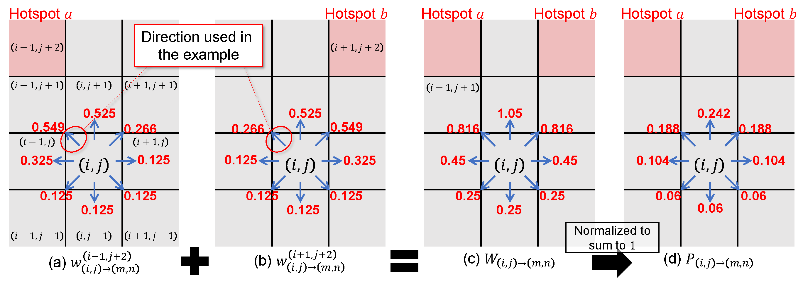
Figure 6 illustrates how to compute P ( i , j ) ( m , n ) in one concrete setting, where the host is at ( i , j ) G and there are two hotspots Q = { a , b } = { ( i 1 , j + 2 ) , ( i + 1 , j + 2 ) } . For ( i , j ) , the direction vectors to the hotspots are
h ( i , j ) ( i 1 , j + 2 ) = ( 1 , 2 ) , h ( i , j ) ( i + 1 , j + 2 ) = ( 1 , 2 ) .
As an example, consider the direction ( i , j ) ( i 1 , j + 1 ) whose movement vector is v = ( 1 , 1 ) . The cosine similarities used in (10) are then computed as
CosSim v , h ( i , j ) ( i 1 , j + 2 ) = v · h ( i , j ) ( i 1 , j + 2 ) v h ( i , j ) ( i 1 , j + 2 ) + ϵ = 1 · ( 1 ) + 1 · 2 2 · 5 + ϵ = 3 10 + ϵ 0.949 , CosSim v , h ( i , j ) ( i + 1 , j + 2 ) = 1 10 + ϵ 0.316 .
Substituting these into (10) yields the per-hotspot weights for this movement direction, which are then accumulated into the total weight:
w ( i , j ) ( i 1 , j + 1 ) ( i 1 , j + 2 ) = max 0.949 5 , 0 + 1 | A ( i , j ) | = 0.424 + 1 8 0.549 , w ( i , j ) ( i 1 , j + 1 ) ( i + 1 , j + 2 ) = max 0.316 5 , 0 + 1 | A ( i , j ) | = 0.141 + 1 8 0.266 .
Repeating this for all v V yields the values in Figure 6a for hotspot ( i 1 , j + 2 ) and in Figure 6b for hotspot ( i + 1 , j + 2 ) . We then sum the per-hotspot weights via (9) to obtain the total weight for each movement vector. For v = ( 1 , 1 ) ,
W ( i , j ) ( i 1 , j + 1 ) = ( q , r ) Q w ( i , j ) ( i 1 , j + 1 ) ( q , r ) = 0.549 + 0.266 0.816 ,
as shown in Figure 6c. Finally, we normalize the total weights over all ( m , n ) A ( i , j ) according to (8) to derive the movement probabilities. As an example, for the movement direction ( i , j ) ( i 1 , j + 1 ) , we obtain
P ( i , j ) ( i 1 , j + 1 ) = W ( i , j ) ( i 1 , j + 1 ) ( k , l ) A ( i , j ) W ( i , j ) ( k , l ) = 0.816 4.33 0.188 ,
as illustrated in Figure 6d. Applying the same procedure to all directions produces the full distribution of movement probabilities shown in the figure. Equation (8) is derived from these steps, and the resulting ODEs are obtained by substituting it into (4)–(6).

5. Numerical Evaluations

In the evaluation, we examine how the infection dynamics of mobile hosts mobile hosts vary under different movement models. Specifically, we substitute (7) (random movement) and (8) (proposed hotspot-aware movement) into the ODEs (4)–(6), and compare the resulting dynamics.

5.1. Model

We conduct numerical calculations to discuss the impact of hotspot configurations. In the numerical calculations, we use an HP Z8 G4 Workstation (HP Inc., Palo Alto, CA, USA) with an Intel Xeon Gold 5122 (Intel Corporation, Santa Clara, CA, USA) 3.60 GHz and 96 GB memory, running Ubuntu 22.04. In order to obtain solutions of our proposed model, we calculate the ODEs (4)–(6) using MATLAB R2024b [28].
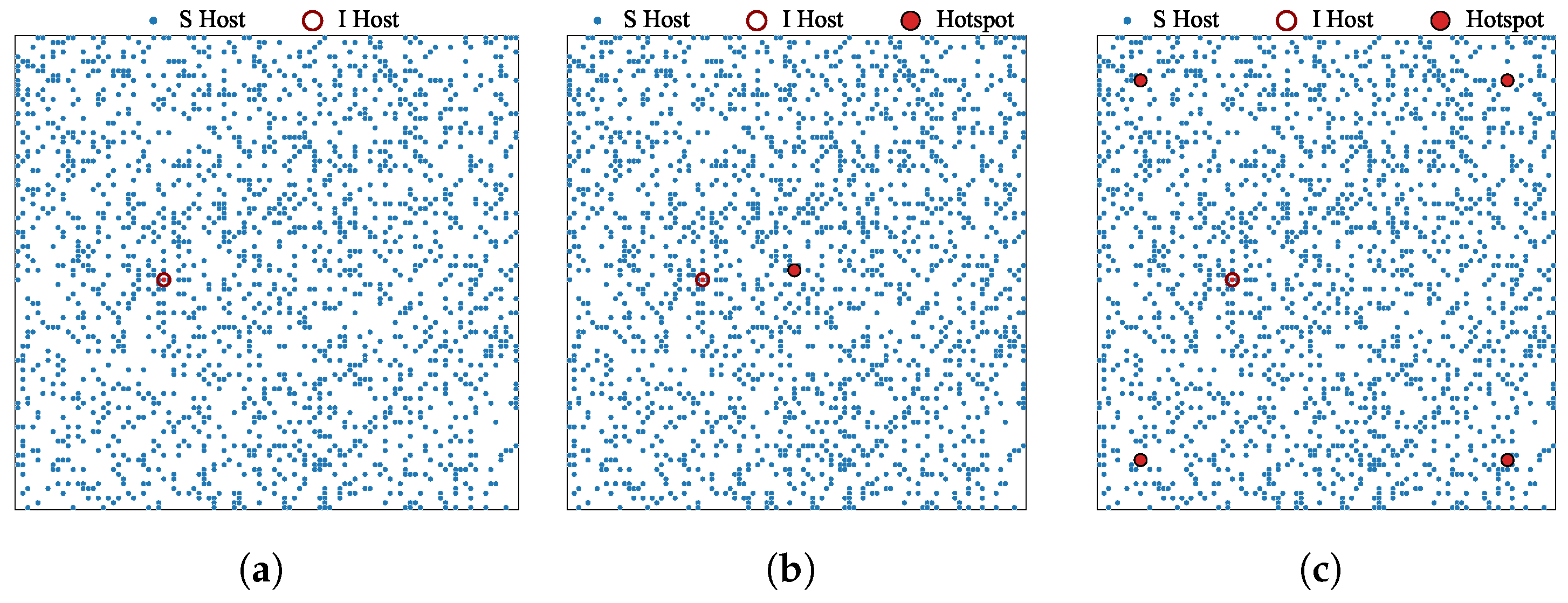
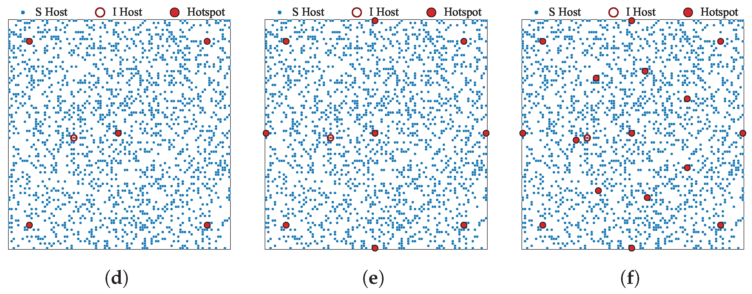
Table 1 summarizes the system parameters and their values used in this paper. The total number of hosts H is set to 2000, and the target area is divided into 100 × 100 cells. The set Q represents the coordinates of fixed hotspot locations, which serve as targets for biased movement. To focus on the behavioral differences introduced by the movement model, we set α in the range from 0.03 to 0.1, while both β and γ are fixed at 0.1. These values are chosen experimentally to observe how malware spreads in the network under both random and hotspot-aware movement. We set the initial condition as S ( 0 ) = 1999 , I ( 0 ) = 1 , and R ( 0 ) = 0 , where all vulnerable hosts are randomly distributed, and a single infected host is placed at position ( 29 , 51 ) .
The initial states of the calculations, illustrating the hotspot configurations, are shown in Figure 7. To evaluate the effect of hotspot placement, we consider six scenarios: (a) no hotspots, (b) a single hotspot located at the center, (c) four hotspots placed near the corners of the area, and (d)–(f) configurations with five or more hotspots. For scenarios involving more than four hotspots, the hotspot positions are chosen to maximize the pairwise distances among them, thereby enhancing spatial dispersion.

5.2. Result

5.2.1. Impact of Malware Infection Rate α

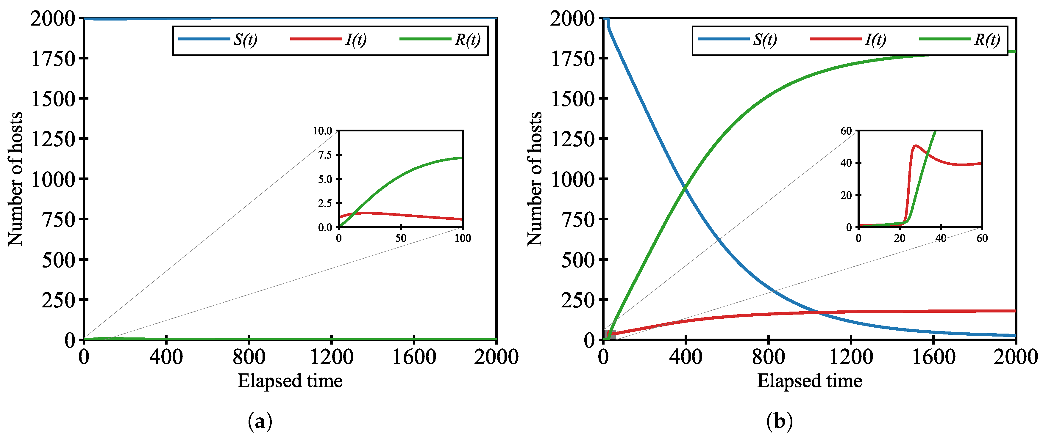
Figure 8 presents the numerical results under a low infection rate setting (i.e., α = 0.05 ), comparing two scenarios: one without any hotspots (Figure 8a) and another with a single hotspot placed at the center of the area (Figure 8b). The initial positions of the vulnerable hosts, the single infected host, and the hotspot(s) are illustrated in Figure 7a,b. Each plot shows the number of hosts in each state (i.e., S, I, and R) as a function of elapsed time. Additionally, the figures include an inset that magnifies the early-stage spread of infection, providing a detailed view of the initial dynamics that may not be clearly visible at full scale.
As shown in Figure 8a, in the no-hotspot case, although a slight increase in infections occurs at an early stage, the malware fails to propagate through the network. The infection quickly stabilizes, and the total number of infected hosts remains close to zero. This suggests that, under low infection rates, the lack of spatial convergence among hosts leads to limited contact opportunities between infected and susceptible hosts, thereby suppressing malware diffusion.
In contrast, under the proposed hotspot-aware movement strategy with a single hotspot placed at the center, the infection dynamics differ significantly. As shown in Figure 8b, the number of infected hosts exhibits a delayed onset followed by a rapid increase. This is due to the spatial aggregation of hosts around the hotspot, which raises the likelihood of contact between infected and susceptible individuals. As a result, even with a low infection rate, the elevated local density facilitates large-scale malware diffusion.
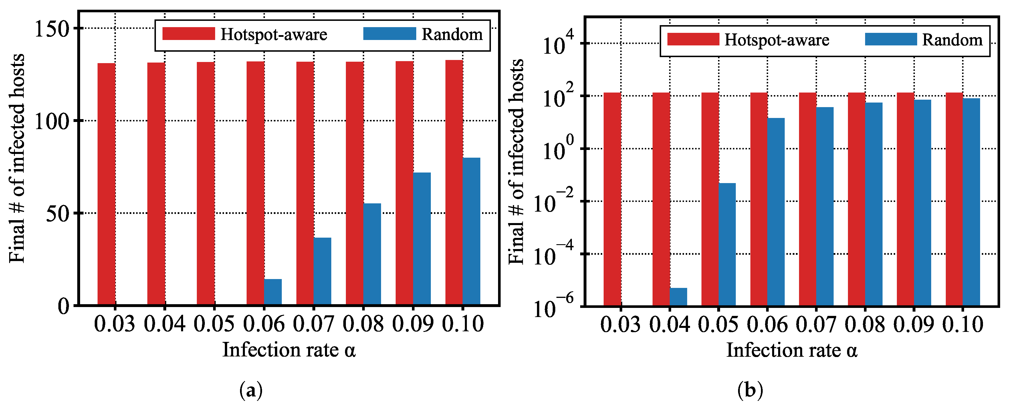
Figure 9 presents the number of infected hosts at 500 time units for various values of the infection rate α ranging from 0.03 to 0.1, comparing the proposed hotspot-aware movement strategy with the conventional random movement model. In both Figure 9a,b, the horizontal axis represents the infection rate α , while the vertical axis shows the number of infected hosts at a fixed time point. Figure 9a uses a linear scale to show absolute differences in infection counts, whereas Figure 9b adopts a logarithmic scale to better highlight behavior under low-infectivity conditions.
As shown in the figure, the hotspot-aware movement strategy significantly accelerates malware propagation even when the infection rate is low. For example, even at α = 0.03 , the number of infected hosts exceeds 600 under the hotspot-aware movement strategy, indicating that spatial concentration due to hotspot attraction can sustain transmission despite limited infectivity. In contrast, the random movement strategy shows virtually no spread at this infection level, with the number of infected hosts remaining close to zero.
These results indicate that the developed model produces consistent behaviors under the assumed conditions. Specifically, biased mobility patterns appear to have a substantial impact on malware diffusion dynamics. By promoting aggregation around hotspots, the proposed hotspot-aware movement strategy likely enhances local density and may increase the likelihood of contact between infected and susceptible hosts.

5.2.2. Impact of the Number of Hotspots

We then investigate how the number and spatial distribution of hotspots affect malware propagation dynamics. Figure 10 shows the number of hosts in each state as a function of the time elapsed, where the infection rate α = 0.1 . The hotspot configurations in Figure 10a–f correspond to the initial states shown in Figure 7a–f, respectively.
As shown in Figure 10a, when no hotspots are present, the infection spreads slowly and stabilizes at a relatively low level. In this case, since host movement is completely random, spatial convergence does not occur, and contacts between infected and susceptible hosts are limited. Figure 10b–f show that when one or more hotspots are introduced, the infection spreads more quickly and reaches a higher peak. Hotspots promote the local aggregation of hosts, increasing density and making transmission easier. When four or more hotspots are placed (Figure 10c–f), the infection dynamics become more complex: multiple peaks appear, and the total number of infected hosts increases further. These results suggest that having multiple attractive points leads to repeated clustering and sustained propagation in different areas.
In summary, the number of hotspots significantly affects both the speed and scale of malware diffusion. While one hotspot is enough to accelerate the spread compared to the random case, multiple hotspots allow repeated reinfection and result in higher saturation. These findings indicate that, in addition to infection rates, spatial movement patterns and hotspot density should be considered when modeling or preventing malware spread in wireless networks.
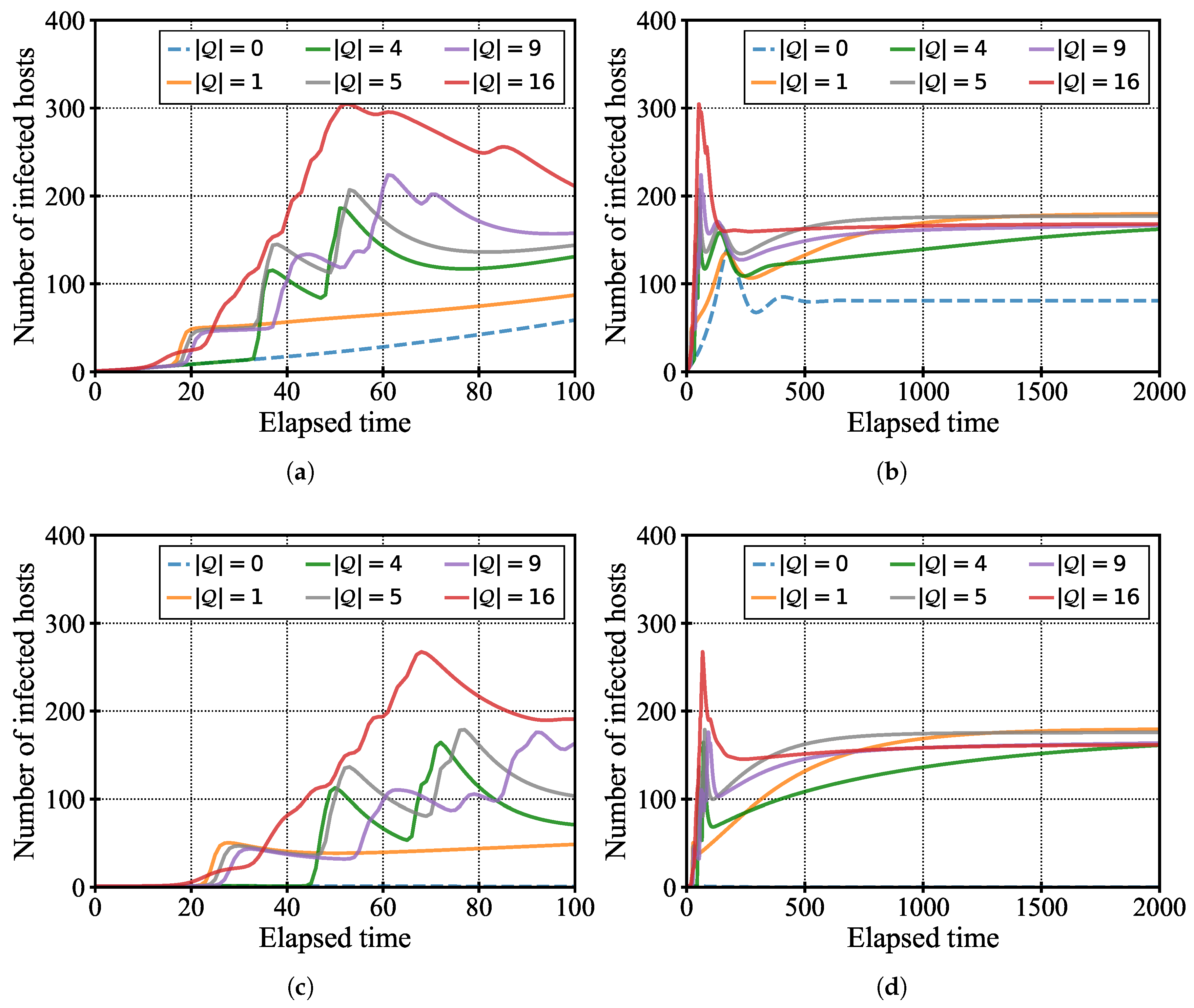
To further analyze the impact of hotspot placement on malware propagation, we compare six different hotspot configurations under fixed infection rates of α = 0.1 and α = 0.05 . Figure 11 shows the number of infected hosts under both infection rates, with early-stage and full-scale results shown in Figure 11a–d.
In the early-stage results (Figure 11a,c), we find that a greater number of hotspots tends to produce higher infection peaks in the early phase. The infection rises more quickly when hotspots are placed close together, followed by the case with a single hotspot at the center, and then by configurations with more dispersed layouts, such as center plus corners. This indicates that initial clustering is more likely when hosts are drawn toward nearby hotspots. Additionally, configurations with many hotspots often exhibit multiple infection peaks, suggesting that periodic re-clustering of hosts occurs over time. Such dynamic behavior resembles real-world urban mobility, which is often non-uniform and time-varying.
From the long-term results (Figure 11b,d), we observe that the configuration with a single hotspot placed at the center ultimately produces the highest total number of infected hosts. This indicates that a centrally located hotspot functions as a stable attractor, maintaining local density and facilitating persistent infection over time. In contrast, increasing the number of hotspots does not necessarily result in a proportional increase in infections. This suggests that widely dispersed attraction points may actually reduce opportunities for dense contact at any one location.
Even when the infection rate is lowered to α = 0.05 , the total number of infected hosts eventually reaches a level similar to that under α = 0.1 . This is because hosts continue to gather around hotspots over time, sustaining the infection. However, the peak number of infected hosts is lower, and the infection grows more slowly. These results emphasize that spatial aggregation plays a key role in sustaining transmission, even under low infectivity conditions. In other words, infection dynamics are not driven by high infectivity alone but also by localized density caused by biased movement. Therefore, hotspot-aware mobility must be considered even in scenarios where the infection risk is relatively low.

6. Discussion

We discuss the potential and limitations of the proposed model across the following key dimensions: modeling fidelity, data integration, computational scalability, and practical applicability.

6.1. Modeling Fidelity

The proposed framework adopts a macroscopic view of malware diffusion, focusing on aggregated infection dynamics rather than the behavior of individual threats. While this abstraction enables tractable analysis with ODEs, it also introduces approximations. For instance, host positions are tracked only at the cell level, which neglects finer spatial variation. Similarly, parameters such as the infection rate α , elimination rate β , discovery rate γ , and mobility rate μ are fixed constants. These assumptions simplify analysis but may overlook time-varying or context-dependent effects, such as higher mobility near hotspots or increased elimination rates during patch campaigns. A promising direction for future work is to refine the spatial resolution or to incorporate hybrid methods, such as without significantly increasing computational complexity, agent-based simulation, to better capture local movement dynamics.
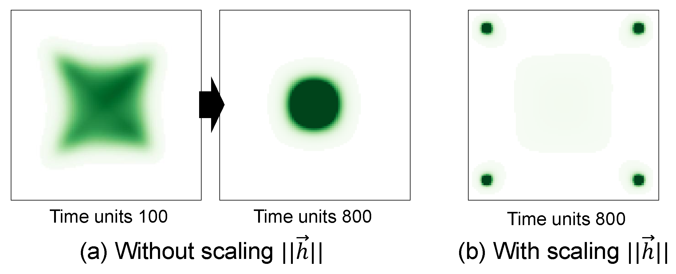
Another limitation lies in the design of the cosine-similarity-based mobility weight. In the current formulation in (10), the term 1 / | A ( i , j ) | preserves a baseline random movement, and the inverse of the Euclidean norm h ( i , j ) ( q , r ) serves as a simple distance scaling factor. To illustrate the impact of this distance scaling, we compare results with and without h ( i , j ) ( q , r ) in (10) (see Figure 12 where hotspots are located at the four corners). As shown in Figure 12a, without distance scaling, hosts move toward hotspots with equal strength regardless of their location. Consequently, instead of moving toward the four hotspots, all hosts converge near the center. In contrast, with distance scaling (Figure 12b), hosts tend to cluster around the hotspot regions.
The linear inverse-distance scaling is heuristic, and more refined decay functions could better capture how the influence of hotspots attenuates with distance. For example, (10) could be replaced by the following power-law variant:
CosSim ( v , h ( i , j ) ( q , r ) ) h ( i , j ) ( q , r ) κ ,
or by an exponential decay formulation:
CosSim ( v , h ( i , j ) ( q , r ) ) · exp λ h ( i , j ) ( q , r ) ,
where κ > 0 and λ > 0 are tunable decay parameters. These alternatives allow for more flexible modeling of distance-based attenuation in mobility, potentially leading to more realistic simulations of spatial dynamics. Furthermore, ablation studies (e.g., removing the baseline term or comparing different normalization methods) would help clarify the sensitivity of infection outcomes to weight design. We leave these directions for future work.

6.2. Empirical Data Integration

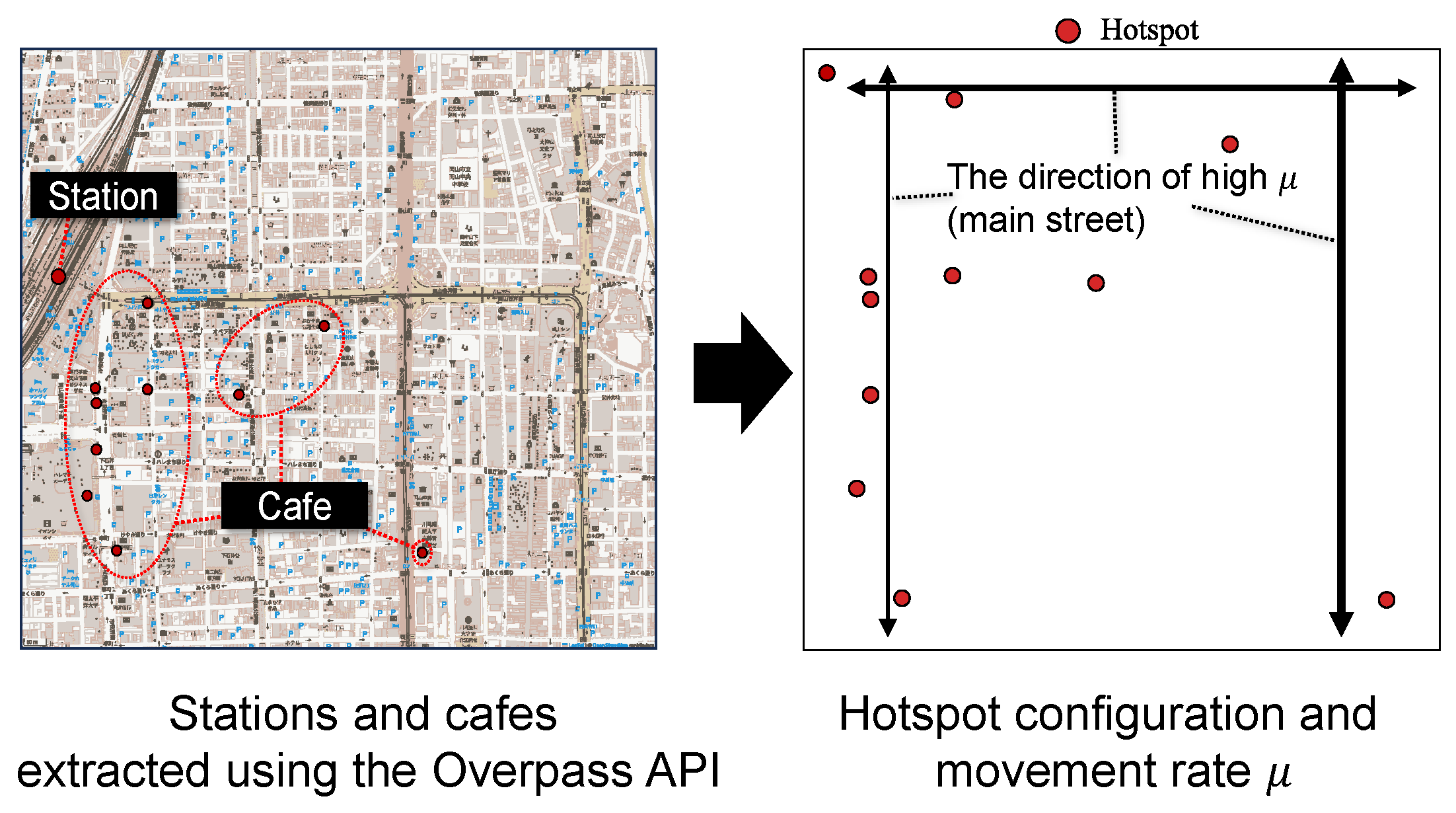
In this paper, the hotspot configurations are designed as synthetic patterns (e.g., center-aligned and corner-based) to illustrate the contrasting effects. These were not grounded in sociological studies of human mobility. As a future direction, we plan to incorporate empirical data to improve realism. For instance, we will be able to use the Overpass API [29] or CRAWDAD [30] to extract real-world locations such as cafes and train stations around a selected urban area as shown in Figure 13. These data can inform more realistic hotspot placement by identifying regions where human activity is naturally concentrated.
Urban structures such as roads and building layouts also influence how mobile hosts move. Therefore, it is important to incorporate spatial heterogeneity in movement rates μ across the grid. For example, higher mobility along major streets can be modeled by assigning higher μ values in those directions as shown in Figure 13. Furthermore, Song et al. [9] analyzed large-scale mobile phone trajectory data and demonstrated that human mobility is highly regular and predictable, with up to 93% predictability on average. This evidence suggests that real human movement is far from random, and thus incorporating real mobility traces would enhance model fidelity.

6.3. Computational Scalability

The current grid-based formulation scales nearly quadratically with the number of cells, which may limit applicability to urban-scale networks. Approximation methods, such as mean-field or reduced-order modeling, represent promising directions to reduce computational burden while maintaining essential dynamics. In fact, we have previously applied mean-field based modeling to botnet malware diffusion [31] and proposed approximate methods for large grid-based simulations [32]. These experiences suggest that similar approaches could make the present model applicable to large-scale environments.

6.4. Practical Applicability and Policy Insights

The persistence of infection under low infectivity emphasizes the importance of spatial aggregation in both digital and physical domains. In cybersecurity, hotspot-aware countermeasures, such as prioritizing patch distribution to devices in dense communication areas or segmenting networks around central hubs, could suppress persistent malware clusters. In public health, analogous strategies include temporary movement restrictions or the targeted allocation of resources around gathering points. More broadly, incorporating time-varying parameters, conducting theoretical analyses of equilibrium thresholds, and validating results against real mobility traces will strengthen both the theoretical rigor and the practical relevance of this work.

7. Conclusions and Future Work

7.1. Conclusions

This paper presents a novel deterministic epidemic model that captures malware propagation in wireless mobile networks by incorporating spatially biased mobility toward predefined hotspots. Unlike conventional approaches that assume uniform random movement, the proposed model introduces movement probabilities that are adjusted based on directional similarity, quantified by cosine similarity between a host’s movement and the direction of nearby hotspots. By integrating these movement probabilities into a system of ODEs, we developed a modeling framework that more accurately reflects realistic mobility patterns observed in urban environments.
We evaluated the proposed model through numerical calculations and compared it with the random movement strategy, considering six hotspot configurations (0, 1, 4, 5, 9, and 16 hotspots) under two infection rate settings: α = 0.1 and α = 0.05 . Even under a lower infection rate, the total number of infected hosts eventually reaches a level comparable to that under the higher rate, as hosts continued to aggregate around hotspots over time. However, the infection spread more slowly, and the peak number of infected hosts was lower. These results indicate that malware propagation is not driven by infectivity alone but also by local density caused by biased movement toward hotspots, which plays a critical role in sustaining transmission.
Furthermore, in the early stage, a greater number of hotspots led to faster infection spread and higher peaks due to rapid spatial clustering. The infection rose most quickly when hotspots were placed close together, followed by the case with a single central hotspot, and then by configurations with more dispersed layouts such as center plus corners. In contrast, in the long term, the configuration with a single centrally located hotspot produced the highest total number of infected hosts. This suggests that such a hotspot acts as a stable attractor, maintaining local density and facilitating persistent infection.
These findings highlight the critical role of mobility structure in epidemic modeling. Incorporating spatial directionality through cosine similarity enabled our model to simulate localized infection clusters, which more closely resemble real-world diffusion patterns seen in mobile or IoT environments. This suggests that hotspot-aware mobility is a key factor in understanding and predicting malware outbreaks, especially in densely populated or high-traffic areas such as campuses, train stations, or commercial zones.
Beyond theoretical insights, these findings carry societal relevance: the persistence of infection under low infectivity highlights risks for both public health (e.g., sustained outbreaks in crowded urban areas) and cybersecurity (e.g., IoT malware spreading in dense communication zones). These results underscore the importance of hotspot-aware policies and preventive strategies, such as targeted resource allocation in public health and prioritized patch distribution in cybersecurity. In this way, our model contributes not only to theoretical understanding but also to practical considerations for policy and risk management.

7.2. Future Work

Future research will proceed along three major directions.
First, we aim to enhance the realism and adaptability of the model by integrating empirical mobility data and refining parameter dynamics. This includes incorporating real hotspot distributions, calibrating spatially heterogeneous μ values, and introducing time-varying or context-dependent parameters such as increased β during patching campaigns. We also plan to explore alternative distance decay functions and conduct ablation studies on the cosine similarity-based mobility weight.
Second, we will investigate the theoretical foundations of the model. Specifically, we plan to analyze the equilibrium properties of the ODE system and derive threshold conditions such as the basic reproduction number ( R 0 ), which is essential in epidemiological modeling. These efforts will extend the scope of the model beyond numerical simulations and enhance its analytical rigor.
Third, we will assess scalability and practical applicability by comparing the proposed ODE framework with agent-based and stochastic models (e.g., continuous-time Markov chain). This comparison will guide the selection of appropriate modeling approaches. Furthermore, we will explore practical countermeasures such as hotspot-aware patching and mobility control to connect theoretical insights with actionable strategies for cybersecurity and public health.

Author Contributions

Conceptualization, H.M. and K.H.; methodology, H.M. and K.H.; software, H.M.; validation, T.K.; formal analysis, T.K.; investigation, H.M. and T.K.; resources, K.H.; data curation, H.M.; writing—original draft preparation, H.M. and K.H.; writing—review and editing, T.K.; visualization, H.M. and K.H.; supervision, T.K.; project administration, K.H.; funding acquisition, T.K. All authors have read and agreed to the published version of the manuscript.

Funding

This research was supported by JSPS KAKENHI Grant Number 23K11077.

Data Availability Statement

Data are available from the authors upon request.

Conflicts of Interest

The authors declare no conflicts of interest.

References

  1. Cisco. Cisco Annual Internet Report (2018–2023) White Paper. Technical Report. 2018. Available online: https://www.cisco.com/c/en/us/solutions/collateral/executive-perspectives/annual-internet-report/white-paper-c11-741490.html (accessed on 1 August 2025).
  2. Lonzetta, A.M.; Cope, P.; Campbell, J.; Mohd, B.J.; Hayajneh, T. Security Vulnerabilities in Bluetooth Technology as Used in IoT. J. Sens. Actuator Netw. 2018, 7, 28. [Google Scholar] [CrossRef]
  3. Ronen, E.; Shamir, A.; Weingarten, A.O.; O’Flynn, C. IoT Goes Nuclear: Creating a ZigBee Chain Reaction. In Proceedings of the 2017 IEEE Symposium on Security and Privacy (SP), San Jose, CA, USA, 22–26 May 2017; pp. 195–212. [Google Scholar] [CrossRef]
  4. Milanovic, A.F.; Melikov, N.; Legezo, D. Skygofree: Following in the Footsteps of HackingTeam. 2018. Available online: https://securelist.com/skygofree-following-in-the-footsteps-of-hackingteam/83603/ (accessed on 28 June 2025).
  5. Zeng, W.; Zhang, C.; Liang, X.; Xia, J.; Lin, Y.; Lin, Y. Intrusion detection-embedded chaotic encryption via hybrid modulation for data center interconnects. Opt. Lett. 2025, 50, 4450–4453. [Google Scholar] [CrossRef]
  6. Kermack, W.O.; McKendrick, A.G. A contribution to the mathematical theory of epidemics. Proc. R. Soc. Lond. Ser. 1927, 115, 700–721. [Google Scholar]
  7. Gonzalez, G.; Larraga, M.E.; Alvarez-Icaza, L.; Gomez, J. Bluetooth Worm Propagation in Smartphones: Modeling and Analyzing Spatio-Temporal Dynamics. IEEE Access 2021, 9, 75265–75282. [Google Scholar] [CrossRef]
  8. Miura, H.; Abukawa, S.; Kimura, T.; Hirata, K. Modeling of malware diffusion with mobile devices in intermittently connected networks. In Proceedings of the 2022 Asia-Pacific Signal and Information Processing Association Annual Summit and Conference (APSIPA ASC), Chiang Mai, Thailand, 7–10 November 2022; pp. 1756–1759. [Google Scholar] [CrossRef]
  9. Song, C.; Qu, Z.; Blumm, N.; Barabási, A.L. Limits of Predictability in Human Mobility. Science 2010, 327, 1018–1021. [Google Scholar] [CrossRef]
  10. Toole, J.L.; Lin, Y.R.; Muehlegger, E.; Shoag, D.; González, M.C. Coupling human mobility and social ties. J. R. Soc. Interface 2015, 12, 20141128. [Google Scholar] [CrossRef] [PubMed]
  11. Fan, Y.; Dong, Y.; Xu, J.; Chawla, N.V. Correlation between social proximity and mobility similarity. Sci. Rep. 2017, 7, 11975. [Google Scholar] [CrossRef] [PubMed]
  12. Memon, M.W.; Singh, A.V.; Raj, R.G. Analysis and Implementation of Human Mobility Behavior Using Similarity Analysis Based on Co-Occurrence Matrix. Sensors 2022, 22, 9898. [Google Scholar] [CrossRef] [PubMed]
  13. LeCun, Y.; Bengio, Y.; Hinton, G. Deep learning. Nature 2015, 521, 436–444. [Google Scholar] [CrossRef] [PubMed]
  14. Truong, T.C.; Zelinka, I. A Survey on Artificial Intelligence in Malware as Next-Generation Threats. Mendel 2019, 25, 27–34. [Google Scholar]
  15. Truong, T.C.; Diep, Q.B.; Zelinka, I. Artificial Intelligence in the Cyber Domain: Offense and Defense. Symmetry 2020, 12, 410. [Google Scholar] [CrossRef]
  16. Kudo, T.; Kimura, T.; Inoue, Y.; Aman, H.; Hirata, K. Stochastic modeling of self-evolving botnets with vulnerability discovery. Comput. Commun. 2018, 124, 101–110. [Google Scholar] [CrossRef]
  17. Shi, Y.; Davaslioglu, K.; Sagduyu, Y.E. Generative Adversarial Network in the Air: Deep Adversarial Learning for Wireless Signal Spoofing. IEEE Trans. Cogn. Commun. Netw. 2021, 7, 294–303. [Google Scholar] [CrossRef]
  18. Li, Y.; Wang, Y.; Wang, Y.; Ke, L.; Tan, Y. A feature-vector generative adversarial network for evading PDF malware classifiers. Inf. Sci. 2020, 523, 38–48. [Google Scholar] [CrossRef]
  19. Li, H.; Zhou, S.; Yuan, W.; Li, J.; Leung, H. Adversarial-Example Attacks Toward Android Malware Detection System. IEEE Syst. J. 2020, 14, 653–656. [Google Scholar] [CrossRef]
  20. Armis. BlueBorne Cyber Threat Impacts Amazon Echo and Google Home. 2017. Available online: https://www.armis.com/blog/blueborne-cyber-threat-impacts-amazon-echo-and-google-home/ (accessed on 28 June 2025).
  21. Armis. The Attack Vector “BlueBorne” Exposes Almost Every Connected Device. 2017. Available online: https://media.armis.com/PDFs/wp-blueborne-bluetooth-vulnerabilities-en.pdf (accessed on 28 June 2025).
  22. Ruge, J.; Pohlmann, J.K.; Holtz, T.; Hollick, M. Frankenstein: Advanced Wireless Fuzzing to Exploit New Bluetooth Escalation Targets. In Proceedings of the 29th USENIX Security Symposium (USENIX Security 20), Boston, MA, USA, 12–14 August 2020; USENIX Association: Berkeley, CA, USA, 2020; pp. 19–36. [Google Scholar]
  23. Xiao, X.; Fu, P.; Dou, C.; Li, Q.; Hu, G.; Xia, S. Design and analysis of SEIQR worm propagation model in mobile internet. Commun. Nonlinear Sci. Numer. Simul. 2017, 43, 341–350. [Google Scholar] [CrossRef]
  24. Shen, S.; Zhou, H.; Feng, S.; Liu, J.; Zhang, H.; Cao, Q. An Epidemiology-Based Model for Disclosing Dynamics of Malware Propagation in Heterogeneous and Mobile WSNs. IEEE Access 2020, 8, 43876–43887. [Google Scholar] [CrossRef]
  25. Okamura, H.; Kobayashi, H.; Dohi, T. Markovian modeling and analysis of Internet worm propagation. In Proceedings of the 16th IEEE International Symposium on Software Reliability Engineering (ISSRE’05), Chicago, IL, USA, 8–11 November 2005. [Google Scholar]
  26. Peng, S.; Wu, M.; Wang, G.; Yu, S. Propagation model of smartphone worms based on semi-Markov process and social relationship graph. Comput. Secur. 2014, 44, 92–103. [Google Scholar] [CrossRef]
  27. Peng, Z.; Zhang, Z.; Kong, X.; Liu, Z.; Liu, X. A movement-aware measure for trajectory similarity and its application for ride-sharing path extraction in a road network. Int. J. Geogr. Inf. Sci. 2024, 38, 1703–1727. [Google Scholar] [CrossRef]
  28. MATLAB. Available online: https://jp.mathworks.com/products/matlab.html (accessed on 15 June 2021).
  29. Olbricht, R. Overpass API. 2024. Available online: https://overpass-api.de/ (accessed on 22 August 2025).
  30. Kotz, D.; Henderson, T.; Abyzov, I. CRAWDAD: A Community Resource for Archiving Wireless Data at Dartmouth. 2004. Available online: https://crawdad.org (accessed on 24 August 2025).
  31. Miura, H.; Kimura, T.; Hirata, K. Deterministic epidemic modeling of future botnet malware with a contact process. IEICE Commun. Express 2021, 10, 295–300. [Google Scholar] [CrossRef]
  32. Miura, H.; Abukawa, S.; Kimura, T.; Hirata, K. Approximate modeling of malware diffusion on wireless mobile devices. In Proceedings of the 2023 Asia Pacific Signal and Information Processing Association Annual Summit and Conference (APSIPA ASC), Taipei, Taiwan, 31 October–3 November 2023; pp. 2144–2148. [Google Scholar] [CrossRef]
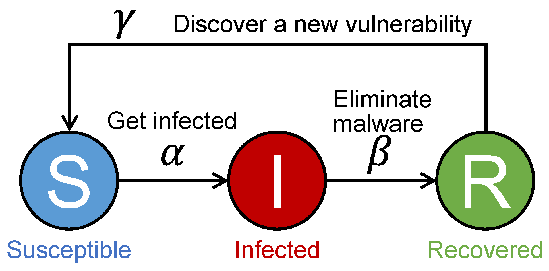
Figure 1. State transition of each host in the SIRS model.
Electronics 14 03528 g001
Figure 2. System model.
Electronics 14 03528 g002
Figure 3. The behavior of each host.
Electronics 14 03528 g003
Figure 4. Proposed movement strategy.
Electronics 14 03528 g004
Figure 5. Random movement strategy. (a) From an interior cell, each of the eight adjacent cells is selected with probability 1 / 8 . (b) Example of a move from the adjacent cells to ( i , j ) . (c) From a corner cell, each of the three adjacent cells is selected with probability 1 / 3 . (d) From an edge cell, each of the five adjacent cells is selected with probability 1 / 5 .
Electronics 14 03528 g005
Figure 6. Illustrative example of how to compute W ( i , j ) ( m , n ) and P ( i , j ) ( m , n ) , assuming two hotspots located at a = ( i 1 , j + 2 ) and b = ( i + 1 , j + 2 ) .
Electronics 14 03528 g006
Figure 7. Initial configurations of hosts and hotspots for the six scenarios considered in the experiment. In each scenario, one infected host is initially placed at cell ( 29 , 51 ) , while the remaining susceptible hosts are randomly distributed across the grid. Hotspots (if any) are positioned as follows: (a) no hotspots; (b) a single hotspot placed at ( 50 , 50 ) ; (c) four hotspots placed at ( 10 , 10 ) , ( 10 , 90 ) , ( 90 , 10 ) , and ( 90 , 90 ) ; (df) hotspots are arranged to maximize the pairwise distances among them.
Electronics 14 03528 g007aElectronics 14 03528 g007b
Figure 8. Time evolution of the number of hosts in each state (S, I, and R) under a low infection rate setting ( α = 0.05 ). (a) Scenario without any hotspots. (b) Scenario with a single hotspot placed at the center. The inset in each figure highlights the early-stage dynamics by zooming in on the shaded region.
Electronics 14 03528 g008
Figure 9. Comparison of the number of infected hosts at time step 500 for varying infection rates α (ranging from 0.03 to 0.1), comparing the proposed movement strategy with the conventional random movement model. (a) Results shown on a linear scale. (b) Results shown on a logarithmic scale to highlight behavior under low infection rates.
Electronics 14 03528 g009
Figure 10. Time evolution of the number of hosts in each state ( S ( t ) , I ( t ) , and R ( t ) ) under different hotspot configurations, with infection rate fixed at α = 0.1 . Each subfigure corresponds to a different number of hotspots: (a) 0 hotspots, (b) 1 hotspot, (c) 4 hotspots, (d) 5 hotspots, (e) 9 hotspots, (f) 16 hotspots. The corresponding initial configurations are shown in Figure 7a–f.
Electronics 14 03528 g010
Figure 11. Comparison of infection dynamics under different hotspot configurations for two infection rates. (a,b) The number of infected hosts over time with α = 0.1 (early-stage and full scale, respectively). (c,d) The same for α = 0.05 . The early-stage plots (a,c) represent the first 100 time units of the corresponding full scale plots.
Electronics 14 03528 g011
Figure 12. Comparison of host distribution with and without distance scaling in the mobility weight. (a) Without distance scaling, hosts move toward all hotspots with equal strength, resulting in convergence near the center. (b) With distance scaling, hosts tend to cluster around the hotspot regions.
Electronics 14 03528 g012
Figure 13. Real-world locations of hotspots (left) and their corresponding positions on a 100 × 100 simulation grid (right). The hotspot data, extracted using the Overpass API, include cafes and stations around a selected urban area. Based on this mapping, direction-specific movement rates μ can be adjusted to reflect urban structures such as roads.
Electronics 14 03528 g013
Table 1. List of system parameters.
ParametersDescriptionValue
HTotal number of hosts2000
N × M Total number of cells 100 × 100
| Q | Number of hotspots0, 1, 4, 5, 9, 16
α Malware infection rate [ 0.03 , 0.1 ]
β Malware elimination rate 0.1
γ Vulnerability discovery rate 0.01
μ Movement rate1
Disclaimer/Publisher’s Note: The statements, opinions and data contained in all publications are solely those of the individual author(s) and contributor(s) and not of MDPI and/or the editor(s). MDPI and/or the editor(s) disclaim responsibility for any injury to people or property resulting from any ideas, methods, instructions or products referred to in the content.