Abstract
To enhance the accuracy and precision of fault diagnosis and location for the collector lines in wind farms under complex operating conditions, an intelligent combined method based on CNN-LSTM and ICEEMDAN-PE-improved wavelet threshold denoising is proposed. A wind power plant model is established using the PSCADV46/EMTDC software. In response to the issue of indistinct fault current signal characteristics under complex fault conditions, a hybrid fault diagnosis model is constructed using CNN-LSTM. The convolutional neural network is utilized to extract the local time-frequency features of the current signals, while the long short-term memory network is employed to capture the dynamic time series patterns of faults. Combined with the improved phase-mode transformation, various types of faults are intelligently classified, effectively resolving the problem of fault feature extraction and achieving a fault diagnosis accuracy rate of 96.5%. To resolve the problem of small fault current amplitudes, low fault traveling wave amplitudes, and difficulty in accurate location due to noise interference in actual wind farms with high-resistance grounding faults, a combined denoising algorithm based on ICEEMDAN-PE-improved wavelet threshold is proposed. This algorithm, through the collaborative optimization of modal decomposition and entropy threshold, significantly improves the signal-to-noise ratio and reduces the root mean square error under simulated conditions with injected Gaussian white noise, stabilizing the fault location error within 0.5%. Extensive simulation results demonstrate that the fault diagnosis and location method proposed in this paper can effectively meet engineering requirements and provide reliable technical support for the intelligent operation and maintenance system of a wind farm.
1. Introduction
Within the context of carbon peaking strategies, wind energy has emerged as a critical component of power systems due to its clean attributes and abundant resources. However, large-scale wind farms face prominent operational challenges, particularly frequent collector line failures in complex environments. These failures not only compromise power generation efficiency but also threaten grid security and stability. Consequently, research on fault diagnosis and precise location technologies for collector lines holds significant engineering value: enhancing operational reliability and energy utilization efficiency of wind farms while serving as a critical technological enabler for scaling wind power deployment [1].
In the complex wind farm operation environment, the fault diagnosis and location of collector lines face many technical bottlenecks. In the field of wind farm collector line fault diagnosis, existing methods can be divided into traditional electrical characteristic-based methods and intelligent algorithm-driven methods, each with their own advantages and limitations in practical applications. In [2], a terminal grounding fault diagnosis method using metal sheath current/voltage signals is proposed for fault identification, which demonstrates certain effectiveness in simple cable network scenarios but remains unverified in terms of applicability to multi-branch cable networks. In [3], fault identification is realized by leveraging the sheath current characteristics of adjacent common ground laying high-voltage cables, but this method has obvious limitations in universality for other grounding methods such as cross interconnection. In [4,5], combined transfer learning and deep neural networks for robust intersubject EEG signal analysis demonstrate the effectiveness of intelligent algorithms in complex physiological signal processing. However, neither study is tailored to the specific challenges of wind farm collector line fault diagnosis, such as multi-branch network complexity and high-resistance fault signal processing, limiting their direct applicability to the scenario addressed in this research. In [6], the chaotic system, discrete wavelet transform (DWT), and convolutional neural network (CNN) are innovatively integrated to enhance feature recognition. Although the complexity of the model increases, the computational efficiency is reduced. In [7], incremental learning is employed with deep CNN (DCNN) to improve model generalization; however, the implementation of the incremental mechanism and the feasibility of edge device deployment require further exploration. In [8], bagging-integrated heterogeneous k-NN is adopted for diagnostic stability, yet challenges in real-time performance and interpretability remain. In [9,10], comprehensive reviews of existing technologies are presented, but they lack in-depth discussion on the deep integration of artificial intelligence with practical wind farm scenarios. This results in unresolved challenges in tackling multi-branch network complexity, achieving a balance between computational efficiency and diagnostic accuracy, and ensuring suitability for engineering applications—these drawbacks highlight the critical need for the CNN-LSTM hybrid framework proposed in this study.
In the field of cable fault location technology, existing methods, including traditional approaches like the impedance method and traveling wave method, as well as emerging technologies, exhibit distinct characteristics in practical applications. In [11], the zero-sequence impedance method optimized for distribution network fault location struggles with high-resistance fault scenarios—its accuracy remains limited, and harmonic interference from distributed generation remains unresolved, restricting reliability in complex operations. In [12], the double-ended traveling wave mode decomposition method proposed for UHV DC lines is constrained by signal synchronization errors, causing ±20% accuracy fluctuations in field tests, making it unsuitable for scenarios requiring stable precision. In [13], the combination of MUSIC algorithms and deep learning for submarine cable acoustic positioning brings innovative ideas to noise-resistant positioning, showcasing potential in enhancing stability under noisy conditions, though it is restricted by deep-sea noise environments and high deployment costs. In [14], Elaziz’s inductive wireless power transfer (IWPT) technology for low-voltage cables expands the technical pool for fault detection with its unique working principle, yet its safety suitability in high-voltage scenarios remains unverified. In [15], optical time-domain reflectometer (OTDR) technology, while providing a non-intrusive detection approach based on light wave propagation characteristics, suffers over 35% accuracy attenuation in complex environments. To address these limitations across both traditional and emerging methods in complex scenarios such as multi-branch networks and high-resistance faults, this study focuses on developing a robust fault location strategy tailored to practical application needs.
To address the critical problems of fault type misidentification and noise interference in wind farm collector lines, this study develops an integrated framework with three key innovations. To resolve the difficulty in extracting complex fault features where traditional methods struggle to capture local time-frequency characteristics and dynamic timing rules of fault current, a CNN-LSTM hybrid fault diagnosis model is proposed, leveraging the feature extraction capabilities of CNN and LSTM to enable accurate intelligent fault classification; To resolve issues of poor signal quality under noise interference, especially weak high-resistance fault signals and strong noise interference, an ICEEMDAN-PE-wavelet joint noise reduction algorithm is proposed; To resolve the problem of positioning inaccuracy caused by wave velocity fluctuation and signal distortion in traditional fault positioning methods, the above fault diagnosis results and denoised signals are applied to fault positioning: with fault diagnosis results as a priori information, wave velocity and wavelet parameters are adaptively calibrated, and wave head time is corrected by combining noise reduction signal reconstruction, thereby improving the accuracy of fault positioning.
2. Simulation Modeling and Analysis of Wind Farm Collector Line
The research object of this paper is Tongyu Wind Farm in Jilin Province, China. Based on the main wiring diagram and related original data of the wind farm, the simulation model of the wind farm collector line is established by PSCADV46/EMTDC software. As shown in Figure 1.
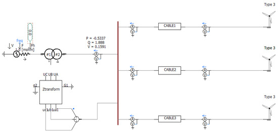
Figure 1.
Simulation model of the wind farm collector line.
The main grid of the wind farm is connected to the power system through a 220 kV/35 kV step-up transformer. The voltage level of the wind farm collector network is 35 kV, consisting of three cable lines of different lengths. Each cable line has multiple doubly fed induction generators (DFIGs) connected through a 0.69 kV/35 kV cabinet transformer. The neutral point of the 35 kV system is extracted by a Z-type grounding transformer and grounded by small resistance. The main part of the modeling is introduced as follows.
2.1. Modeling of the Wind Turbine
The wind turbine uses a 2 MW doubly fed induction generator. To prevent low voltage ride-through issues caused by external faults, the wind turbine model is equipped with a crowbar protection module and configured with low voltage ride-through (LVRT) strategies [16]. The DFIG simulation structure diagram is shown in Figure 2.
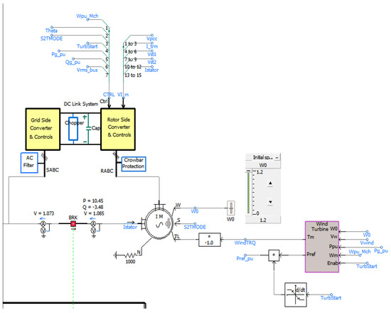
Figure 2.
DFIG simulation structure diagram.
2.2. Grounding Mode and Modeling of the Wind Farm
In the wind farm collector grid, the cable is used to replace the overhead line, and the single-phase grounding capacitive current of the cable line is much larger than that of the overhead line. If the neutral point is grounded through the arc suppression coil, the arc at the fault point is often unable to be eliminated, and the resulting dangerous resonance overvoltage cannot be suppressed. According to NB/T 31026 ‘Wind Farm Design Specifications’ [17] and the State Grid’s key measures to prevent large-scale wind power off-grid [18], in order to ensure the rapid removal of faults on the collector line and prevent large-scale off-grid of wind turbines, most of the actual wind farms use Z-type grounding transformers grounded by small resistance. The connection mode of the Z-type grounding transformer is shown in Figure 3.
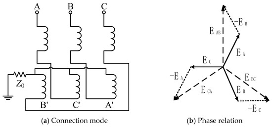
Figure 3.
Zn, yn11 grounding transformer.
The relationship between the magnetizing reactance and the reluctance of the transformer is as follows:
where is the excitation reactance, n is the number of winding turns, is the main magnetic flux, I is the excitation current, is angular frequency, and is magneto-resistance.
The Z-type grounding transformer has high excitation impedance and low losses during normal operation. During a single-phase ground fault, it presents high impedance to positive and negative sequence currents and low impedance to zero-sequence current. This ensures that when a single-phase ground fault occurs on the collector line, the zero-sequence ground protection can quickly act to trip.
Based on the principle of the three-phase three-column core and double-winding Z-type star connection structure, the external and internal structure simulation of the Zn, yn11 grounding transformer model is constructed by using the UMEC winding model, as shown in Figure 4.
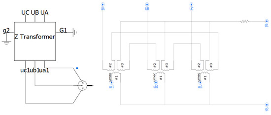
Figure 4.
External and internal simulation diagram of the grounding transformer.
2.3. Cable Model
According to the field data, the cable model of the wind farm consists of 35 kV copper core cross-linked polyethylene insulation, steel belt armor, and a polyethylene sheath power cable. The nominal cross-sectional area of the single-core conductor S is 400 mm2, the outer diameter of the cable is approximately 125.1 mm, the DC resistance of the cable wire is 0.047 Ω/km, and the minimum laying depth of the cable is set to 1 m [19]. The cable simulation model and various parameter settings are shown in Figure 5.
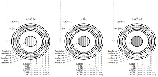
Figure 5.
Cable simulation model and various parameter settings.
3. Collection Line Fault Diagnosis Research Based on CNN-LSTM
During the operation of the wind farm, due to the influence of some natural and human factors, various faults and abnormal working conditions may occur in the cable line. Various phase-to-phase and ground short circuits may occur in cable lines due to conductor or insulation problems. The sheath current of the cable can better reflect these faults than the cable core current [20]. Therefore, this paper analyzes the characteristics of changes in the cable sheath current waveform, optimizes phase-mode transformation and neural network technology to achieve cable fault diagnosis, and uses traveling wave distance measurement theory and noise suppression methods to achieve cable fault location [21].
3.1. Improved Phase-Mode Transformation for Fault Classification
In the transmission line, the existence of electromagnetic coupling between phases leads to the non-diagonalization of the line parameter matrix, and the phase equations are interrelated. When the traveling wave propagation characteristics are directly analyzed or the fault equation is solved, the coupling effect becomes complicated. By selecting a specific matrix, the coupling parameter matrix is diagonalized to realize the decoupling of each mode component so that the complex multiphase problem is transformed into an independent single-mode problem [22].
The basic principle of phase-mode transformation is to transform the line parameter matrix in the coupled wave equation into a diagonal matrix by using the transformation matrix S and the transformation matrix Q, so that the original line equations are independent of each other. From the above analysis, it can be seen that the core of the phase-mode transformation is to select the mode transformation matrix S and Q. The commonly used phase-mode transformation matrices include symmetrical component transformation, Clarke transformation, and Karenbauer transformation. It is not possible to fully characterize all short-circuit fault types by using only one line mode component. In order to use the line mode component obtained by the traditional phase mode transformation method to characterize all short-circuit fault types, it is necessary to use both the line mode component and the line mode component , which brings a certain degree of inconvenience to the traveling wave fault location.
Therefore, an improved phase-mode transformation is proposed, making all short-circuit fault types able to be characterized by only a single line mode component. The following is the derivation process of the improved phase-mode transformation. Assuming that the three-phase transmission line is completely transposed, the line parameter matrix is set to P, where each element is shown as the following matrix, represents the self-impedance of the wire, and represents the mutual impedance between the wires:
Diagonalize the matrix P; let and the diagonal matrix , where the diagonal elements represent the eigenvalues of the parameter matrix P; and then let the characteristic equation , where E is the unit matrix, and the eigenvalue forms are as follows:
Let the eigenvectors corresponding to each eigenvalue be ,, and the subscript i = 1, 2, 3; then, the transformation matrix can be expressed as ; and then the following equations are obtained by using the relationship between eigenvalues and eigenvectors:
The relationship between the elements of the phase-mode transformation matrix can be obtained by the simultaneous equations:
The presence of zero-value elements in the inverse transformation matrix prevents the line-mode component from characterizing single-phase ground faults, while equal row elements cause failure in characterizing two-phase short-circuit ground faults. These inherent mathematical defects limit the applicability of traditional methods in complex fault scenarios. Hence, developing an improved phase-mode transformation matrix capable of characterizing all short-circuit fault types is essential.
By performing matrix transformation on the phasor signals of different fault types, linear mode components with clear physical meaning can be obtained. In particular, it is worth noting that no matter what form of short-circuit fault occurs on the line, there is always a specific current line-mode component after transformation that can accurately characterize the fault characteristics, as shown in Table 1.

Table 1.
Improved phase-mode transformation of different fault types.
3.2. Cable Fault Diagnosis Based on CNN-LSTM
Field operation experience shows that there are some faults with unobvious current signal characteristics and complex faults, which may lead to difficulties in conventional fault identification methods. It is necessary to use the experience of experts to complete the fault identification. Therefore, this paper introduces a CNN-LSTM hybrid neural network to realize intelligent identification of various possible complex fault types [23]. The neural network takes the electrical quantity time series data as input, the CNN layer extracts the local time-frequency and spatial distribution characteristics, the LSTM layer learns the time series dependence, and the output layer accurately determines the fault type through the Softmax classifier to provide prior information. It has a higher computational speed compared to other neural networks, better meeting the rapid fault classification requirements of relay protection during power line faults.
3.2.1. Convolutional Neural Network (CNN)
The convolutional layer of the convolutional neural network (CNN) contains multiple kernels. The 1D CNN provides inherent suitability for 1D time-series analysis (e.g., cable fault signals), as its kernels slide along the time axis, eliminating the need for signal-to-image conversion required by 2D CNNs. This avoids unnecessary data transformation and dimensionality expansion. The 1D CNN efficiently extracts local fault waveform features (transient mutations, wave heads) while preserving temporal dependencies. Figure 6 confirms its structural advantages: the CNN comprises input, output, and hidden layers, demonstrating superior computational efficiency and training speed for rapid cable fault diagnosis [24].
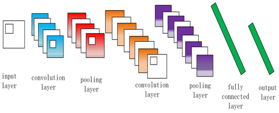
Figure 6.
Convolutional neural network structure diagram.
The CNN-LSTM model comprises a convolutional layer, a pooling layer, an LSTM layer, a fully connected layer, and a Softmax layer. To optimize its performance, comparative experiments were conducted on different channel numbers (16, 32, 64), revealing that the “32 + 64 channels” configuration is optimal: 32 channels effectively capture basic fault features, while 64 channels further extract detailed features, and no over-fitting occurs when trained on 700 groups of samples. Additionally, through comparative testing of learning rates (0.005, 0.01, 0.02), a learning rate of 0.01 was determined to yield the fastest convergence and the lowest loss. The specific parameters of the CNN-LSTM model structure are shown in Table 2.
Table 2.
CNN-LSTM model structure parameters.
3.2.2. Long Short-Term Neural Memory Network (LSTM)
Long short-term memory network (LSTM) is an improved recurrent neural network (RNN) variant that solves the gradient vanishing problem in long-sequence training through its gating mechanism. Its core comprises three gates (forgetting gate, input gate, output gate) and a cell state, dynamically regulating information flow: the forgetting gate filters obsolete information, the input gate updates new information, and the output gate controls current outputs [25]. Compared to traditional RNNs’ single-layer nonlinear transformations, this four-gated architecture demonstrates superior capability in capturing temporal features—including cross-period characteristics of power faults—and proves particularly suitable for long sequence-dependent scenarios, as illustrated in Figure 7.
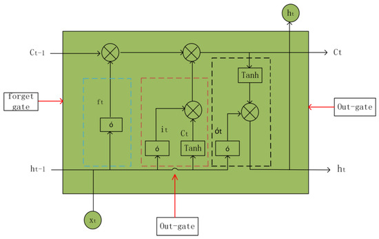
Figure 7.
LSTM unit structure diagram.
The LSTM achieves adaptive learning of sequential features through its forgetting gate, input gate, and output gate. This architecture eliminates redundant information, preserves essential features, and incorporates feature representations extracted by the CNN. The forgetting gate employs a sigmoid activation function to modulate the cell state, determining the retention degree of prior states. The input gate updates or stores new information based on activation values and candidate states. The output gate filters and transmits critical information according to the output activation and memory cell state. The specific calculation formula at time t is as follows:
where , , are the gate control calculation results; is the sigmoid activation function, and its output value is 0 or 1; the value of the Tanh activation function is between −1 and 1. ω is the weight matrix; W is the weight matrix of candidate values; h is the output of LSTM; U is the weight vector of the input state; is the input at time t; is the bias vector; is the memory unit state; and is a candidate state.
3.2.3. Cable Fault Diagnosis Model Analysis Based on CNN-LSTM
The CNN achieves automatic feature extraction via stacked convolutional layers, activation functions, and pooling layers. Its sliding-window convolution with weight sharing efficiently extracts signal features, while activation functions coupled with gradient descent accelerate convergence.
After using a convolutional neural network (CNN) to effectively extract the local time-frequency characteristics and spatial distribution of fault current signals, in order to further capture the dynamic time-series dependencies contained in the fault evolution process, especially the trend of fault transient signals over time and cross-period correlation characteristics, it is necessary to introduce a long short-term memory network (LSTM). With its unique gating mechanism, this network can effectively alleviate the problem of gradient disappearance when processing long sequence data so as to accurately learn the temporal evolution law of fault signals, form functional complementation with CNN, and jointly construct a complete fault diagnosis model.
The 3D feature tensor (including time step and multi-channel feature map) output from the last layer of CNN retains the temporal order of time steps by flattening or global pooling operations, merges the multi-channel features of each time step into feature vectors, and converts them into a 2D sequence of ‘time step × feature dimension’. After the sequence is directly input into LSTM, LSTM can further model long sequence dependencies across time steps (such as fault evolution law) based on local key features (such as fault transient mutations) captured by CNN so as to realize the joint modeling of local details and global temporal logic and avoid feature loss and redundant calculation [26].
The cable fault diagnosis process based on CNN-LSTM mainly includes data preprocessing, model training, and model evaluation. The main steps are as follows:
- (1)
- Using PSCAD to establish a typical wind farm model, set up various types of faults in the collector line system, obtain fault information, and collect on-site fault experience data and simulation data to form an original sample set.
- (2)
- The training set data is input into the CNN-LSTM model, and the convolution kernel is used to extract the fault feature, and the network parameters (such as batch size, learning rate, number of iterations, etc.) are repeatedly adjusted to optimize the model performance.
- (3)
- The maximum pooling operation is performed in the CNN part to retain the main features, and the all-0 filling is used to reduce the data dimension.
- (4)
- The pooled data is input into the double-layer LSTM network to train the neural network and learn the fault feature. Determine whether the current training number n reaches the set value M, and if not, continue training.
- (5)
- Complete the model evaluation.
- (6)
- Through the Softmax activation function, the fault diagnosis and classification are completed.
3.2.4. Simulation Study on Cable Fault Diagnosis Based on CNN-LSTM
To verify the effectiveness of the proposed method, this paper conducts a simulation study by establishing a fault diagnosis sample dataset with both simulation data and field-collected data. The dataset is split into 70% training samples (700 groups, with 70% being PSCAD simulation data and 30% actual wind farm measured data) and 30% test samples; a 1D convolution network is trained with the training samples through 700 iterations to obtain optimal parameters for cable fault classification, followed by validation using the test set to assess diagnostic accuracy. The CNN-LSTM hybrid framework has a total parameter size of approximately 500,000 (200,000 for the convolution layer and 300,000 for the LSTM layer), with a single sample processing time (including feature extraction and model reasoning) of about 20 ms, which meets the wind farm’s real-time requirement of a fault diagnosis response time under 100 ms.
The CNN-LSTM cable fault diagnosis process is shown in Figure 8:
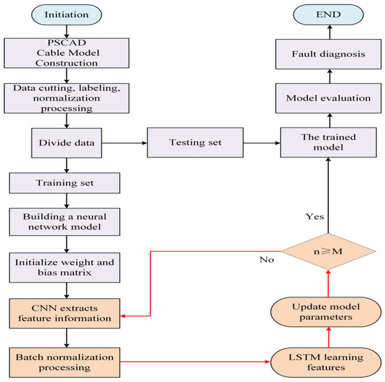
Figure 8.
CNN-LSTM fault diagnosis structure diagram.
The number of iterations and loss rate of the training set are shown in Figure 9, and the accuracy rate is shown in Figure 10.
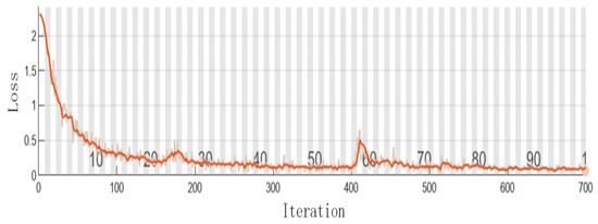
Figure 9.
Training loss value curve.
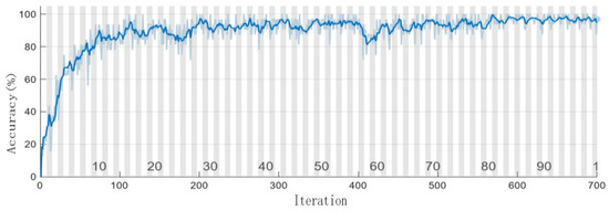
Figure 10.
Training accuracy curve.
The performance results of the training set and the test set are described in Figure 11 and Figure 12, respectively. Specifically, the training set reached 96.58% accuracy, while the test set reached 94% accuracy.
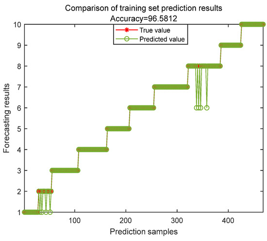
Figure 11.
Prediction results of the training set.
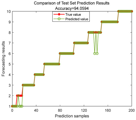
Figure 12.
Prediction results of the testing set.
The classification results of different faults are presented using the confusion matrix method. As illustrated in Figure 13 and Figure 14, the data in the right-hand column corresponds to the recall rate, while the data in the downward direction indicates the accuracy rate. The F1 score can be calculated based on these two metrics, and the resulting values align with the prediction outcomes.
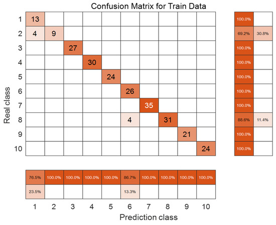
Figure 13.
Confusion matrix of the training set.
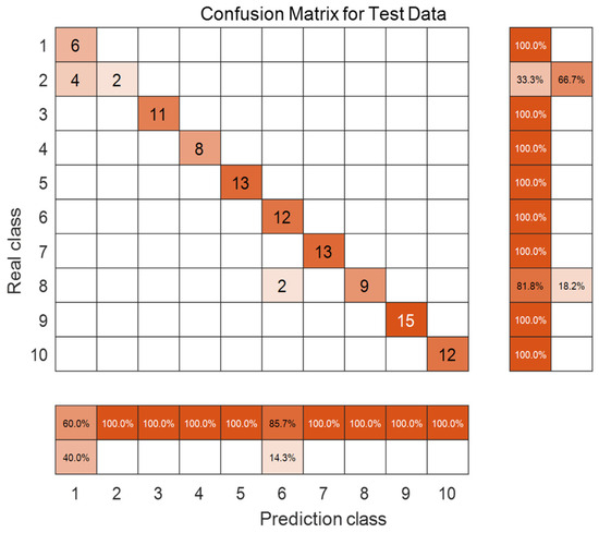
Figure 14.
Confusion matrix of the testing set.
From the above graphical data, it is evident that the CNN-LSTM model exhibits strong classification performance, enabling accurate identification of most faults. These include single-phase grounding faults, two-phase short-circuit faults, two-phase grounding short-circuit faults, and three-phase short-circuit faults. Nevertheless, for certain minor faults and complex faults with indistinct fault characteristics, the accuracy of fault diagnosis is somewhat lower. This is attributed to the insufficient accumulation of more expert experience data. However, the average recognition rate can still reach over 96.5%, indicating that the model has a favorable effect in determining fault types.
4. Fault Location Research of Collector Line Based on ICEEMDAN-PE-Improved Wavelet Threshold
4.1. Research on Double-Ended Fault Location of Collector Line Based on Improved Wavelet Transform
4.1.1. Improved Double-Ended Traveling Wave Ranging Method
In the cable line of a wind farm, because the conductor diameter and interval are small and the air is enclosed in the sheath, the traveling wave velocity of the cable is much slower than that of the overhead line, and it is difficult to measure due to the influence of environment and line aging, resulting in a large deviation between the theoretical and actual wave velocity. The optimized double-ended traveling wave ranging method is improved on the basis of the traditional double-ended traveling wave ranging method. Without the physical quantity of wave velocity, the fault location is calculated only by the time difference between the fault traveling wave and the measuring points at both ends so as to avoid the ranging error caused by the inaccurate wave velocity [27,28].
The calculation formula of fault location can be written as follows:
From the above simplification, it can be obtained:
where is the fault time from the fault point to the A end, is the fault time from the fault point to the B end, l is the full length of the line, d is the distance from the fault point to the A end, and v is the propagation speed of the fault traveling wave in the line.
4.1.2. Improved Wavelet Transform
Wavelet transform is a time-frequency analysis method that decomposes signals into different scales and positions using basis functions (wavelets). During decomposition, the original signal is decomposed layer by layer into high-frequency detail components (D) and low-frequency approximation components (A) via high-pass and low-pass filters [29]. Each decomposition stage halves the signal’s frequency range. The reconstruction phase synthesizes the original signal inversely. Mathematically, this decomposition-reconstruction mechanism is reversible, enabling extraction of local time-frequency characteristics from fault transient signals while ensuring complete information recovery. It has unique advantages in the fields of power system fault detection and signal denoising. The wavelet transform is defined as follows:
The wavelet transform is defined mathematically as follows:
where a represents the scale of a specific basis function, which is a scale parameter, and b represents the position of its translation along the x-axis, which is the time center parameter.
The selection of wavelet basis functions plays a critical role in signal processing and data analysis. Distinct characteristics of wavelet bases—including orthogonality, smoothness, and compact support—determine their suitability for different signal types and processing requirements. Through comparative analysis of Haar, Daubechies (db), Coiflets, Symlets, and Meyer wavelets, this study develops an improved wavelet transform method combining db20 with low-order db wavelets. This hybrid approach employs a strategic fusion of db20 and low-order db wavelets for harmonic signal processing. First, the high vanishing moment property of db20 enables precise frequency-band partitioning, effectively separating high-frequency and low-frequency components. Subsequently, based on low-frequency signal characteristics, a low-order db wavelet is selected to match the distortion points of the original signal for secondary processing. Its compact support characteristic suppresses decomposition distortion while reducing computational complexity to enhance real-time performance. This methodology forms complementary advantages by integrating the fine frequency division capability of high-order wavelets with the anti-distortion properties of low-order wavelets. It maintains time-frequency localization capabilities while offering engineering practicality, proving particularly effective for extracting detailed features from harmonic-rich complex signals [30].
The appropriate wavelet basis function and decomposition level are selected based on high-frequency signal characteristics. Given Daubechies wavelets’ superior orthogonality and compact support properties, the Db8 wavelet is chosen for decomposition. High-frequency cable signals exhibit a broad frequency range where energy distribution patterns become more distinct after 12 decomposition layers. Through 12-layer wavelet decomposition, cable high-frequency signals are separated into 13 frequency bands. The wavelet coefficients for each decomposition layer are then extracted, with their corresponding frequency band ranges detailed in Table 3.
Table 3.
Wavelet decomposition frequency range of each frequency band.
- (1)
- The time-domain signals of different frequency bands are reconstructed by inverse transform of the coefficients after wavelet decomposition.
- (2)
- According to the distribution characteristics of the frequency band, the 50 Hz component of the power frequency is mainly concentrated in the low frequency band corresponding to the A12 approximate component. Therefore, this frequency band can be selectively ignored when analyzing the high-frequency characteristics, and the signal components of the remaining 12 detailed frequency bands (D1–D12) are focused on.
- (3)
- The energy values of the reconstructed signals corresponding to 12 detail frequency bands (D1–D12) are calculated respectively, which are recorded as Ed1~Ed12. The energy is normalized: the sum of the energy of each frequency band E is calculated first, and then the ratio of the energy Edi of each frequency band to the total energy (Edi/E) is used as the characteristic quantity to characterize the energy distribution of the signal, that is, the input vector of fault diagnosis:
4.2. Research on Fault Denoising of Collector Line
The traveling wave fault location method has good accuracy in the noise-free ideal environment, but there are multi-source noises in the actual wind farm, such as telectromagnetic interference noise, line parameter variation noise, reflection and refraction noise, sampling noise, etc. Multi-source noise can affect the accuracy of selecting the peak value of the traveling wave head mode, making it difficult to precisely determine the position of the traveling wave front, which causes ranging errors [31,32].
4.2.1. Denoising Analysis Based on Permutation Entropy and Wavelet Threshold
Multi-source noise will greatly affect the accuracy of selecting modulus maxima after fault signal processing, resulting in large fault location calculation error. Therefore, a combined denoising method combining permutation entropy and threshold is proposed.
Permutation entropy (PE) is an index that quantifies the complexity by analyzing the local ordering pattern of time series. The core steps are as follows: (1) Set the embedding dimension (m) and time delay (τ), and reconstruct the original sequence into a multi-dimensional sub-vector; (2) the elements in each sub-vector are arranged in ascending order to generate a symbol sequence; and (3) count the probability of occurrence of each symbol sequence, calculate the information entropy based on the Shannon entropy formula, and normalize it to a value between 0 and 1. When the entropy value approaches 0, the sequence shows strong regularity; when it approaches 1, it is close to randomness. This method avoids the dependence on data distribution by extracting the inherent sorting features of the sequence and has the advantages of high computational efficiency and strong noise immunity, especially for the dynamic analysis of non-stationary and nonlinear systems.
The permutation entropy is defined as follows:
In order to make permutation entropy comparable, it is usually normalized:
where m is the embedding dimension.
Wavelet threshold denoising employed multi-resolution decomposition to expand signals into hierarchical structures, filtering transform-domain coefficients through threshold quantization to separate noise. The core methodology comprised two categories: static thresholds (preset parameters based on signal statistics) and dynamic thresholds (real-time adjustments driven by time-frequency features), respectively, embodying the design philosophies of predetermined rules and adaptive optimization.
The hard threshold function represents a direct denoising approach. When the absolute value of a wavelet coefficient exceeds or equals the predefined threshold, the coefficient is preserved unchanged. When the absolute value falls below this threshold, the coefficient is assigned zero. While this method effectively retains highly correlated signal components, it can induce discontinuities at threshold boundaries. The mathematical formulation is expressed as follows:
where is the wavelet coefficient of the original signal; is the wavelet coefficient after hard threshold processing; is the threshold.
The advantage of the hard threshold function is that it can effectively retain the characteristics of large amplitude signals, but its mutation processing mechanism produces discontinuity at the threshold, which is easy to cause pseudo-Gibbs phenomenon, resulting in distortion of reconstructed signals in visual quality and quantitative indicators.
The soft threshold function is relatively smooth. For the wavelet coefficient whose absolute value is greater than or equal to the threshold, shrink it to zero, that is, subtract the threshold; for wavelet coefficients whose absolute values are less than the threshold, they are also set to zero. Its mathematical expression is as follows:
where sgn is a sign function. The advantage of the soft threshold function is that it has continuity at the threshold, and the reconstructed signal is relatively smooth, and there is no discontinuity problem in the hard threshold function. However, soft threshold processing also brought some signal distortion. Because the coefficient larger than the threshold is shrunk, the amplitude of the signal will be reduced, and some details of the signal can be lost.
4.2.2. Analysis of Improved Wavelet Threshold Denoising Method
By analyzing the soft and hard threshold methods described in Section 4.2.1, it can be seen that both methods have defects. In order to solve the problems of soft and hard threshold methods, this paper improves the mathematical model of the threshold function, which is expressed as follows:
In the formula, the reference of each physical quantity is the same as that in the soft and hard threshold expressions, and the newly introduced is an improved threshold.
The expression is as follows:
In the formula, is the general threshold, and the formula represented the threshold of the k layer after wavelet decomposition.
The improved wavelet threshold has the following advantages:
- (1)
- solves the defect that the hard threshold function has discontinuity, strengthens the smoothness of the reconstructed signal, and also solves the disadvantage that the wavelet coefficient of the soft threshold function and the wavelet coefficient after denoising has fixed deviation.
- (2)
- The improved wavelet threshold function fused the hard/soft threshold characteristics by the adjustable parameter a: when a approaches 0, the hard threshold has a sharp cut-off, and a increases gradually, approaching the soft threshold continuous shrinkage. Simulation shows that when a = 1000, the balance between noise suppression and feature retention is optimal and the performance is the best.
4.2.3. Analysis of the ICEEMDAN Decomposition Algorithm
The adaptive noise complete ensemble empirical mode decomposition (ICEEMDAN) algorithm is optimized by dynamic noise control and multi-scale residual iteration: the white noise is not directly added to the original signal, but the noise is adjusted to the residual injection ratio according to the iteration stage, and the local mean denoising is extracted by the ensemble average method. The intrinsic mode function (IMF) is extracted step by step by using high-frequency to low-frequency hierarchical decomposition, and the residuals are updated to ensure completeness [33].
Compared with VMD (variational mode decomposition), although the VMD decomposition algorithm has strong anti-noise performance and can effectively avoid modal aliasing, it needs to set parameters such as modal number in advance, rely on empirical selection, and deal with boundary effects. Limited and vulnerable to interference components, as an adaptive decomposition method, ensemble empirical mode decomposition (EEMD) exhibits inherent limitations, including reconstruction errors and insufficient decomposition accuracy. Compared with EEMD and VMD, ICEEMDAN enhances modal component independence and signal reconstruction accuracy by means of adaptive noise injection and residual iteration [34].
The principle of the ICEEMDAN decomposition algorithm is shown in Figure 15:
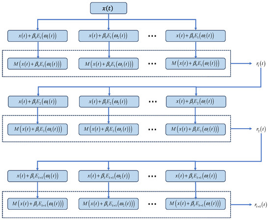
Figure 15.
ICEEMDAN decomposition algorithm schematic diagram.
The principle steps are as follows:
- (1)
- Firstly, white noise is added to the original signal to form a noisy signal :where is the white noise added for the ith time.
The signal is decomposed for the first time, the first-order component is taken, and then, the first IMF component is subtracted from the original signal to obtain the residual of the first stage:
The stator operator is the kth-order modal component obtained after EMD decomposition.
- (2)
- When k = 1, the first-order modal component is solved:
- (3)
- The second-order residual component is as follows:Thus, the second-order modal component is as follows:
- (4)
- Then the k-order residual component is as follows:
- (5)
- The k-order modal component is derived:
Repeat step (4) until the residual signal can no longer be decomposed.
4.2.4. ICEEMDAN-PE-Improved Wavelet Threshold Denoising Adaptive Algorithm
In this study, an adaptive algorithm based on ICEEMDAN-PE-improved wavelet threshold denoising was applied to process noisy signals from wind farm collector line faults [35]. The algorithm structure is illustrated in Figure 16.
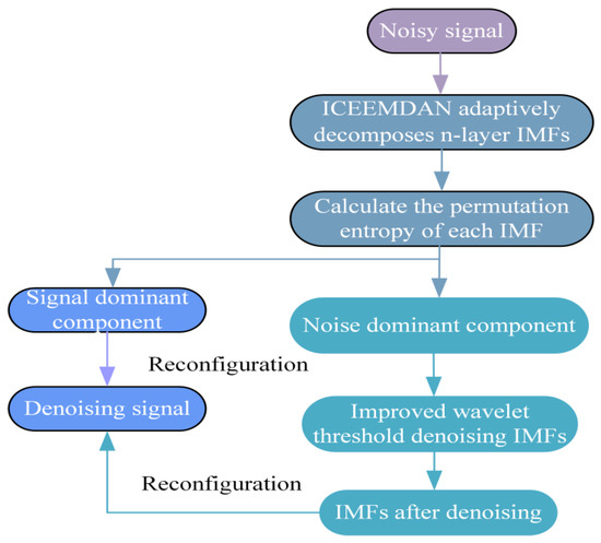
Figure 16.
ICEEMDAN-PE-wavelet threshold denoising algorithm structure diagram.
The principle of its adaptive denoising algorithm is as follows:
- (1)
- The signal containing noise is decomposed by ICEEMDAN, and the signal is decomposed into a series of modal functions (IMFs) and residual components.
- (2)
- During the decomposition process, each extracted IMF component undergoes local mean and residual calculation, followed by permutation entropy computation for every obtained modal component.
- (3)
- The permutation entropy threshold is determined, and each modal component is classified as signal-dominated or noise-dominated;
- (4)
- The noise-dominated IMF components are denoised by improved wavelet threshold denoising, and a set of noise-dominated denoised IMF components are obtained.
- (5)
- After all IMFs are classified and denoised, the denoised IMF components are reconstructed to obtain the final denoised signal.
Simulation results for the wind farm collector line appear in Figure 17, showing a decreasing trend in permutation entropy (PE) across successive IMF components. We tested PE thresholds of 0.6, 0.7, and 0.8: a threshold of 0.6 risks retaining excessive noise (as IMF components with PE close to 0.6 may still contain noise interference), while 0.8 can overly suppress useful signals (misclassifying IMF components with moderate randomness but containing fault features as noise). By setting the PE threshold to 0.7, which aligns with the natural transition between noise-dominated (PE ≥ 0.7 for early IMF components) and signal dominated (PE < 0.7 for later ones) in the simulation data, signal dominated components (PE < 0.7) are effectively distinguished. Compared with conventional methods, our improved wavelet threshold algorithm demonstrates precise noise component identification and targeted multi-scale processing. This approach avoids signal distortion while maintaining computational efficiency.
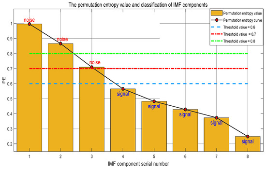
Figure 17.
The PE value of each modal component.
4.2.5. Simulation Analysis of Adaptive Algorithm Based on ICEEMDAN-PE-Improved Wavelet Threshold Denoising
Wind farms exhibit multi-source noise comprising mechanical interactions from rotating fan blades, bearing friction, and gear movements; structural resonance of generator towers under wind loads; and operational noise from electrical equipment. Guided by China’s Industrial Enterprise Boundary Environmental Noise Emission Standard [36] and Wind Farm Noise Limits and Measurement Methods [37], a measurement point on a hybrid collector branch was selected within the simulated wind farm collector system. Gaussian white noise was injected to replicate real-world wind farm noise conditions. The original signal with noise and the fault current signal with noise decomposed by ICEEMDAN-PE-improved wavelet threshold decomposition are shown in Figure 18. The first waveform is the original noisy signal, and the following seven waveforms are the signals of each layer of the original noisy signal after modal decomposition, which decrease layer by layer and finally tend to be gentle.
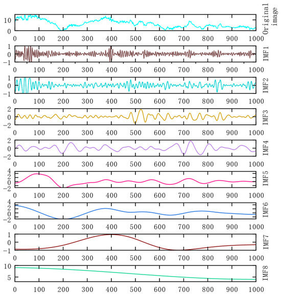
Figure 18.
ICEEMDAN-PE-improved wavelet threshold decomposition noisy fault current signal diagram.
In noisy signals, after denoising and reconstruction using ICEEMDAN-wavelet hard thresholding, ICEEMDAN-wavelet soft thresholding, and the ICEEMDAN-PE-improved wavelet threshold algorithm, the denoised results appear in Figure 19 and Figure 20. Figure 19 is the waveform comparison diagram of the original noisy signal and ICEEMDAN after three wavelet threshold processing. Figure 20 is the waveform comparison diagram of the original noisy signal and ICEEMDAN after three wavelet threshold denoising and reconstruction. It can be seen from the two diagrams that the waveform after ICEEMDAN improved wavelet threshold processing is smoother and the noise processing effect is better.
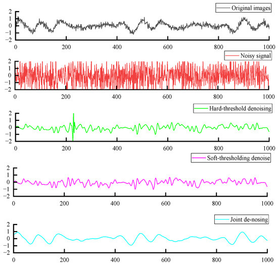
Figure 19.
ICEEMDAN-PE-improved wavelet threshold denoising image.
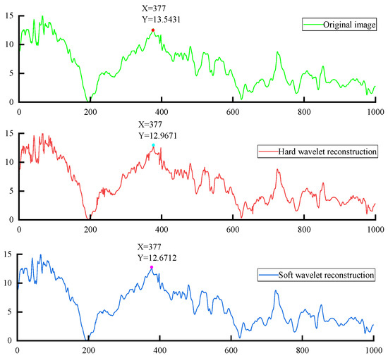
Figure 20.
ICEEMDAN-PE-improved wavelet threshold denoising reconstruction image.
To objectively evaluate reconstruction method performance and validate the proposed approach’s effectiveness, signal-to-noise ratio (SNR) and root mean square error (RMSE) were adopted as quantitative metrics. Five sets of fault current signals were collected under diverse collector line fault conditions. Following Gaussian white noise injection, three denoising methods were applied. Denoising efficacy was quantitatively assessed through SNR and RMSE calculations, with comparative results presented in Figure 21.
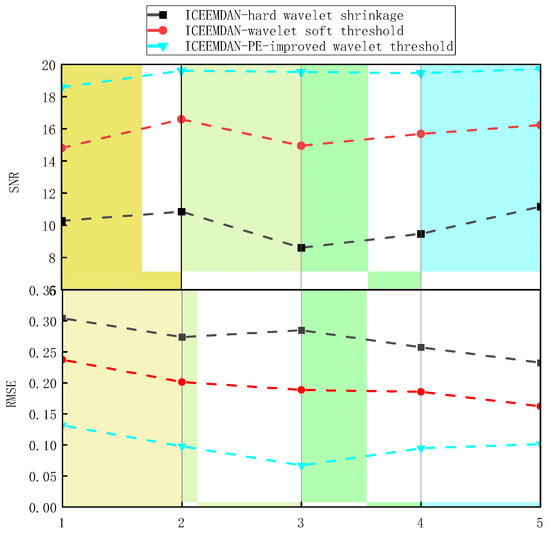
Figure 21.
SNR and RMSE evaluation index.
It can be seen that SNR > 18 dB and RMSE < 0.15 after ICEEMDAN-PE-improved wavelet threshold denoising. At the same time, this method is more stable than the other two methods for fault signal denoising under different fault conditions. Therefore, the method proposed in this paper has a significant effect on the denoising of the fault signal of the wind farm collector line, better retains the characteristics of the original signal, and improves the accuracy of the fault location of the collector line.
4.3. Research on Fault Location of Collector Line Based on Improved Wavelet Threshold
Pursuant to the proposed ICEEMDAN-PE-enhanced wavelet threshold denoising methodology, the denoised fault reconstruction signal was obtained and benchmarked against ICEEMDAN-wavelet hard thresholding (ICEEMDAN-WHT) and ICEEMDAN-wavelet soft thresholding (ICEEMDAN-WST). The enhanced wavelet algorithm, integrated with the modified double-ended traveling wave ranging method, was subsequently employed to simulate and analyze fault signals reconstructed through these distinct denoising approaches. To better compare and analyze the performance of the three proposed methods, the following assumptions were made during simulation:
- (1)
- When the system power supply is running normally, the three-phase voltage is strictly symmetrical.
- (2)
- Ignore the problem of asynchronous clocks at both ends during distance measurement.
- (3)
- The measurement errors, delays, and other influencing factors inherent in protective devices are also ignored.
4.3.1. Single-Phase Grounding Fault Diagnosis and Location Analysis Results of Different Denoising Methods
Five fault points are set on the collector line, including fault points F1, F2, F3, F4, and F5 near the end of the collector bus; fault points near the cable connection; part of the cable; and fault points near the end of the fan. For cables of different lengths, the fault points of F1 and F2 are set to 1000 m and 5000 m away from the collector bus in CABLE1, respectively. The fault points of F3 and F4 are set to 15,000 m and 24,000 m away from the collector bus in CABLE2, respectively. The fault point of F5 is set to 1000 m away from the collector bus in CABLE3, and the A-phase ground fault is set at each fault point to simulate the actual operating conditions on site. In the simulation, the short-distance cable adopts the ordinary model, and the long-distance cable adopts the cross-interconnection model [38]. The simulation result is shown in Table 4:
Table 4.
Single-phase grounding fault diagnosis and location analysis results.
4.3.2. Two-Phase Grounding Fault Diagnosis and Location Analysis Results of Different Denoising Methods
The same as the fault points set in the above Table 4, and the AC two-phase ground fault is set at each fault point. The simulation results are shown in Table 5:
Table 5.
Two-phase grounding fault diagnosis and location analysis results.
4.3.3. Two-Phase Short-Circuit Fault Diagnosis and Location Analysis Results of Different Denoising Methods
The same as the above fault point setting, and the BC interphase fault is set at each fault point. The simulation results are shown in Table 6:
Table 6.
Two-phase short circuit fault diagnosis and location analysis results.
4.3.4. Three-Phase Short-Circuit Fault Diagnosis and Location Analysis Results of Different Denoising Methods
The above fault point parameter setting is the same as the above, and three-phase short-circuit fault is set at each fault point. The simulation results are shown in Table 7:
Table 7.
Three-phase short circuit fault diagnosis and location analysis results.
Through the simulation and comparative study of the above Table 4, Table 5, Table 6 and Table 7, the following can be seen:
- (1)
- The reconstructed signal obtained by ICEEMDAN-PE-improved wavelet threshold denoising is more accurate than the reconstructed signal of the other two denoising methods through the fault location method used in this paper.
- (2)
- The fault location error near the terminal and cable connection will be too large, but the fault location accuracy of the denoising method in this paper is significantly improved compared with the other two denoising methods.
- (3)
- The results show that the ranging errors of different fault types are different. The single-phase grounding fault signal has strong asymmetry, uneven distribution of fault current, significant fluctuation of the zero-sequence component, and serious signal distortion, resulting in a larger calculation error of fault location than other faults. The three-phase short-circuit fault is a symmetrical fault. When the fault occurs, the signal amplitude is large and the anti-noise interference ability is strong. The signal feature extracted by wavelet transform is stable, so the calculation error of fault location is the smallest.
4.3.5. Fault Location Results of Transition Resistance with Different Resistance Values
In the power system fault, the single-phase ground fault accounts for the highest proportion, and the ranging error is large. The fault results show that when the transition resistance reaches 200 Ω, the calculation error of fault location of three different collector lines is significantly higher than that of low resistance fault. At the same time, the simulation study found that the signal distortion is not obvious when the high resistance fault occurs in different sections of the collector line, which increases the difficulty of fault location [39]. Therefore, to verify the effectiveness of the proposed fault location method under different levels of faults, this paper conducted simulation studies on single-phase grounding faults through transition resistance [40]. The three numerical transition resistances are used to represent the fault situation as follows:
- (1)
- 100 Ω indicates serious insulation damage, metal contact with the ground, poor contact with the equipment shell, etc.
- (2)
- 200 Ω indicates that the cable insulation is partially damaged or the overhead line contacts with high-resistance objects such as trees, forming incomplete grounding;
- (3)
- 500 Ω represents insulation damage, slight pollution, or leakage in a dry environment.
Set up five fault points at locations f1 = 500 m, f2 = 2000 m, f3 = 4000 m, f4 = 6000 m, and f5 = 8000 m away from the starting end of the cable line. Simulation results are shown in Table 8.
Table 8.
Simulation results of fault location through transition resistance grounding fault.
It can be seen from the table data that under the single-phase grounding fault of different transition resistances, the fault denoising and location method is minimally affected by the resistance value of the transition resistance for the cable line in the wind farm collector line and can effectively locate the fault point in various actual wind farm fault situations [41,42]. Especially for the common hybrid line fault location, the error caused by wave velocity instability, interference, and complex refraction and reflection of signals is overcome from the principle and algorithm. After calculation, the branch errors of the three collector lines are all within 0.5% of the total length, which meets the ranging accuracy and has good promotion value for studying various high-resistance fault conditions of wind farms.
5. Conclusions
Wind farm collector line faults have complex characteristics and are easily affected by noise signals. Especially during fault conditions involving transition resistance and complex faults, it is very difficult to effectively extract fault feature quantities. These issues pose severe challenges to traditional fault diagnosis and location methods. To resolve the problem of intelligent classification of various types of faults, the CNN-LSTM hybrid diagnosis model is constructed. The local time-frequency characteristics of the current signals are extracted by the CNN, and the dynamic time series law of the fault is captured by the LSTM. To achieve precise fault localization, an improved ICEEMDAN-PE wavelet threshold joint denoising algorithm is proposed. This method uses modal energy entropy to dynamically select effective traveling wave components, solving the problem of weakened wavehead characteristics in complex noise environments.
Based on the study of this paper, the following conclusions can be drawn.
- (1)
- Aiming at the problem of fuzzy characteristics of current signals under complex fault conditions, a hybrid model combining CNN and LSTM is proposed. CNN is responsible for extracting the local time-frequency characteristics of the current signal, and LSTM captures the dynamic time series law of the fault. The fault diagnosis method based on CNN-LSTM combined with phase-mode transform realizes the intelligent classification of various faults. The simulation results show that the fault diagnosis accuracy of the model is 96.5%, which effectively solves the limitations of traditional methods in feature extraction and complex fault classification.
- (2)
- Aiming at the problems of small fault current amplitude, low traveling wave amplitude, and easy disturbance by noise in high-resistance grounding fault, ICEEMDAN modal decomposition, permutation entropy (PE) threshold discrimination, and improved wavelet threshold technology are innovatively integrated. Through the collaborative optimization of modal decomposition and entropy threshold, the effective signal components are dynamically screened and the wavelet coefficients are optimized. In the simulation scenario injected with Gaussian white noise, the signal-to-noise ratio (SNR > 18 dB) is significantly improved and the root mean square error (RMSE < 0.15) is reduced, which provides a high-quality signal basis for subsequent fault location.
- (3)
- Taking the fault diagnosis results as a priori knowledge, the wave velocity and wavelet basis parameters in the two-terminal traveling wave ranging are adaptively calibrated. Combined with the signal reconstruction driven by noise reduction and the correction of the arrival time of the wave head, the fault location error is stably controlled within 0.5%. This method shows strong anti-interference in different fault types (such as single-phase grounding, two-phase short circuit, and three-phase short circuit), different transition resistances (100 Ω~500 Ω), and cable line scenarios, and it meets the engineering accuracy requirements.
However, this method has certain limitations in practical engineering applications. The dynamic changes of the system operation mode (such as load adjustment, power supply switching) will change the line parameters, affect the electrical characteristics of the positioning algorithm, and introduce errors. The inherent asymmetry of the power system (three-phase parameter difference, fault type asymmetry) will make the fault electrical signal more complex and interfere with the positioning logic; in the complex electromagnetic environment of the field, the disturbance, such as equipment start-stop and external radiation, is easy to pollute the monitoring signal, causing signal distortion and noise and reducing the positioning accuracy. In the future, the dynamic line parameter model can be constructed to adapt to the state change of the system, and the signal processing techniques, such as intelligent filtering and adaptive noise cancellation, can be introduced to weaken the interference.
Author Contributions
Conceptualization, H.D.; methodology, H.D. and S.B.; software, Z.G. and Y.Z.; validation, H.D. and S.B.; writing—original draft, H.D. and S.B.; writing—review and editing, Z.G. and Y.Z. All authors have read and agreed to the published version of the manuscript.
Funding
This research was supported by the Science and Technology Department Project of Jilin Province: Research on fault diagnosis and location of wind farm collector line based on situation awareness and deep learning algorithm. grant number 20240101101JC.
Data Availability Statement
Data are contained within the article.
Conflicts of Interest
The authors declare no conflicts of interest.
References
- Ding, Y. Green to new, new energy system to accelerate the construction of f new energy system. People’s Daily, 4 October 2024. [Google Scholar]
- Wu, Z.R.; Wu, J.T.; Li, Z.J. Fault diagnosis method of cable terminal grounding system based on metal sheath current and voltage. Electr. Technol. 2025, 145, 38–141. [Google Scholar] [CrossRef]
- Li, G.; Zhou, W.; Yu, Y.; Qiu, L.; Yang, B.; Ai, Y. Sheath current characteristics and fault diagnosis of adjacent common-ground high-voltage cable lines. High Volt. Eng. 2025, 51, 698–707. [Google Scholar] [CrossRef]
- Kok, C.L.; Ho, C.K.; Aung, T.H.; Koh, Y.Y.; Teo, T.H. Transfer Learning and Deep Neural Networks for Robust Intersubject Hand Movement Detection from EEG Signals. Appl. Sci. 2024, 14, 8091. [Google Scholar] [CrossRef]
- Kok, C.L.; Heng, J.B.; Koh, Y.Y.; Teo, T.H. Energy-, Cost-, and Resource-Efficient IoT Hazard Detection System with Adaptive Monitoring. Sensors 2025, 25, 1761. [Google Scholar] [CrossRef]
- Li, Z.H.; Cong, H. Power cable fault diagnosis based on chaotic systems and discrete wavelet transform convolutional neural networks. Autom. Appl. 2024, 65, 25–29. [Google Scholar] [CrossRef]
- Chi, P.; Liang, R.; Hao, C.; Li, G.; Xin, M. Cable fault diagnosis with generalization capability using incremental learning and deep convolutional neural network. Electr. Power Syst. Res. 2025, 241, 111304. [Google Scholar] [CrossRef]
- Ali, Y.M.; Ding, L.; Qin, S. An efficient approach for diagnosing faults in photovoltaic array using 1D-CNN and feature selection Techniques. Int. J. Electr. Power Energy Syst. 2025, 166, 110526. [Google Scholar] [CrossRef]
- Zhang, Y.H.; Zhou, T.T.; Huang, X.F.; Cao, L.C.; Zhou, Q. Fault diagnosis of rotating machinery based on recurrent neural networks. Measurement 2020, 167, 108774. [Google Scholar] [CrossRef]
- Sun, K.; Li, R.; Zhao, L.J.; Li, Z.Q. Feature extraction based on time-series topological analysis for the partial discharge pattern recognition of high-voltage power cables. Measurement 2023, 217, 113009. [Google Scholar] [CrossRef]
- Zhang, Y.L.; Xia, X.Y.; Xia, J.S.; Chen, S.Q.; Wang, R.Q.; Zhou, S. Fault diagnosis method of transmission cable based on Bagging-heterogeneous k-nearest neighbor. High Volt. Electr. Appar. 2023, 59, 104–112, 121. [Google Scholar] [CrossRef]
- Jiang, W.; Wang, D.; Hu, Y.; Liu, B.; Zhou, L.; Qian, G.; Li, Z. Fault Diagnosis for Shielded Cables Based on MSST Algorithm and Impedance Polar Plots. IEEE Trans. Instrum. Meas. 2024, 73, 3535212. [Google Scholar] [CrossRef]
- Shu, J.; Wang, Q.; Zhang, W.; Du, M.; Lin, J. Passive acoustic localization of submarine cable breakdowns using MUSIC algorithm combined with deep learning. Mar. Geophys. Res. 2025, 46, 5. [Google Scholar] [CrossRef]
- Li, Y.W. Analysis of fault diagnosis methods for power cables. Integr. Circuit Appl. 2025, 42, 372–374. [Google Scholar] [CrossRef]
- Kim, H.; Lee, H.; Kim, S.; Kim, S.W. Attention Recurrent Neural Network-Based Severity Estimation Method for Early-Stage Fault Diagnosis in Robot Harness Cable. Sensors 2023, 23, 5299. [Google Scholar] [CrossRef]
- Ding, C.; Chen, Y.; Nie, T. LVRT Control Strategy for Asymmetric Faults of DFIG Based on Improved MPCC Method. IEEE Access 2021, 9, 165207–165218. [Google Scholar] [CrossRef]
- NB/T 31026-2022; Electrical Design Specification for Wind Farm Engineering. Industry Standard of the People’s Republic of China: Beijing, China, 2022.
- DL/T 1631-2016; Relay Protection Configuration and Setting Technical Specifications of Grid-Connected Wind Farm. Industry Standard of the People’s Republic of China: Beijing, China, 2016.
- Jin, W.Q.; Wang, D.; Gao, H.L.; Peng, F.; Guo, Y.F.; Gao, M.Y.; Wang, J.W. Two-terminal traveling wave fault location approach based on frequency dependent electrical parameters of HVAC cable transmission lines. Electr. Power Syst. Res. 2024, 235, 110842. [Google Scholar] [CrossRef]
- Liu, F.; Xie, L.W.; Yu, K.; Wang, Y.P.; Zeng, X.J.; Bi, L.X.; Liu, F.; Tang, X. A novel fault location method based on traveling wave for multi-branch distribution network. Electr. Power Syst. Res. 2023, 224, 109753. [Google Scholar] [CrossRef]
- Liu, J.; Lee, C.K.; Pong, P.W.T. Online Short-Circuit Fault Diagnosis in Three-Core Power Distribution Cable Based on Magnetic Pattern. IEEE Sens. J. 2023, 23, 21832–21841. [Google Scholar] [CrossRef]
- Kim, H.; Jeong, H.; Lee, H.; Kim, S.W. Online and Offline Diagnosis of Motor Power Cables Based on 1D CNN and Periodic Burst Signal Injection. Sensors 2021, 21, 5936. [Google Scholar] [CrossRef]
- Huang, T.; Zhang, Q.; Tang, X.A.; Zhao, S.Y.; Lu, X.N. A novel fault diagnosis method based on CNN and LSTM and its application in fault diagnosis for complex systems. Artif. Intell. Rev. 2022, 55, 1289–1315. [Google Scholar] [CrossRef]
- Swaminathan, R.; Mishra, S.; Routray, A.; Swain, S.C. A CNN-LSTM-based fault classifier and locator for underground cables. Neural Comput. Appl. 2021, 33, 15293–15304. [Google Scholar] [CrossRef]
- Feng, R.; Du, H.; Du, T.; Wu, X.; Yu, H.; Zhang, K.; Huang, C.; Cao, L. Fault diagnosis for wind turbines based on LSTM and feature optimization strategies. Concurr. Comput. Pract. Exp. 2024, 36, e7886. [Google Scholar] [CrossRef]
- Chen, H.; Cen, J.; Yang, Z.; Si, W.; Cheng, H. Fault Diagnosis of the Dynamic Chemical Process Based on the Optimized CNN-LSTM Network. ACS Omega 2022, 7, 34389–34400. [Google Scholar] [CrossRef]
- Yang, S.; Li, T.; Pang, X.; Gu, C. A nondestructive high-resistance fault diagnosis method of XLPE medium voltage cables based on Chirp-TDR. Measurement 2024, 235, 115021. [Google Scholar] [CrossRef]
- Bonilla, L.M.; Orozco, H.R.A.; Cabrera, M.A. An overview of methods for detecting and locating incipient faults in underground cables. Electr. Power Syst. Res. 2025, 245, 111631. [Google Scholar] [CrossRef]
- Zhu, B.; Yu, X.; Tian, L.; Wei, X. Insulation Monitoring and Diagnosis of Faults in Cross-Bonded Cables Based on the Resistive Current and Sheath Current. IEEE Access 2022, 10, 46057–46066. [Google Scholar] [CrossRef]
- Jung, C.; Lee, J.; Wang, X.; Song, Y. Wavelet based noise cancellation technique for fault location on underground power cables. Electr. Power Syst. Res. 2007, 77, 1349–1362. [Google Scholar] [CrossRef]
- Parsi, M.; Crossley, P.; Dragotti, P.L.; Cole, D. Wavelet based fault location on power transmission lines using real-world travelling wave data. Electr. Power Syst. Res. 2020, 186, 106261. [Google Scholar] [CrossRef]
- Qi, Z.; Huang, Z.H.; Chen, Y.B. Impedance method based on zero-sequence component for fault location of distribution network. Power Syst. Prot. Control. 2023, 51, 54–62. [Google Scholar]
- Meng, Y.; Yang, Q.; Chen, S.; Wang, Q.; Li, X. Multi-branch AC arc fault detection based on ICEEMDAN and LightGBM algorithm. Electr. Power Syst. Res. 2023, 220, 109286. [Google Scholar] [CrossRef]
- Yu, D.; Zhou, N.; Liao, J.; Wang, Q.; Lyu, Y. Modified VMD Algorithm-Based Fault Location Method for Overhead-Cable Hybrid Transmission Line in MTDC System. IEEE Trans. Instrum. Meas. 2024, 73, 3517711. [Google Scholar] [CrossRef]
- Peng, L.; Guo, Z.; Zhang, S. Research on Fault Diagnosis Method of High-Speed EMU Air Compressor Based on ICEEMDAN and Wavelet Threshold Combined Noise Reduction. IEEE Access 2024, 12, 17348–17351. [Google Scholar] [CrossRef]
- GB 12348-2008; Industrial Enterprise Boundary Environmental Noise Emission Standard. National Standards of the People’s Republic of China: Beijing, China, 2008.
- DL/T 1084-2008; Noise Limit and Measurement Method of Wind Farm. Industry Standard of the People’s Republic of China: Beijing, China, 2008.
- Pan, X.; Zhao, D.; Chen, H.; Shen, A.; Wu, K. Incipient fault identification method for 10 kV power cables based on sheath current and DVAE-SAO-CatBoost. Electr. Power Syst. Res. 2025, 245, 111583. [Google Scholar] [CrossRef]
- Mo, S.; Zhang, D.; Li, Z.; Wan, Z. The Possibility of Fault Location in Cross-Bonded Cables by Broadband Impedance Spectroscopy. IEEE Trans. Dielectr. Electr. Insul. 2021, 28, 1418–1423. [Google Scholar] [CrossRef]
- Wang, C.; Zhao, X.; Qiao, J.; Xiao, Y.; Zhang, J.; Li, Y.; Cao, H.; Yang, L.; Liao, R. Structural Changes and Very-Low-Frequency Nonlinear Dielectric Response of XLPE Cable Insulation under Thermal Aging. Materials 2023, 16, 4388. [Google Scholar] [CrossRef]
- Wang, M.; Liu, Y.; Huang, Y.; Xin, Y.; Han, T.; Du, B. Defect Identification of XLPE Power Cable Using Harmonic Visualized Characteristics of Grounding Current. Appl. Sci. 2024, 13, 1159. [Google Scholar] [CrossRef]
- Xia, C.J.; Yang, M.J.; Chi, Z.B. A parameter-free fault location method for cross-bonding cable based on ranging equations. Electr. Power Syst. Res. 2024, 231, 110345. [Google Scholar] [CrossRef]
Disclaimer/Publisher’s Note: The statements, opinions and data contained in all publications are solely those of the individual author(s) and contributor(s) and not of MDPI and/or the editor(s). MDPI and/or the editor(s) disclaim responsibility for any injury to people or property resulting from any ideas, methods, instructions or products referred to in the content. |
© 2025 by the authors. Licensee MDPI, Basel, Switzerland. This article is an open access article distributed under the terms and conditions of the Creative Commons Attribution (CC BY) license (https://creativecommons.org/licenses/by/4.0/).