A Fault Direction Discrimination Method for a Two-Terminal Weakly Fed AC System Using the Time-Domain Fault Model for the Difference Discrimination of Composite Electrical Quantities

Abstract

The project of the flexible direct transmission of renewable energy has become an inevitable development trend for the large-scale grid connection of renewable energy. Its two-terminal weakly fed AC system is often composed of 100% power electronic equipment, which leads to an essential transformation in fault characteristics and protection requirements. At present, in research, the traditional directional elements are limited by the negative-sequence control strategy, resulting in the decline of their sensitivity and reliability. Therefore, this paper proposes a model for identifying directional elements using composite electrical quantities that is not affected by the control strategy of the two-terminal weakly fed AC system and can reliably identify the fault direction. Firstly, the adaptability of traditional directional elements under the negative-sequence current suppression strategy on both sides of the system when faults occur in the AC line was analyzed. Secondly, based on the idea of model recognition, the model relationship of fault voltage and current in the case of ground faults and non-ground faults occurring at different locations was analyzed. Finally, a fitted voltage was constructed and the Kendall correlation coefficient was introduced to achieve fault direction discrimination. Simulation results demonstrate that the proposed pilot protection scheme can operate reliably under conditions of 300 Ω transition resistance and 25 dB noise interference.

1. Introduction

In order to reduce the dependence on fossil energy and cope with the energy crisis and climate change challenges, China has always placed the development of clean energy in a strategic priority. According to the “14th Five-Year Plan for Renewable Energy Development” issued by the National Development and Reform Commission, it is expected that by 2030, China’s non-fossil energy consumption will reach about 25%. Among all kinds of renewable energy, solar energy has an important strategic position, and expanding the scale of photovoltaic power generation and improving utilization efficiency have become some of the core measures to promote the development of renewable energy in China [1]. At present, there are three main ways of large-scale grid-connected transmission of photovoltaic power stations: one is to integrate photovoltaic energy into the grid through AC transmission lines; another is the direct transmission of photovoltaic array power by traditional DC transmission; and the other is the use of modular multilevel converter–high voltage direct current (MMC-HVDC) technology for energy transmission. The regional distribution of energy resources in China is unbalanced, and there is a significant difference in energy distribution between the eastern and western regions. There is a large geographical distance between the main energy production base and the power consumption center. With the increasing capacity and transmission distance of renewable energy connected to the grid, the traditional AC transmission mode is facing certain challenges. Flexible HVDC has the advantages of a high output voltage quality, low harmonic content, low switching loss, large capacity, and high voltage transmission, and can also provide voltage support to passive power grid. Compared with traditional HVDC technology, flexible HVDC system has an active power independent regulation ability, which can realize flexible control of reactive power. At the same time, its topology effectively solves the commutation failure problem and has better adaptability and running performance. In general, flexible DC transmission technology can effectively solve the problem of the intermittent output of renewable energy, efficiently connect renewable energy to the power grid, improve the power grid’s absorption capacity of renewable energy, promote the optimization and construction of wide-area renewable energy, and become an ideal renewable energy transmission mode [2,3,4].

Renewable energy through the soft direct transmission project has become the inevitable development trend of large-scale renewable energy grid connection, and its two-terminal weakly fed AC system is often composed of 100% power electronic power equipment. Because the two-terminal weakly fed AC system contains a large number of power electronic devices, its current resistance is weak and the output fault current amplitude is limited and has variability, which requires that the protection device of the system have a fast and accurate fault identification ability and reliable operating characteristics to ensure the safe and stable operation of the system. As the first line of defense to ensure the safe and stable operation of the power system, the relay protection device of the power system must identify the fault accurately when the fault occurs on the outgoing line of the two-terminal weakly fed AC system so as to effectively prevent the fault expansion and maintain the reliable operation of the system. Among them, the directional element is not only the auxiliary element of distance protection but also the core element of directional comparison longitudinal protection, which plays an extremely important role in line protection. Its correct operation plays an important role in the safe and stable operation of the system. Therefore, it is necessary to study the directional elements suitable for a two-terminal weakly fed AC system.

While directional protection relays have been extensively studied, the current research primarily addresses AC lines in renewable energy systems connected directly to the grid. Limited attention has been given to AC line protection in flexible DC transmission systems where renewable stations interface with power electronic converters at both ends. Building upon a time-domain analysis, reference [5] developed a novel directional protection scheme utilizing waveform distance coefficients. This approach capitalizes on the distinct differences between the AC line current and boundary element current waveform characteristics during forward and reverse faults. However, the method’s effectiveness diminishes near DC terminal points due to measurement limitations. In reference [6], the maximum sensitivity angle is adaptively adjusted based on the parameters and operational state of the doubly fed fan, thereby enhancing the performance of conventional negative-sequence directional protection. However, this improved negative-sequence directional protection scheme still relies on traditional control strategies. Considering the fluctuating characteristics of positive-sequence impedance on the doubly fed induction generator (DFIG) side, reference [7] introduces a novel directional protection scheme based on amplitude variation differences in positive-sequence impedance. This approach leverages the distinct fault current behaviors between photovoltaic systems and synchronous generators. Based on the research on the differences in fault current characteristics between photovoltaic power generation system and synchronous generators, the literature [8] proposes a new principle for direction discrimination using fault current waveform distortion characteristics. However, the fault current difference between the two sides of the method is further weakened in the two-terminal weakly fed AC system, and its reliability needs to be further verified. The literature [9] proposes a fault direction identification method based on the combination criteria of voltage and current, which identifies the fault direction by analyzing the difference characteristics of positive- and negative-sequence current amplitudes in the case of forward and reverse faults. Reference [10] proposes a composite voltage–current criterion for fault direction identification, utilizing the amplitude disparity between positive- and negative-sequence currents during forward and reverse fault conditions. Reference [11] proposes a fault direction detection method that utilizes both the magnitude and phase characteristics of superimposed negative-sequence and positive-sequence impedances to identify fault directions for both symmetrical and asymmetrical faults. Reference [12] develops a directional protection scheme leveraging MMC control strategies. The method employs a controlled injection of a negative-sequence current to optimize the phase angle of negative-sequence impedance, thereby enabling a precise fault direction identification through a negative-sequence component analysis. Reference [13] redesigned the converter’s virtual fault component impedance characteristics through supplemental control strategy development. The study introduced distinct phase control methodologies for both virtual negative-sequence impedance and positive-sequence fault components, thereby enhancing the directional protection elements’ sensitivity and reliability. In the literature [14], the modulation circuit is used to compensate the distance of the AC transmission line to half of the power frequency wavelength, preventing the transmission of high-frequency signals. Based on the filtering characteristics, the high-frequency energy of the voltage signal is extracted by wavelet transform as the direction criterion. This method compensates the transmission line to the half-wavelength transmission line, but the line of the two-terminal weakly fed AC system is not more than a few hundred kilometers, and its adaptability in the two-terminal weakly fed AC system needs further study. Reference [15] enhances the operational performance of zero-sequence directional elements through impedance compensation techniques. However, this compensation scheme demonstrates applicability exclusively for ground fault scenarios, lacking generalizability to other fault types.

To sum up, domestic and foreign scholars have carried out a wide range of theoretical exploration and practical analyses of the fault characteristics of the renewable energy via AC system and research on the directional elements. When traditional directional elements are directly applied to the two-terminal weakly fed AC system, the following problems will exist:

(1)

The reliability problem of directional elements caused by the complexity of fault characteristics under the control strategy of the converter in the two-terminal weakly fed AC system is specifically manifested as described below. The different positive- and negative-sequence control strategies of the converters on both sides make the equivalent sequence impedance of the system show fluctuation characteristics different from those of the traditional synchronous machine, resulting in a reduction in the reliability of direction discrimination of the traditional directional elements.

(2)

The problem of fault identification sensitivity caused by the complexity of fault characteristics under the control strategy of the converter in the two-terminal weakly fed AC system is specifically manifested as the controlled characteristics of the converters on both sides weaken the characteristics of the output electrical quantity, resulting in a decrease in the sensitivity of fault direction discrimination of traditional directional elements.

(3)

The control functions of the line direction element and the converter in the two-terminal weakly fed AC system have not been fully integrated. Specifically, the vulnerability of the converter leads to the rapid entry of the converter into the fault control stage after a fault, causing the fault regulation time scale of the converter and the protection action time to tend to overlap. Changes in the fault characteristics will affect the action performance of the direction element.

A new direction discrimination method is proposed to overcome the influence that the traditional direction elements in the double-ended weakly fed AC system are controlled by the control strategy. An adaptive and highly reliable directional discrimination algorithm is proposed, aiming to establish an independent decision-making mechanism unaffected by control strategies and thereby achieving more dependable directional protection. This paper presents a time-domain fault model-based differential directional element using composite electrical quantities with the following key contributions:

(1)

This method avoids the influence of the control strategy when calculating the sequence impedance of traditional directional elements.

(2)

The idea based on model recognition only relies on identifying the relationship between fault voltage and current, and weak electrical quantities will not have an impact on this method.

(3)

This method can identify the fault direction by relying on the relationship between the fault electrical quantities in the fault control stage, and is not affected by the adjustment of the control strategy.

In this paper, a kind of directional element that is not affected by the control strategy is proposed for two-terminal weakly fed AC system under the background of a large-scale PV transmission project. Firstly, the sequence impedance characteristics of the two-terminal weakly fed AC system are analyzed, and then the adaptability of the traditional directional element is analyzed. Secondly, the relationship between voltage and current at the protection installation is analyzed. According to the fault phase, an electrical quantity of a forward ungrounded fault meets the positive resistance model, and the reverse ungrounded fault electrical quantity meets the negative resistance model. The zero-mode electrical quantity of the forward grounding fault meets the negative resistance model, and the zero-mode electrical quantity of the reverse grounding fault meets the positive resistance model. On this basis, the fitting voltage is constructed, the Kendall coefficient and average model error are introduced to reflect the relationship between the fitting voltage and the measured voltage, and the time-domain fault model differential discriminating direction element using the composite electrical volume is constructed. Finally, the PSCAD/EMTDC simulation platform is used to verify the performance of the directional element for different fault locations, fault types, transition resistances, photovoltaic outputs, noise influences, and different control strategies. The results show that the directional element can still operate reliably under the influence of 300 Ω and 25 dB noise transition resistance.

2. Adaptability Analysis of Traditional Directional Elements

The system topology and dual-control strategy of the photovoltaic (PV) power station with its booster and soft direct connection are illustrated in Figure 1. The PV station, with a capacity of 2000 MW, is first stepped up in voltage and then linked to the flexible direct converter station (MMC₁) via an AC line. From there, it connects to another converter station (MMC₂) through a DC line before being fed into the receiving grid. This study focuses on the 500 kV AC transmission line (MN) between the PV-side transformer and the flexible direct-side transformer. Among the fault points analyzed, f₁ and f₅ represent external faults, while f₂, f₃, and f₄ correspond to internal faults on the AC line.

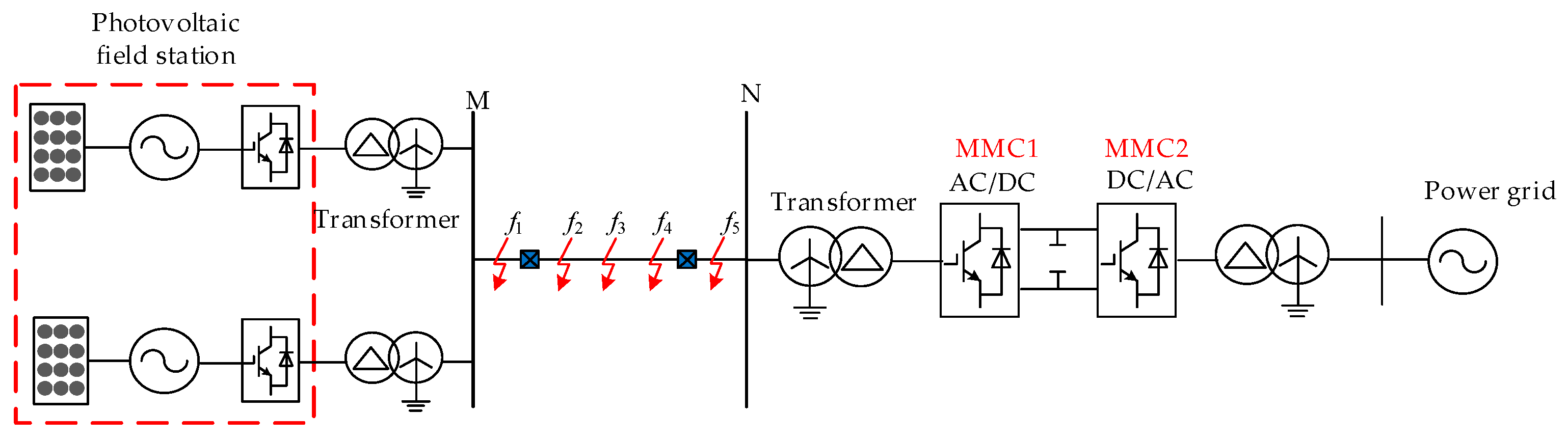
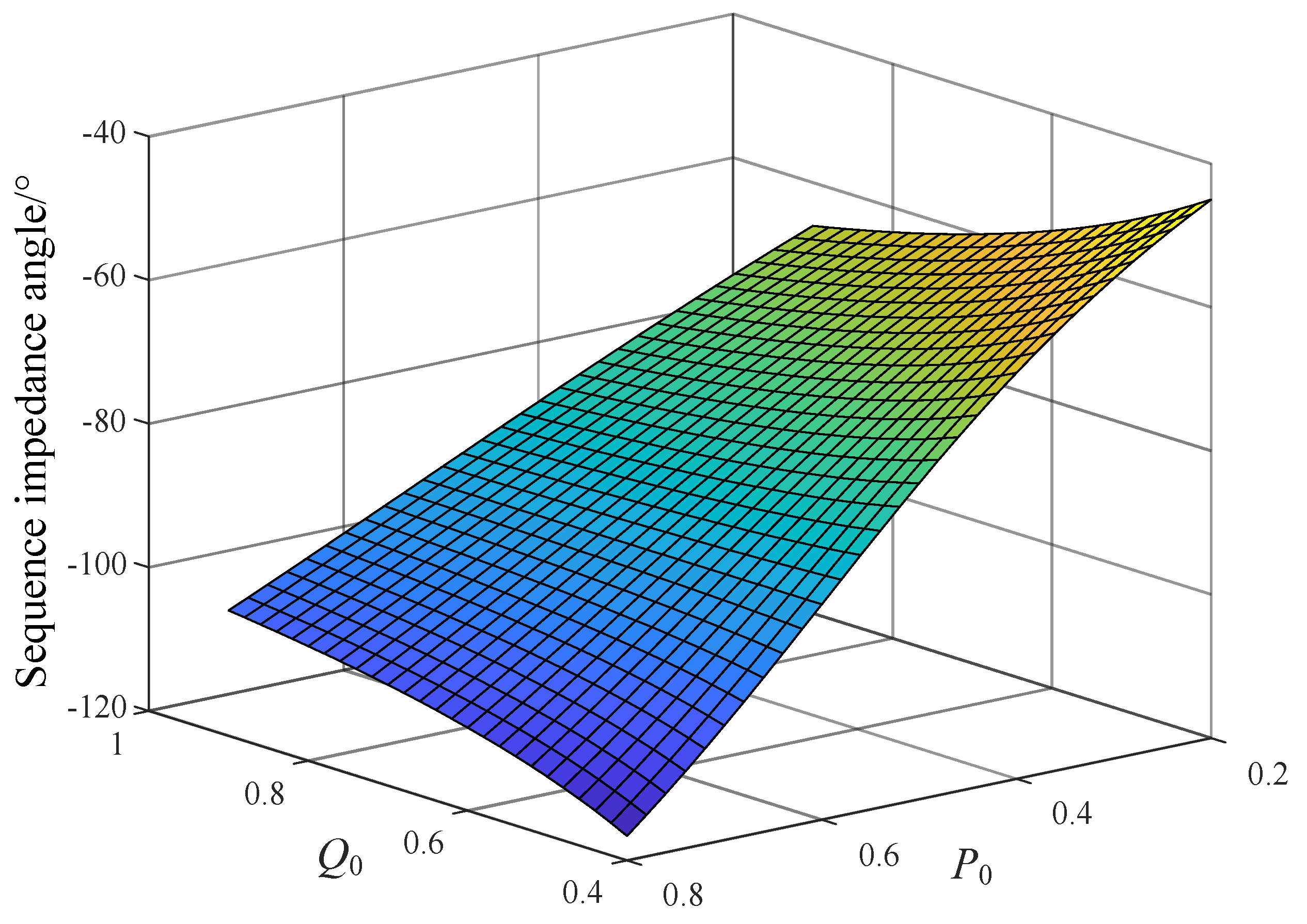
2.1. Analysis of the Sequence Impedance Characteristics of a Two-Terminal Weakly Fed AC System

Different from the traditional synchronous system, the two-terminal weakly fed AC system is affected by many factors, such as low voltage crossing measures, control strategies, and fault conditions during the fault period, and so it cannot be simply regarded as a linear system. Therefore, the equivalent impedance on both sides of the two-terminal weakly fed AC system has no practical physical significance and only represents the relationship between voltage and current at the protection installation. Firstly, the characteristics of positive sequence impedance on both sides are analyzed. Assume that the positive sequence voltage and current at both sides of the outlet before the fault is

$$\left\{\begin{array}{l}{U}_{x1}^{[0]}=U_{\mathrm{N}}\angle {\phi }_x\\ I_{x1}^{[0]}=I_{\mathrm{N}}\angle ({\phi }_0+{\phi }_x)\end{array}\right.,$$

(1)

where $U_{x1}^{[0]}$ and $I_{x1}^{[0]}$ are the positive-sequence voltage and current before the fault, and U_N and I_N are the amplitudes of rated voltage and rated current during normal operation. Based on the initial phase angle of voltage before the fault, φ₀ is the initial phase angle of the current. In normal operation, only active power is output on both sides of a two-terminal weakly fed AC system with the voltage and current in phase, giving φ₀ = 0°. x = A, B, C, representing the three phases A, B, and C, respectively, φ_A = 0°, φ_B = −120°, and φ_C = 120°.

In practical engineering implementations, accounting for both low-voltage ride-through requirements and the overcurrent limitations of power electronic switches, the output current of power electronic devices is typically constrained to within 1.2 times the rated current. Consequently, negative-sequence current suppression becomes the predominant control objective during fault conditions. For analysis purposes, we define the positive-sequence voltage and current outputs of the power electronic device during fault periods as follows:

$$\left\{\begin{array}{l}{U}_{x1}^{[0]}=U_{\mathrm{N}}\angle {\phi }_x\\ I_{x1}^{[0]}=I_{\mathrm{N}}\angle ({\phi }_0+{\phi }_x)\end{array}\right.,$$

(2)

where

$$\left\{\begin{array}{l}{I}_1={{\displaystyle \frac{1}{U}}}_1{I}_{\mathrm{N}}\angle ({\phi }_0+{\phi }_x)\\ \phi ={\tan }^{-1}{\displaystyle \frac{-Q_0}{P_0}}\end{array}\right.;$$

(3)

U₁ and I₁ are, respectively, the amplitudes of the forward sequence voltage and current after the fault; and P₀ and Q₀ are the reference values of active and reactive power, respectively. Δϕ is the positive sequence voltage transition angle. Substituting Equations (1) and (2) into the formula Z = ΔU_x1/ΔI_x1 for the equivalent positive sequence impedance in the sense of conventional protection algorithm, the following formula can be obtained:

$$Z_1={\displaystyle \frac{U_1(U_1(\cos \Delta \phi +\mathrm{j}\sin \Delta \phi )-U_{\mathrm{N}})}{P_0(\cos \Delta \phi +\mathrm{j}\sin \Delta \phi )+Q_0(\sin \Delta \phi -\mathrm{j}\cos \Delta \phi )-U_1{I}_{\mathrm{N}}}}.$$

(4)

The positive-sequence voltage jump angle Δφ is affected by the voltage drop and the impedance angle between the system and the line. Under certain fault conditions Δφ < 5°, it can be approximated that cosΔφ = 1 and sinΔφ = 0. Equation (4) can be simplified as follows:

$$Z_1={\displaystyle \frac{U_1(U_1-U_{\mathrm{N}})}{P_0-U_1{I}_{\mathrm{N}}-\mathrm{j}{Q}_0}}.$$

(5)

In the case of a positive-sequence voltage amplitude U₁ = 0.6 p.u., Figure 2 shows the phase angle of the positive-sequence impedance of both power sources in a two-terminal weakly fed AC system when the reference values of active and reactive power change. As evident from the graphical representation, the phase angle of the positive-sequence impedance exhibits a dynamic variation in response to changes in active and reactive power reference values, thereby precluding its characterization as a constant impedance parameter.

Since the control goal of the two-terminal weakly fed AC system during the fault is to suppress the negative-sequence current, ideally only the positive-sequence current is output; considering the noise and measurement errors in the signal sampling process, the protection element may not be able to measure the negative-sequence current reliably and accurately. Therefore, the phase angle of the negative-sequence impedance is uncertain. The phase angle of zero-sequence impedance fluctuates around 90° due to the influences of the transformer connection type and fault type.

2.2. Adaptive Analysis of Directional Elements of Traditional Sequence Components

The positive direction criterion of each sequence fault component direction element is shown as follows [16]:

• the positive-sequence fault component direction element is

  $$0°\le \arg {\displaystyle \frac{-\Delta {\dot{U}}_{\mathrm{m}1}}{\Delta {\dot{I}}_{\mathrm{m}1}}}\le 180°,$$

  (6)
• the negative-sequence direction element is

  $$0°\le \arg {\displaystyle \frac{-{\dot{U}}_{\mathrm{m}2}}{{\dot{I}}_{\mathrm{m}2}}}\le 180°,$$

  (7)
• and the zero-sequence directional element is

  $$0°\le \arg {\displaystyle \frac{-{\dot{U}}_{\mathrm{m}0}}{{\dot{I}}_{\mathrm{m}0}}}\le 180°.$$

  (8)

Among them, the positive-sequence fault component direction component is suitable for identifying the directions of all kinds of short-circuit faults, the negative-sequence component can be used for identifying the directions of asymmetric short-circuit faults, and the zero-sequence direction component is suitable for identifying the ground faults of asymmetric short-circuit faults. It can be seen that the application range of negative-sequence and zero-sequence directional components is more limited than that of positive-sequence fault component directional components.

Based on the analysis and conclusion of the sequence impedance characteristics of the two-terminal weakly fed AC system in Section 2.1, the adaptive analysis function is introduced, as shown in Equation (9):

$$\left\{\begin{array}{l}{x}^2+y^2=1\\ \theta =\arctan {\displaystyle \frac{y}{x}}\end{array}\right..$$

(9)

The positive-sequence impedance fluctuation angle and negative-sequence impedance fluctuation angle were substituted into the above equation and converted into a circle with radius of 1 and solved by MATLAB R 2018 b to obtain Figure 3. When a fault occurs, the relationship between the actual fluctuation region and the allowable fluctuation region of Z_M1 and Z_M2 is shown as the following figure, where the orange point is the actual possible fluctuation point of Z_M1 and Z_M2; the upper half circle is the correct operation area, that is, the allowed fluctuation area; and the lower half circle is the false operation area.

Figure 3 shows the mathematical transformation of the fluctuation range of the above-mentioned impedance phase angle into a circle with a radius of 1. The correct operating angle of the directional element is within the upper half of the circle, that is, 0 to 180°, and the incorrect operating angle of the directional element is within the lower half of the circle, that is, 0 to −180°. As the phase angle of the equivalent positive-sequence impedance on both sides of the two-terminal weakly fed AC system fluctuates greatly during the fault period, it will fall into the lower semicircle, that is, the misjudgment region, in Figure 3a. Therefore, when a fault occurs in front of the protection installation point on both sides, the directional component of the positive-sequence fault component has the problem of decreasing sensitivity and insufficient reliability in the two-terminal weakly fed AC system. Because the negative-sequence current suppression strategy is adopted on the photovoltaic side and MMC side of the two-terminal weakly fed AC system, there is no negative-sequence current in the outgoing line. In this case, the phase angle of the negative-sequence impedance on both sides of the two-terminal weakly fed AC system fluctuates randomly. In Figure 3b, it will fall into the lower semicircle, which is the error zone. The directional element based on the negative-sequence impedance component cannot identify the fault direction correctly. Since the impedance of the zero-sequence system on the back side of the protection installation is only related to the connection mode of the back-side transformer and the neutral point ground parameter, and has nothing to do with the characteristics of the power supply on the back side of the transformer, the phase of the line impedance and the system impedance can be approximately 90° for the zero-sequence network of a two-terminal weakly fed AC system. Therefore, the directional element based on the zero-sequence component can correctly identify the fault direction in the two-terminal weakly fed AC system. Therefore, it is necessary to propose an improved method of the traditional directional element that is not affected by the control strategy.

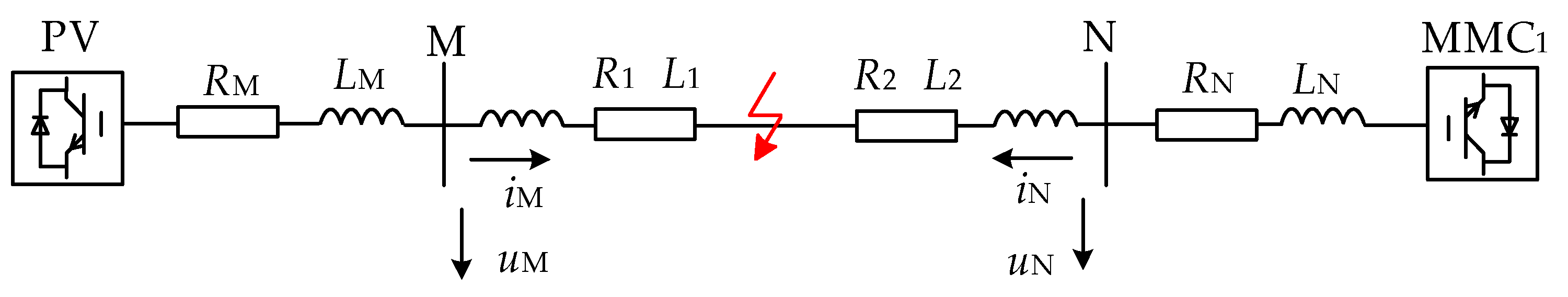
3. Model Difference Analysis

Aiming at the relatively stable characteristics of the zero-mode network of a two-terminal weakly fed AC system, the zero-mode component is selected to judge the direction of the ground fault, and the full components are selected to judge the direction of the non-ground fault. In addition, the directional element based on the zero-mode component can quickly identify the fault direction without matching with the phase selection element. Therefore, a time-domain fault model differential directional element based on the composite electrical volume is constructed.

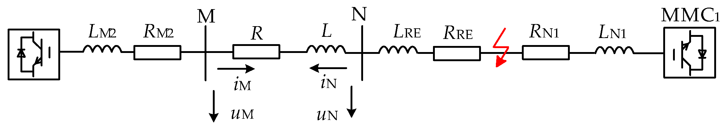
3.1. Zero-Mode Directional Element

The time-domain quantities can be converted to decoupled moduli by phase-mode transformation as transformed by Clark [17]:

$$\left[\begin{array}{l}{\mathrm{S}}_1\\ {\mathrm{S}}_2\\ {\mathrm{S}}_0\end{array}\right]=\left[\begin{array}{ccc}2& -1& -1\\ 0& \sqrt{3}& -\sqrt{3}\\ 1& 1& 1\end{array}\right]\left[\begin{array}{l}{\mathrm{S}}_{\mathrm{A}}\\ {\mathrm{S}}_{\mathrm{B}}\\ {\mathrm{S}}_{\mathrm{C}}\end{array}\right].$$

(10)

The zero-mode component voltage and zero-mode component current can be obtained as follows:

$$\left\{\begin{array}{l}{u}_0=(u_{\mathrm{A}}+u_{\mathrm{B}}+u_{\mathrm{C}})/3\\ i_0=(i_{\mathrm{A}}+i_{\mathrm{B}}+i_{\mathrm{C}})/3\end{array}\right..$$

(11)

Take the simulation model in Figure 1 as an example for a specific analysis. When a ground fault occurs at f₃, the directional element is a positive fault for both protection installations. Figure 4 shows the zero-mode network model. For the sake of generality, the fault of grounding through transition resistance is analyzed as an example.

In the figure, i_{M_0}, i_{N_0}, u_{M_0}, and u_{N_0} are the zero-mode current and zero-mode voltage measured at the protection installation points on both sides, respectively. R_{M_0}, L_{M_0}, R_{N_0}, and L_{N_0} are the zero-mode equivalent resistance and zero-mode equivalent inductance from the protection installation point to the neutral point of the system on the back side, respectively. R_{1_0}, L_{1_0}, R_{2_0}, and L_{2_0} are the zero mode equivalent resistance and zero mode equivalent inductance, respectively. R_f is the transition resistance value of the ground point; i_{f_0} is the zero-mode current flowing into the fault point.

As shown in Figure 4, in the zero-mode network model, the zero-mode voltage at the protection installation and the zero-mode current flowing through the network meet the following requirements:

$$\left\{\begin{array}{l}{u}_{\mathrm{M}\_0}=-R_{1\_0}{i}_{\mathrm{M}\_0}-L_{1\_0}{\displaystyle \frac{d{i}_{\mathrm{M}\_0}}{dt}}\\ u_{\mathrm{N}\_0}=-R_{2\_0}{i}_{\mathrm{N}\_0}-L_{2\_0}{\displaystyle \frac{{di}_{\mathrm{N}\_0}}{dt}}\end{array}\right..$$

(12)

According to Formula (12), when the ground fault occurs in the positive direction of the directional element, the fault model that meets the zero-mode current and zero-mode voltage measured at the protection installation is the series model of negative resistance and negative inductance, as shown in Figure 5.

When a ground fault occurs at f₅, the directional component is faulty in the positive direction for the photovoltaic side and in the reverse direction for the MMC side. Figure 6 shows the zero-mode network model.

As shown in Figure 6, in the zero-mode network model, the zero-mode voltage at the protection installation and the zero-mode current flowing through the network meet the following requirements:

$$\left\{\begin{array}{l}{u}_{\mathrm{M}\_0}=-R_{\_0}{i}_{\mathrm{M}\_0}-L_{\_0}{\displaystyle \frac{d{i}_{\mathrm{M}\_0}}{dt}}\\ u_{\mathrm{N}\_0}=(R_{\_0}+R_{\mathrm{M}\_0})i_{\mathrm{N}\_0}+(L_{\_0}+L_{\mathrm{M}\_0}){\displaystyle \frac{{di}_{\mathrm{N}\_0}}{dt}}\end{array}\right..$$

(13)

As can be seen in Formula (13), when the ground fault occurs in the positive direction of the directional element, the fault model of the zero-mode current and zero-mode voltage measured at the protection installation satisfies the series model of negative resistance and negative inductance; when the ground fault occurs in the opposite direction of the directional element, the zero-mode current and zero-mode voltage measured at the protection installation satisfy the positive resistance and positive inductance model, as shown in Figure 7.

When a ground fault occurs at f₁, the directional component is faulty in the reverse direction for the PV side and in the positive direction for the MMC side. Figure 8 shows the zero-mode network model.

As shown in Figure 8, in the zero-mode network model, the zero-mode voltage at the protection installation point and the zero-mode current flowing through the network meet the following requirements:

$$\left\{\begin{array}{l}{u}_{\mathrm{M}\_0}=(R_{\_0}+R_{\mathrm{N}\_0})i_{\mathrm{M}\_0}+(L_{\_0}+L_{\mathrm{N}\_0}){\displaystyle \frac{d{i}_{\mathrm{M}\_0}}{dt}}\\ u_{\mathrm{N}\_0}=-R_{\_0}{i}_{\mathrm{N}\_0}-L_{\_0}{\displaystyle \frac{{di}_{\mathrm{N}\_0}}{dt}}\end{array}\right..$$

(14)

As can be seen in Formula (14), when the ground fault occurs in the positive direction of the directional element, the fault model of the zero-mode current and zero-mode voltage measured at the protection installation satisfies the series model of negative resistance and negative inductance; when the ground fault occurs in the opposite direction of the directional element, the zero-mode current and zero-mode voltage measured at the protection installation satisfy the positive resistance and positive inductance model, as shown in Figure 9.

In summary, when a ground fault occurs on the output line of a two-terminal weakly fed AC system, if the fault occurs in the positive direction of the directional element, the model of the zero-mode current and zero-mode voltage at the protection installation is the series model of negative resistance and negative inductance. Otherwise, the model where the zero-mode current and zero-mode voltage at the protection installation meet is the series model of positive resistance and positive inductance.

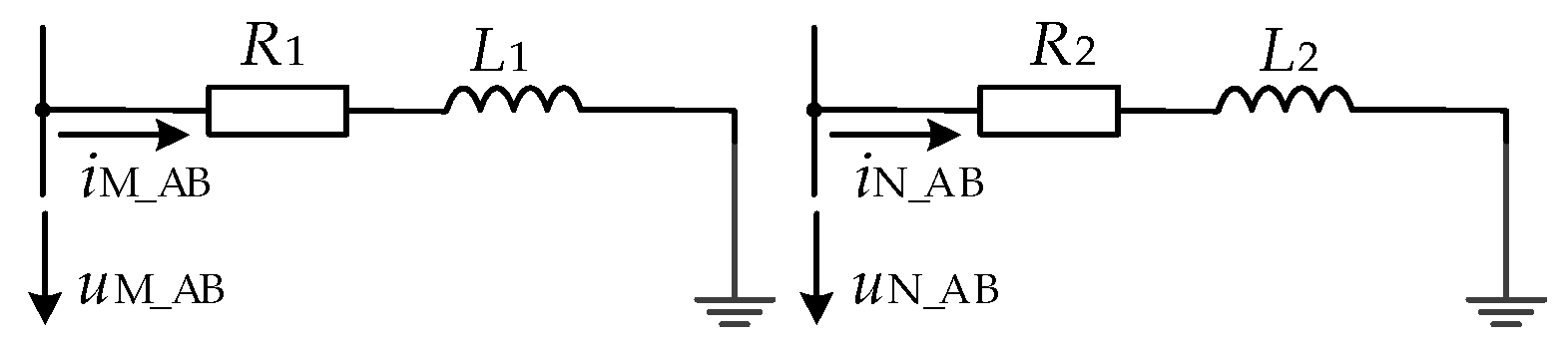
3.2. Full Directional Elements

When an ungrounded fault occurs in the outgoing line of a two-terminal weakly fed AC system, it is recommended to use the full identification of the fault direction relative to the protection installation point. In order to make the full directional elements correctly judge the direction of various fault types, the fault phase is first selected by the phase selection element, and u and i are determined.

The AB phase fault in the simulation model in Figure 1 is taken as an example for analysis. When an AB phase fault occurs at f₁, the directional element is a fault in the backward fault for the photovoltaic side and a fault in the positive direction for the MMC side. For the convenience of analysis, a single-phase equivalent model is presented in Figure 10.

In the figure, R_RE and L_RE are the equivalent resistance and equivalent inductance from the reverse fault point to the protection installation point, respectively. Convert the single-phase equivalent model in Figure 10 into a specific phase, and the fault-phase voltage and current flowing at the protection installation site meet the following requirements:

$$\left\{\begin{array}{l}{u}_{\mathrm{M}\_\mathrm{AB}}=-R_{\mathrm{RE}}{i}_{\mathrm{M}\_\mathrm{AB}}-L_{\mathrm{RE}}{\displaystyle \frac{{di}_{\mathrm{M}\_\mathrm{AB}}}{dt}}\\ u_{\mathrm{N}\_\mathrm{AB}}=(R+R_{\mathrm{RE}})i_{\mathrm{N}\_\mathrm{AB}}+(L+L_{\mathrm{RE}}){\displaystyle \frac{d{i}_{\mathrm{N}\_\mathrm{AB}}}{dt}}\end{array}\right..$$

(15)

As can be seen in Formula (15), when the interphase fault occurs in the positive direction of the directional element, the fault model measured at the protection installation site meets the series model of positive resistance and positive inductance. When the interphase fault occurs in the opposite direction of the directional element, the fault model is as follows: the fault phase voltage measured at the protection installation and the current flowing through the phase meet the negative resistance and negative inductance models, as shown in Figure 11.

Figure 12 shows the single-phase equivalent network model when the directional component is positive to the protection installation points on both sides when the fault occurs at f₃.

Convert the single-phase equivalent model in Figure 12 into a specific phase, and the fault-phase voltage and current flowing at the protection installation site meet the following requirements:

$$\left\{\begin{array}{l}{u}_{\mathrm{M}\_\mathrm{AB}}=R_1{i}_{\mathrm{M}\_\mathrm{AB}}+L_1{\displaystyle \frac{d{i}_{\mathrm{M}\_\mathrm{AB}}}{dt}}\\ u_{\mathrm{N}\_\mathrm{AB}}=R_2{i}_{\mathrm{N}\_\mathrm{AB}}+L_2{\displaystyle \frac{d{i}_{\mathrm{N}\_\mathrm{AB}}}{dt}}\end{array}\right..$$

(16)

It can be seen in Formula (16) that when the interphase fault occurs in the positive direction of the directional element, the fault model met by the fault phase voltage measured at the protection installation and the current flowing through the phase is the series model of positive resistance and positive inductance, as shown in Figure 13.

When a fault occurs at f₅, the directional element is a positive fault on the photovoltaic side and a reverse fault on the MMC side. A single-phase equivalent model is presented for the ease of analysis in Figure 14.

Convert the single-phase equivalent model in Figure 14 into a specific phase, and the fault-phase voltage and current flowing at the protection installation site meet the following requirements:

$$\left\{\begin{array}{l}{u}_{\mathrm{M}\_\mathrm{AB}}=(R+R_{\mathrm{RE}})i_{\mathrm{M}\_\mathrm{AB}}+(L+L_{\mathrm{RE}}){\displaystyle \frac{d{i}_{\mathrm{M}\_\mathrm{AB}}}{dt}}\\ u_{\mathrm{N}\_\mathrm{AB}}=-R_{\mathrm{RE}}{i}_{\mathrm{N}\_\mathrm{AB}}-L_{\mathrm{RE}}{\displaystyle \frac{d{i}_{\mathrm{N}\_\mathrm{AB}}}{dt}}\end{array}\right..$$

(17)

As can be seen in Formula (17), when the interphase fault occurs in the positive direction of the directional element, the fault model measured at the protection installation site meets the series model of positive resistance and positive inductance. When the interphase fault occurs in the opposite direction of the directional element, the fault model is as follows: the fault phase voltage measured at the protection installation and the current flowing through the phase meet the negative resistance and negative inductance models, as shown in Figure 15.

In summary, when an ungrounded fault occurs on the outgoing line of a two-terminal weakly fed AC system, if the fault occurs in the positive direction of the directional element, the model of the phase-to-phase current and phase-to-phase voltage of the fault phase meets the series model of positive resistance and positive inductance. If the fault occurs in the opposite direction of the directional element, the model of the fault phase’s interphase current and interphase voltage is the series model of negative resistance and negative inductance. In the above analysis, only the line model is identified, without any restriction on the power supply, that is, it is not affected by the fault characteristics of the power supply. Therefore, based on the idea of model recognition, the subsequent direction element that is not affected by the control strategy is proposed.

3.3. Feature Extraction

(1)

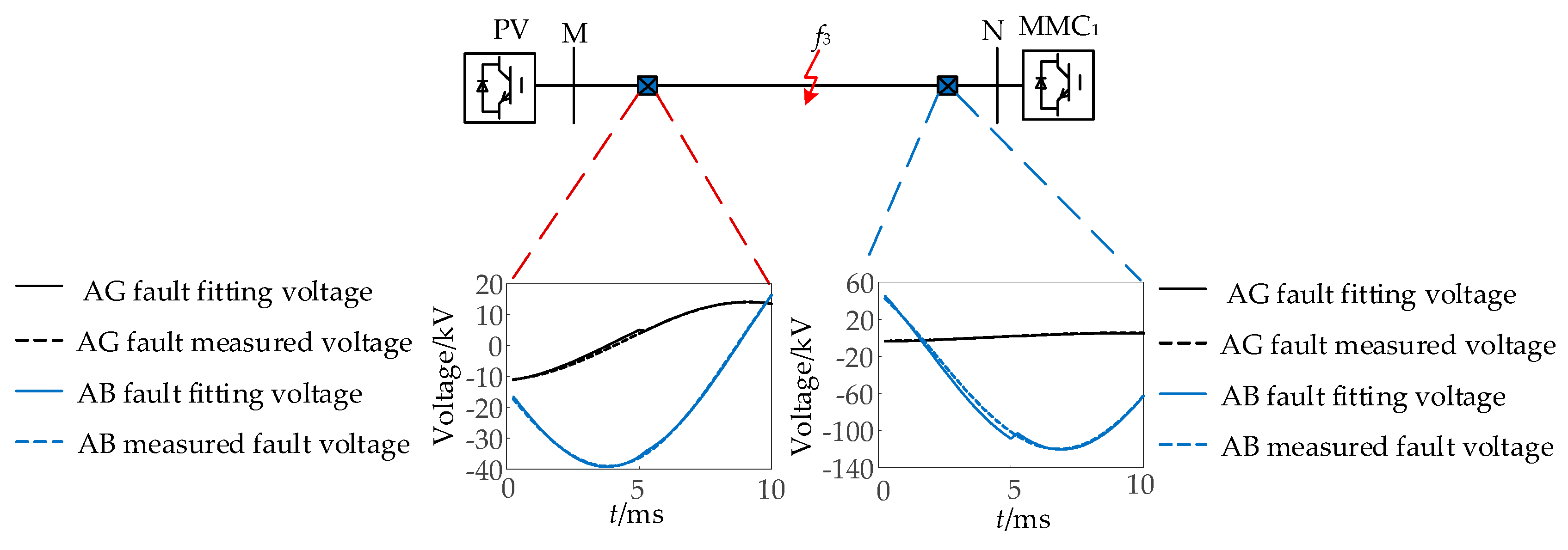
The introduction of fitted voltage and measured voltage

Based on the differences in the forward and forward direction models, forward fault fitting voltage and measured voltage are introduced in this section, which lay a foundation for identifying the fault direction using the relationship between the fitted voltage and measured voltage. The forward fault fitting voltage definition is similar for grounded faults and ungrounded faults.

When a fault occurs on the output line of a two-terminal weakly fed AC system, assuming that the short-circuit fault occurs in the positive direction of the protection installation, the forward equivalent resistance R* and equivalent inductance L* from the fault point to the protection installation point can be calculated by the idea of parameter recognition. Then the forward fault fitting voltage u_ft can be constructed using the forward equivalent parameters. At the same time, remember that the measured voltage at the protection installation is u_at.

(2)

Characteristic difference analysis of the fitted voltage and measured voltage in the positive and negative directions

This section uses a grounding fault at the protection installation point of the photovoltaic side as an example. In the fault simulation model shown in Figure 1, when f₃ fails, that is, when the fault is in the positive direction relative to the light-voltage side protection installation, the fitting zero-mode voltage u_ft can be calculated as follows:

$$u_{\mathrm{ft}}=-R^{*}{i}_{\mathrm{M}\_0}-L^{*}{\displaystyle \frac{d{i}_{\mathrm{M}\_0}}{dt}},$$

(18)

where −R* and −L* are, respectively, the positive equivalent zero-mode resistance and equivalent zero-mode inductance calculated from the protection installation point to the fault point using the parameter identification algorithm assuming that the grounding fault occurs in the positive direction; u_ft is the forward fault fitting voltage. At this time, the measured zero-mode voltage at the PV side protection installation is u_at, and the measured value of u_at is shown in Formula (12). At this time, both u_at and u_ft are negative resistance models. In the time-domain waveform, u_at and u_ft show the same direction and almost the same size. When constructing the above forward fitting voltage, the difference between a grounded fault and a non-grounded fault is that the fitting voltage u_ft of a non-grounded fault due to polarity is

$$u_{\mathrm{ft}}=R^{*}{i}_{\mathrm{M}\varphi \varphi }+L^{*}{\displaystyle \frac{d{i}_{\mathrm{M}\varphi \varphi }}{dt}},$$

(19)

When ground faults and non-ground faults occur at different locations in the simulation model, as shown in Figure 1, the relationship between the fitted voltage and the measured voltage obtained through the above analysis and calculation is shown in Figure 16, Figure 17 and Figure 18. As shown in Figure 16, Figure 17 and Figure 18, when faults occur at different locations, the fitting voltage is the same as the measured voltage when the fault is in the positive direction, while the fitting voltage is the same as the measured voltage when the fault is in the opposite direction, which is consistent with the theoretical analysis mentioned above.

4. Fault Direction Discrimination Method Based on Model Recognition

4.1. The Introduction of the Kendall Coefficient

A correlation analysis is a statistical method used to study the relationship between random variables, aiming to explore whether there is a certain dependence between variables and further analyze the direction and degree of correlation of variables that have a dependence relationship, including linear correlation analysis, partial correlation analysis and distance correlation analysis. Among them, linear correlation analysis is often used to study the degree of linear dependence between variables [18]. Among them, there are many methods to calculate waveform correlations [19,20], such as cosine similarity, Pearson’s correlation coefficient, Spearman’s correlation coefficient, generalized Jacquard coefficient, the Kendall correlation coefficient, etc. The Kendall correlation coefficient is a statistical index used to measure the consistency or correlation between two groups of data, and its value range is [−1, 1], where −1 means a completely negative correlation, 1 means a completely positive correlation, 0 means no correlation, and its calculation result is expressed by the correlation coefficient τ.

The discretized fitting voltage and measured voltage in the time domain are shown as follows:

$$\left\{\begin{array}{l}{u}_{\mathrm{at}}=\left\{u_{\mathrm{at}1},u_{\mathrm{at}2},u_{\mathrm{at}3},\cdots ,u_{\mathrm{at}x}\right\}\\ u_{\mathrm{f}\mathrm{t}}=\left\{u_{\mathrm{ft}1},u_{\mathrm{ft}2},u_{\mathrm{ft}3},\cdots ,u_{\mathrm{ft}x}\right\}\end{array}\right.,$$

(20)

where x is the number of sampling points.

The discretized voltage fitting voltage and actual voltage data in the time domain are put into the set shown in the following formula:

$$\mathrm{u}=\left.\left\{(u_{\mathrm{at}1},u_{\mathrm{ft}1}),(u_{\mathrm{at}2},u_{\mathrm{ft}2}),(u_{\mathrm{at}3},u_{\mathrm{ft}3}),\dots ,(u_{\mathrm{at}x},\right.u_{\mathrm{ft}x})\right\}.$$

(21)

The Kendall correlation coefficient is calculated as follows:

$$\tau ={\displaystyle \frac{n_c-n_d}{\sqrt{(n_0-n_1)(n_0-n_2)}}},$$

(22)

where τ is the calculated Kendall correlation coefficient; nc is the logarithm of elements satisfying consistency in set u; nd is the logarithm of elements in set u that do not satisfy the consistency; n₀ = n(n − 1)/2, which is the total logarithm of pairwise comparison; and n1 and n₂ are calculated for the set uc and u’m, respectively. Take n1 as an example, s is the number of small sets composed of the same elements in the set uc, and ri is the number of elements contained in the i th small set. n₂ is calculated on the basis of the set u’m.

4.2. Directional Element Criterion

Taking the positive ground fault on the photovoltaic side in Section 3.1 as an example, the direction of the fitted zero-mode voltage is the same as that of the measured zero-mode voltage, and the theoretical value of the Kendall correlation coefficient is 1. When the fault occurs in the opposite direction, the fitting voltage is opposite to the measured voltage. In this case, the theoretical calculated value of Kendall correlation coefficient is −1, and the analysis of non-grounded fault is the same. The positive and negative direction criteria can be obtained as follows:

$$\left\{\begin{array}{l}\tau <{\tau }_{set},\mathrm{Backward}\mathrm{fault}\\ \tau \ge {\tau }_{set},\mathrm{Forward}\mathrm{fault}\end{array}\right.,$$

(23)

where τ_set is the setting value. In the above Kendall coefficient values, 0 indicates no correlation, close to 1 indicates positive correlation, and close to −1 indicates negative correlation. According to the above model differences, the τ_set can be set to 0.

At the same time, due to the controllability of power electronic devices, the accuracy of the calculation of fitting voltage may decrease, and so the auxiliary criterion, model error, can be introduced to help judge the fault direction. According to the analysis of the above model characteristics, the model error can be defined, that is, the error analysis of the fitting voltage and the measured voltage is shown as follows:

$$E={\displaystyle \frac{\left|u_{\mathrm{ft}}-u_{\mathrm{at}}\right|}{\left|u_{\mathrm{ft}}\right|+\left|u_{\mathrm{at}}\right|}},$$

(24)

where E is the model error, and uft and uat are the forward fault fitting voltage and measured voltage, respectively. According to the above analysis, in an ideal situation, E = 0 when a fault occurs in the forward direction and E = 1 when a fault occurs in the reverse direction. To remove the impact of abnormal data, it is advisable to define the average error as follows:

$$\tilde{E}={\displaystyle \frac{{\displaystyle \sum _{i=1}^{N}E}}{N}},$$

(25)

where N is the number of sampling points. Ideally, $\tilde{E}$ = 0 when a fault occurs in the positive direction and $\tilde{E}$ = 1 when a fault occurs in the opposite direction. Taking a certain margin, the average error of the model under positive and negative direction faults is E ≥ 0.9 and E ≤ 0.1, respectively. Combining the main criterion and the auxiliary criterion, the following equation can be obtained:

$$\left\{\begin{array}{l}\tau <{\tau }_{set}\&\tilde{E}\ge 0.9,\mathrm{Backward}\mathrm{Fault}\\ \tau \ge {\tau }_{set}\&\tilde{E}\le 0.1,\mathrm{Forward}\mathrm{Fault}\end{array}\right..$$

(26)

According to Formula (26), when the Kendall coefficient value τ between the calculated fitting voltage and the measured voltage and the average error value between the fitting voltage and the measured voltage are in line with the criterion, the directional element can correctly identify the fault direction.

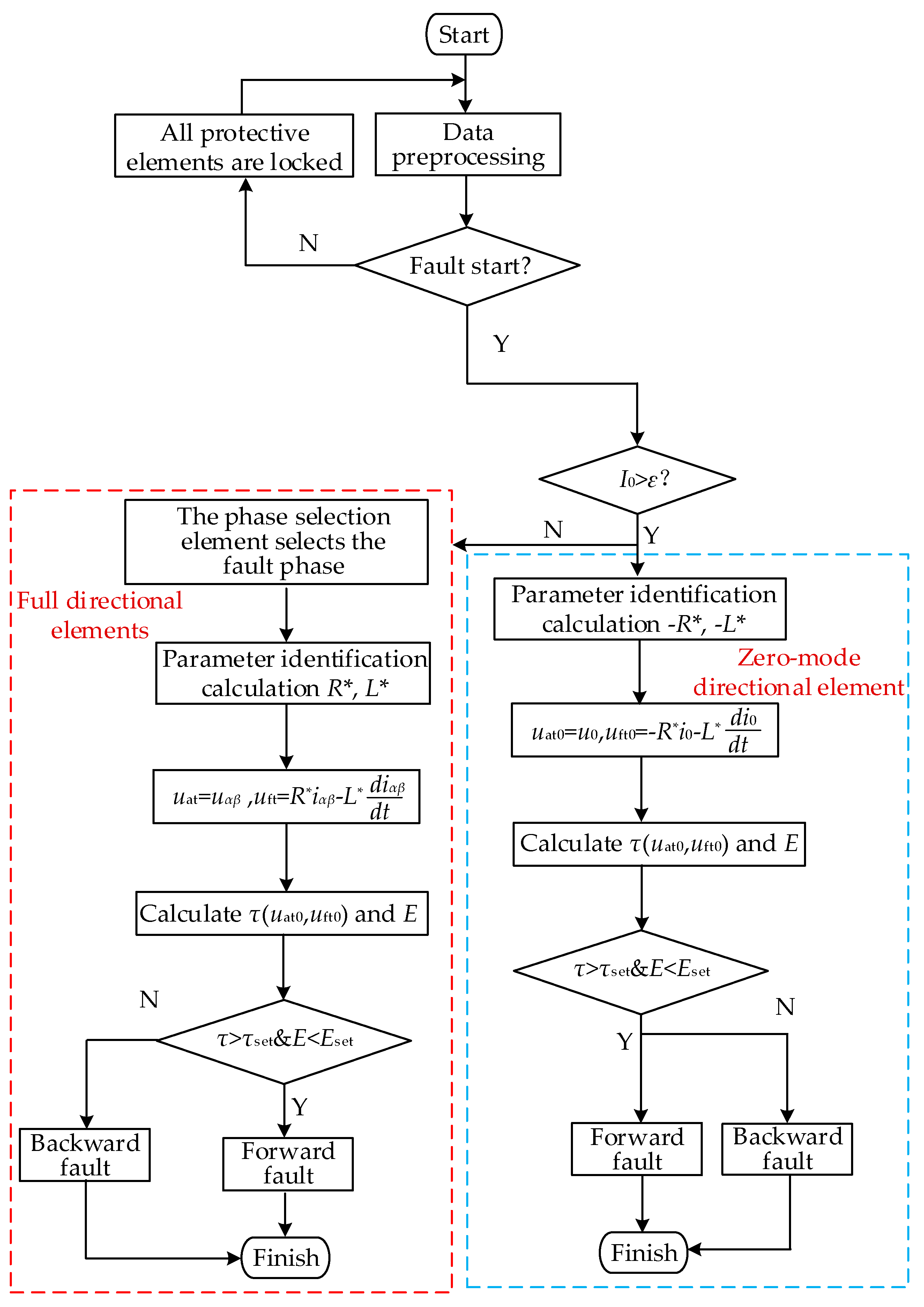
4.3. Protection Scheme

Building upon the established fault model and the comparative analysis between fitted and measured voltage characteristics, Figure 19 presents the proposed time-domain based fault direction identification methodology.

As shown in Figure 19, the direction component can be divided into the following steps:

(1)

The zero-mode current is calculated when a fault occurs on the outgoing line of a two-terminal weakly fed AC system. First of all, according to whether the fault instantaneous zero mode current meets the I₀ > ε criterion, determine whether it is a ground short circuit, and ε is the setting value; its value is very small and can be adjusted to ε_set = 0.1. If the conditions are met, the fault is a grounded short circuit. Otherwise, the fault is an ungrounded short circuit.

(2)

The fault phase is selected by the phase selector element and u and i are determined.

(3)

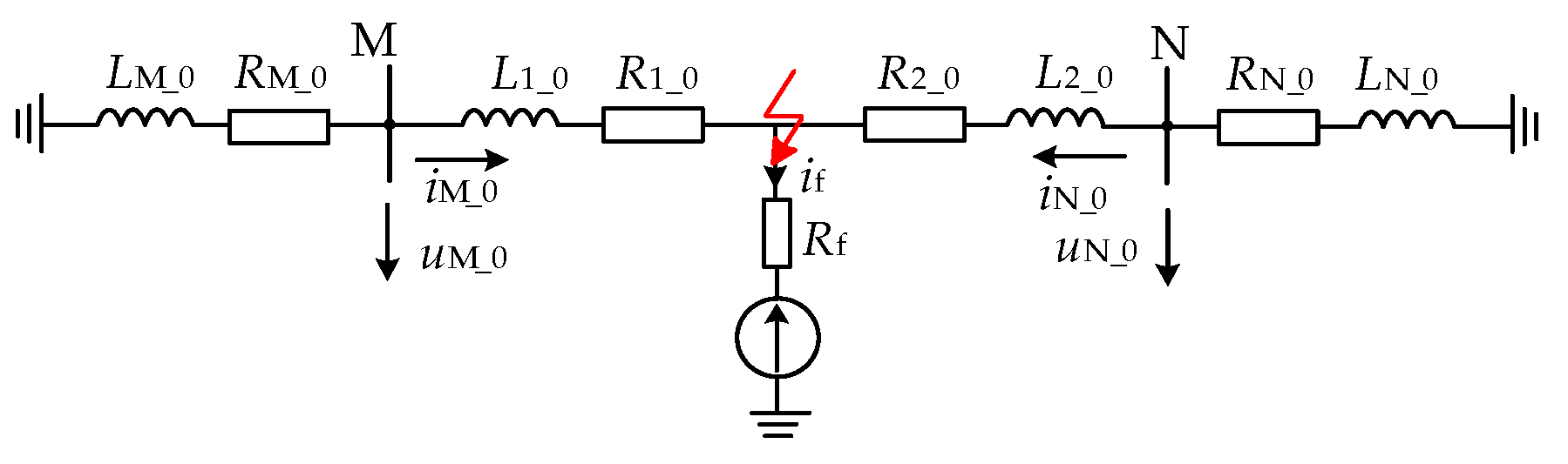
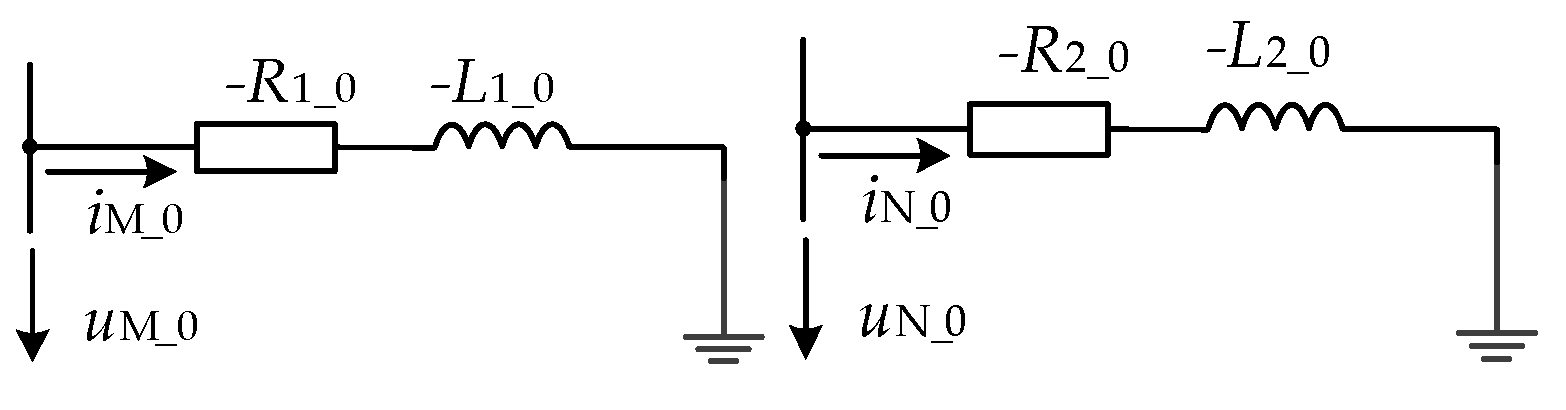
Assume that the fault occurs in the positive direction of the protection installation. Based on the parameter recognition algorithm, the equivalent resistance R* and equivalent inductance L* from the fault point to the protection installation point are calculated.

(4)

For ungrounded faults, the fault phase is used and the full direction criterion is used to judge the fault direction. For a ground fault, the zero-mode direction criterion is used to judge the direction of the fault.

(5)

For ungrounded faults, the correlation coefficient between the measured voltage and the forward fault fitting voltage is calculated, and the model error is calculated. For ground faults, the correlation coefficient between the zero-mode measured voltage and the zero analog combined voltage is calculated and the model error is calculated.

(6)

The relationship between the calculated Kendall coefficient τ and the average model error and the setting value is determined.

5. Simulation Verification

To validate the proposed protection scheme’s performance, a PSCAD/EMTDC simulation model was developed based on actual Chinese grid parameters, representing a PV plant with flexible direct grid integration (Figure 1). The model employs a 4 kHz sampling rate and features a 300 km 500 kV transmission line with the following per-unit parameters: positive-sequence (r₁ = 0.035 Ω/km, l₁ = 0.507 Ω/km) and zero-sequence (r₀ = 0.363 Ω/km, l₀ = 1.323 Ω/km) impedances.

5.1. Different Types of Fault Locations of Directional Element Action Performance Impacts

In order to verify the influences of different fault locations and fault types on directional components, different types of faults are set for f₁, f₃, and f₅ in the simulation model shown in Figure 1, and the discrimination results are shown in

Table 1. Directional component action performance for different fault types.

Fault Location	Fault Type	τM	$\widetilde{{\mathit{E}}_{\mathbf{M}}}$	Discriminant Result	τN	$\widetilde{{\mathit{E}}_{\mathbf{N}}}$	Discriminant Result
f1	AG	−0.9718	0.9999	B	0.9231	0.0422	F
	AB	−0.9872	0.9999	B	0.9590	0.0609	F
	ABG	−0.9923	0.9924	B	0.9974	0.0619	F
	ABCG	−0.9282	0.9999	B	0.9949	0.0664	F
f3	AG	0.9974	0.0702	F	0.9872	0.0554	F
	AB	0.9974	0.0151	F	0.9538	0.0338	F
	ABG	0.9923	0.0361	F	0.9949	0.0347	F
	ABCG	0.9359	0.0363	F	0.9974	0.0633	F
f5	AG	0.9538	0.0227	F	−0.9487	0.9804	B
	AB	0.9795	0.0214	F	−0.9897	0.9930	B
	ABG	0.9333	0.0498	F	−0.9974	0.9934	B
	ABCG	0.9997	0.0289	F	−0.9846	0.9999	B

. In the subsequent charts, “F” represents the faults in the forward direction and “B” represents the faults in the reverse direction.

Table 1 shows that the directional components in this chapter can operate reliably when different types of faults occur at different positions on the outgoing line of a two-terminal weakly fed AC system. The Kendall coefficient between the fitted voltage and the measured voltage is in accord with the model average error, and the proposed directional element can judge the direction reliably.

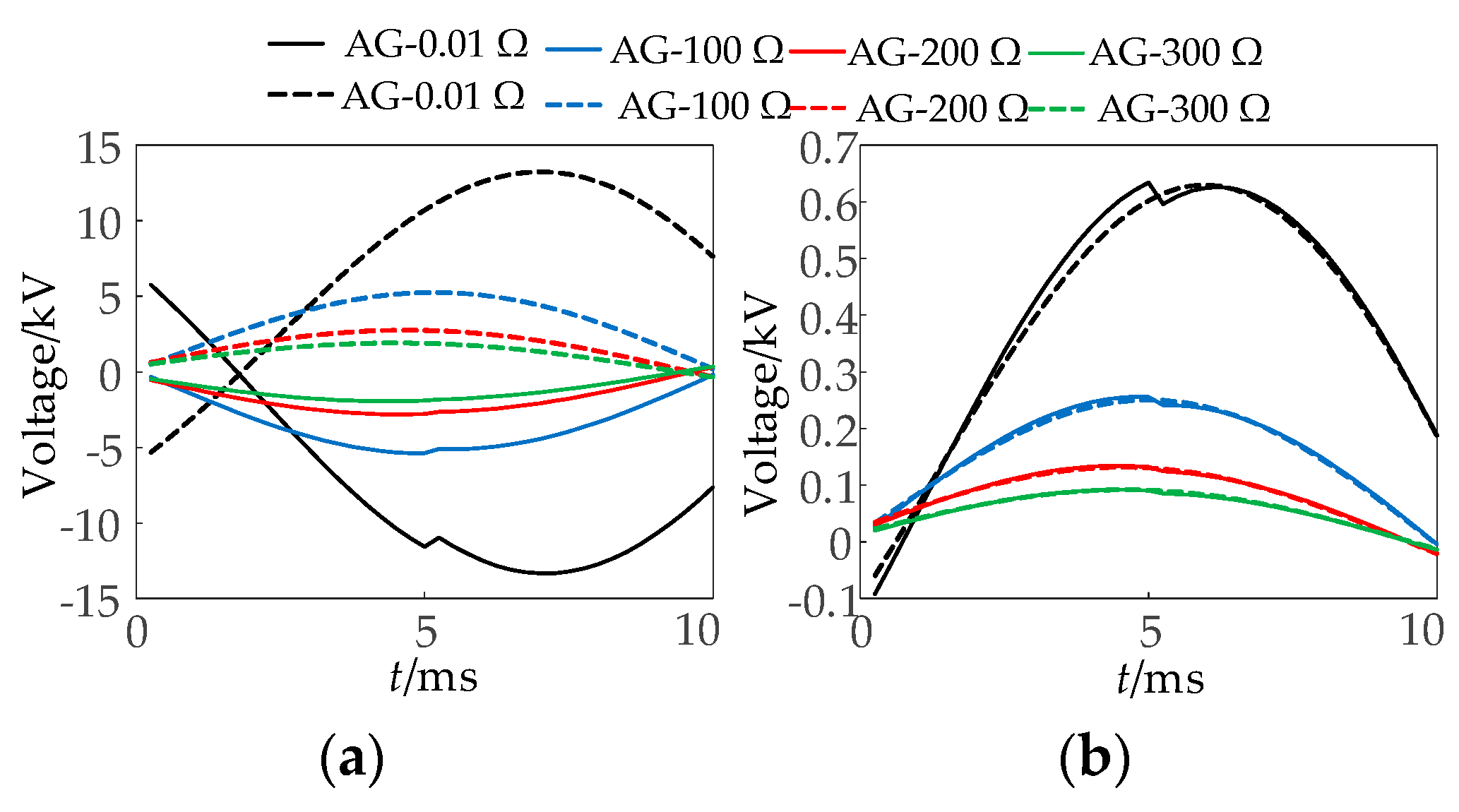
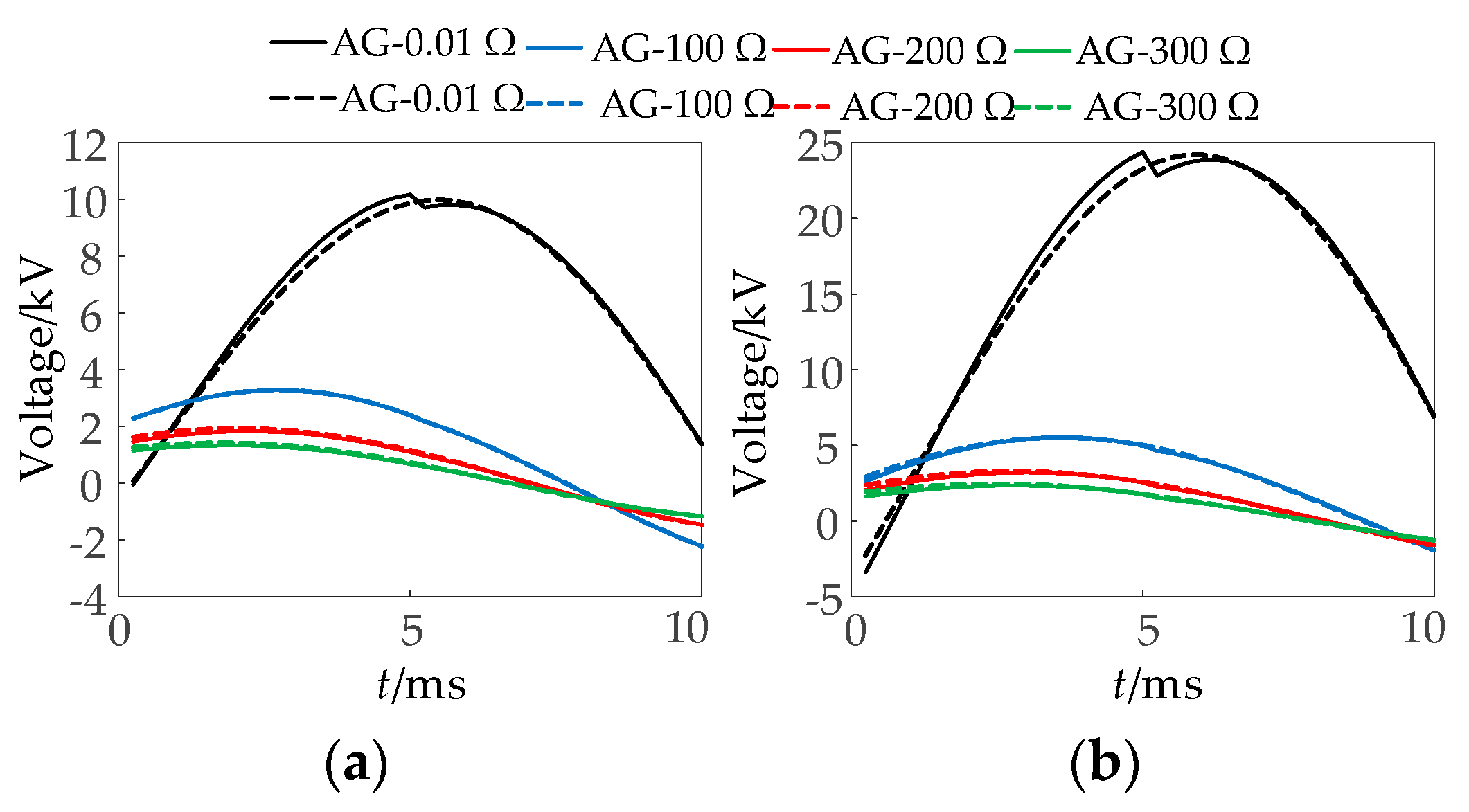
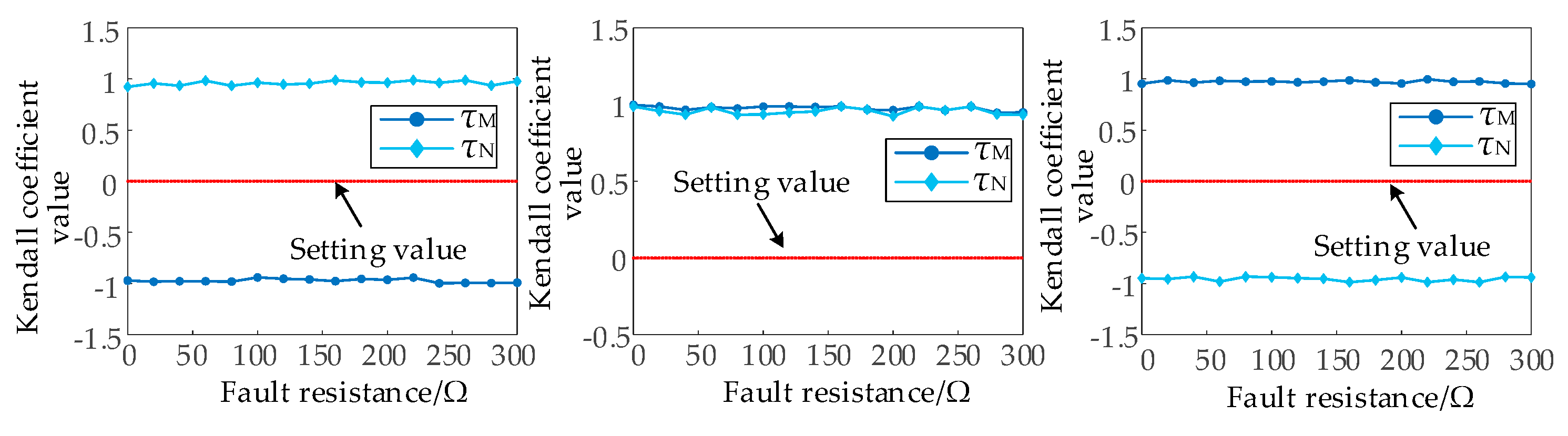
5.2. Different Transition Resistance Performances Influence the Motion of the Direction of Components

To evaluate transition resistance effects on directional protection, single-phase ground faults were simulated at points f₁, f₃, and f₅ (Figure 1) with resistances varying from 0.01 to 300 Ω. Figure 20, Figure 21 and Figure 22 compare the fitted (solid lines) versus measured (dashed lines) voltage relationships. Figure 23 presents the Kendall correlation coefficients, while

Table 2. Different transition resistances affect the action performance of the directional elements.

Fault Location	Transition Resistance	τM	$\widetilde{{\mathit{E}}_{\mathbf{M}}}$	Discriminant Result	τN	$\widetilde{{\mathit{E}}_{\mathbf{N}}}$	Discriminant Result
f1	0.01	−0.9718	0.9999	B	0.9231	0.0422	F
	100	−0.9410	0.9999	B	0.9641	0.0184	F
	200	−0.9641	0.9999	B	0.9641	0.0391	F
	300	−0.9923	0.9999	B	0.9769	0.0271	F
f3	0.01	0.9974	0.0702	F	0.9872	0.0554	F
	100	0.9462	0.0248	F	0.9359	0.0292	F
	200	0.9231	0.0454	F	0.9231	0.0455	F
	300	0.9487	0.0367	F	0.9333	0.0323	F
f5	0.01	0.9538	0.0227	F	−0.9487	0.9804	B
	100	0.9564	0.0174	F	−0.9385	0.9944	B
	200	0.9564	0.0164	F	−0.9410	0.9999	B
	300	0.9510	0.0163	F	−0.9410	0.9999	B

summarizes the fault direction identification outcomes.

As shown in Figure 20, Figure 21, Figure 22 and Figure 23 and Table 2, when the fault occurs at different fault locations and AG is short-circuited by the transition resistance, the Kendall coefficient value between the fitted voltage calculated by the integrated directional elements and the measured voltage is consistent with the model average error, and the proposed directional elements can reliably identify the direction. The directional elements presented in this paper can still operate reliably under a 300 Ω transition resistance.

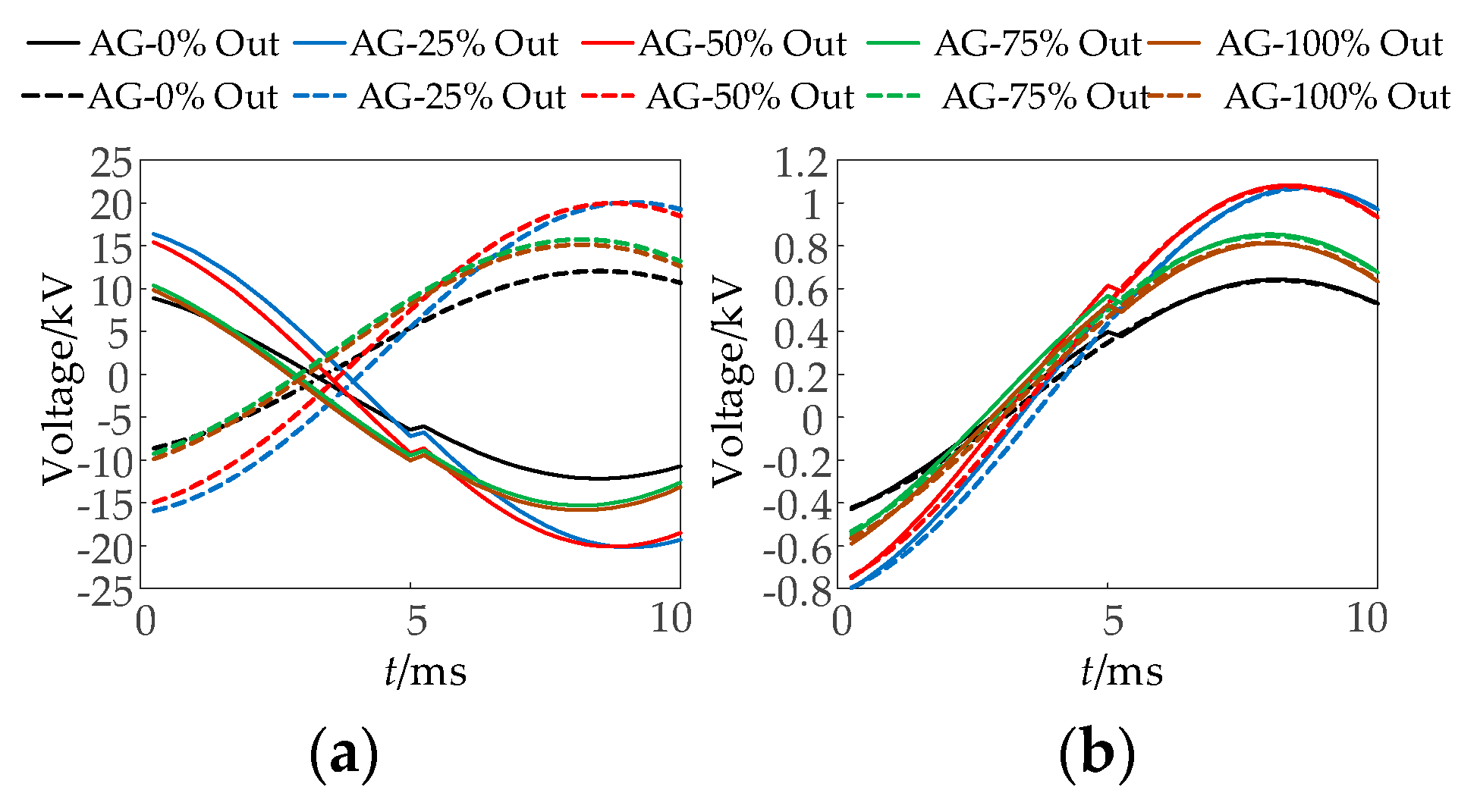
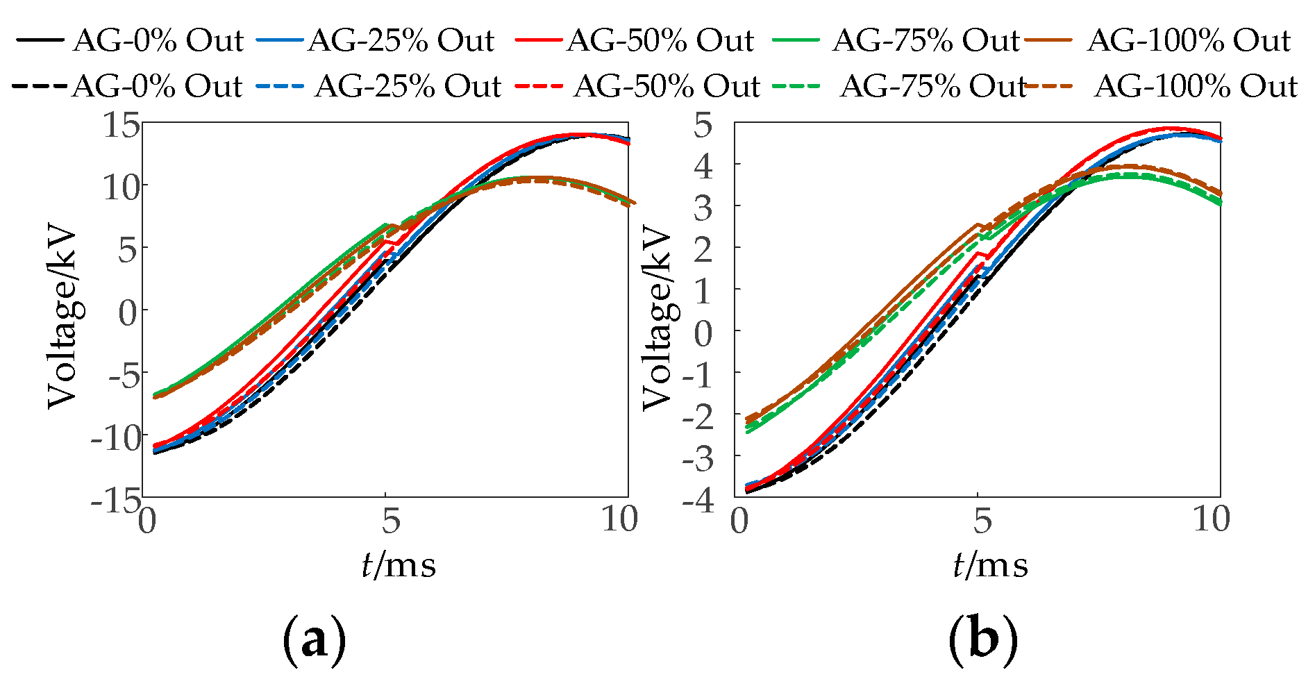
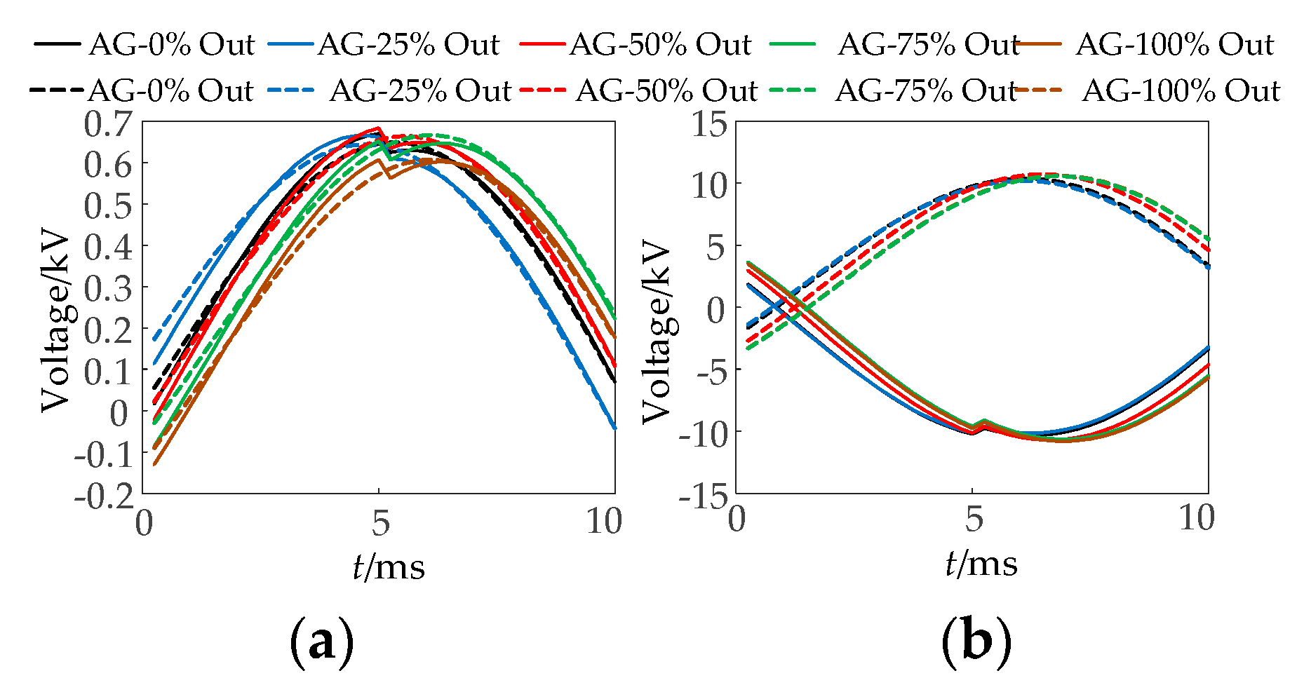
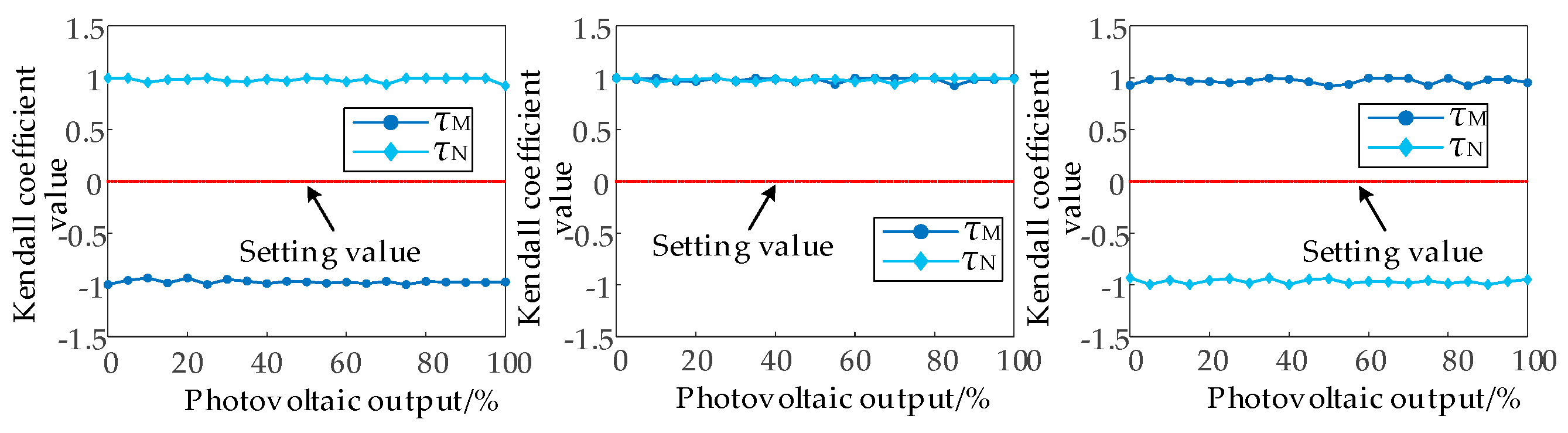
5.3. The Influence of Photovoltaic Output on the Directional Elements

This study evaluates photovoltaic generation impacts on directional protection by simulating ground faults at points f₁, f₃, and f₅ (Figure 1) under varying PV outputs (0–100% capacity), including zero-output nighttime conditions. Voltage measurement comparisons (fitted vs. actual values) are presented in Figure 24, Figure 25 and Figure 26, while Figure 27 displays the corresponding Kendall correlation coefficients.

Table 3. Different PV outputs influence the action performance of the directional elements.

Fault Location	Output	PM/nh	$\widetilde{{\mathit{E}}_{\mathbf{M}}}$	Discriminant Result	PN/nh	$\widetilde{{\mathit{E}}_{\mathbf{N}}}$	Discriminant Result
f1	0%	−0.9974	0.9884	B	0.9974	0.0350	F
	25%	−0.9970	0.9860	B	0.9974	0.0394	F
	50%	−0.9846	0.9912	B	0.9974	0.0311	F
	75%	−0.9974	0.9828	B	0.9974	0.0424	F
f3	0%	0.9974	0.0553	F	0.9974	0.0573	F
	25%	0.9974	0.0556	F	0.9974	0.0390	F
	50%	0.9951	0.0492	F	0.9872	0.0344	F
	75%	0.9978	0.0376	F	0.9974	0.0460	F
f5	0%	0.9282	0.0348	F	−0.9333	0.9999	B
	25%	0.9538	0.0327	F	−0.9410	0.9999	B
	50%	0.9205	0.0549	F	−0.9410	0.9999	B
	75%	0.9256	0.0652	F	−0.9590	0.9806	B

summarizes directional identification accuracy across five output levels (0%, 20%, 50%, 75%, and 100%).

As can be seen in Figure 24, Figure 25, Figure 26 and Figure 27 and Table 3, when the photovoltaic output is changed, the action performance of the directional components mentioned in this paper is not affected, and the fault direction can still be reliably identified. In actual life, the photovoltaic output will change with various factors. When the photovoltaic output is reduced, the directional element can still operate reliably.

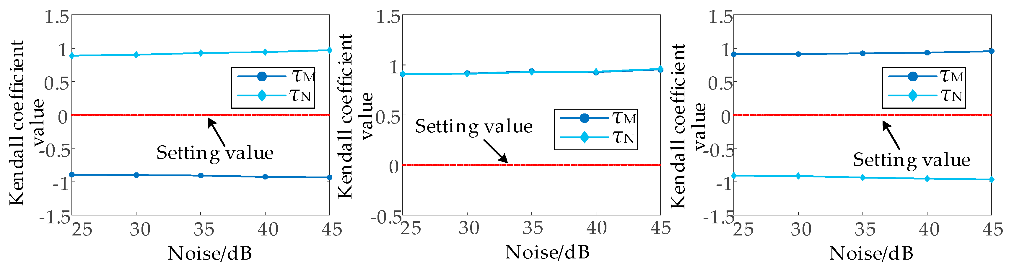
5.4. The Influence of Noise Interference on Directional Elements

This study investigates noise interference effects (25–45 dB range) on directional protection components through ground fault simulations at points f₁, f₃, and f₅ (Figure 1). Figure 28 presents the Kendall correlation coefficients quantifying the measurement consistency under noise conditions, while

Table 4. Different noise interference levels affect the action performance of the directional elements.

Fault Location	Noise	τM	$\widetilde{{\mathit{E}}_{\mathbf{M}}}$	Discriminant Result	τN	$\widetilde{{\mathit{E}}_{\mathbf{N}}}$	Discriminant Result
f1	25	−0.8952	0.9253	B	0.8874	0.0615	F
	35	−0.9075	0.9341	B	0.9288	0.0419	F
	45	−0.9360	0.9872	B	0.9692	0.0213	F
f3	25	0.9071	0.0446	F	0.9095	0.0413	F
	35	0.9386	0.0358	F	0.9296	0.0310	F
	45	0.9489	0.0262	F	0.9599	0.0211	F
f5	25	0.9093	0.0407	F	−0.9097	0.9698	B
	35	0.9237	0.0256	F	−0.9399	0.9754	B
	45	0.9553	0.0307	F	−0.9691	0.9885	B

details the directional discrimination accuracy at specific noise levels (25 dB, 35 dB, and 45 dB).

As shown in Figure 28 and Table 4, when white Gaussian noise with different SNRs is added to the discrete fitting voltage and measured voltage signals, the directional elements mentioned in this chapter can still correctly identify the fault direction. Considering the electromagnetic interference and other factors existing in the operating environment of the actual power line, the measured data show that the noise level of the line is generally not more than 25 dB. In this paper, the directional elements can still operate reliably under 25 dB of noise, which fully proves the reliability of the method.

5.5. The Influence of Control Strategies on Directional Elements

In order to verify the influence of different control strategies on the performance of directional components, different types of faults are set at the fault points of f₁, f₃, and f₅ in the simulation model in Figure 1, and the control strategies of PV inverters and MMC converters are changed. The judged results are shown in

Table 5. Operational characteristics of the directional protection elements under (1) negative-sequence current suppression at the PV terminal and (2) active power oscillation damping control at the MMC converter.

Fault Location	Fault Type	τM	$\widetilde{{\mathit{E}}_{\mathbf{M}}}$	Discriminant Result	τN	$\widetilde{{\mathit{E}}_{\mathbf{N}}}$	Discriminant Result
f1	AG	−0.9372	0.9651	B	0.9421	0.0422	F
	AB	−0.9152	0.9730	B	0.9765	0.0609	F
	ABG	−0.9823	0.9570	B	0.9873	0.0619	F
	ABCG	−0.9082	0.9834	B	0.9913	0.0664	F
f3	AG	0.9674	0.0257	F	0.9265	0.0554	F
	AB	0.9583	0.0348	F	0.9926	0.0338	F
	ABG	0.9765	0.0350	F	0.9987	0.0347	F
	ABCG	0.9219	0.0620	F	0.9564	0.0633	F
f5	AG	0.9682	0.0337	F	−0.9834	0.9504	B
	AB	0.9782	0.0254	F	−0.9109	0.9730	B
	ABG	0.9579	0.0438	F	−0.9043	0.99284	B
	ABCG	0.9999	0.0219	F	−0.9645	0.9999	B

,

Table 6. The behaviors of directional protection elements under dual control conditions: (1) negative-sequence current limitation in the PV system and (2) reactive power oscillation damping in the MMC converter.

Fault Location	Fault Type	τM	$\widetilde{{\mathit{E}}_{\mathbf{M}}}$	Discriminant Result	τN	$\widetilde{{\mathit{E}}_{\mathbf{N}}}$	Discriminant Result
f1	AG	−0.9108	0.9999	B	0.9240	0.0372	F
	AB	−0.9872	0.9999	B	0.9392	0.0489	F
	ABG	−0.9723	0.9924	B	0.9874	0.0549	F
	ABCG	−0.9182	0.9645	B	0.9518	0.0554	F
f3	AG	0.9670	0.0507	F	0.9272	0.0579	F
	AB	0.9526	0.0137	F	0.9649	0.0358	F
	ABG	0.9933	0.0471	F	0.9340	0.0374	F
	ABCG	0.9887	0.0283	F	0.9283	0.0620	F
f5	AG	0.9453	0.0227	F	−0.9487	0.9804	B
	AB	0.9325	0.0350	F	−0.9897	0.9930	B
	ABG	0.9632	0.0571	F	−0.9974	0.9934	B
	ABCG	0.9238	0.0352	F	−0.9846	0.9999	B

,

Table 7. The operational characteristics of directional protection elements are evaluated under (1) negative-sequence current limitation in the photovoltaic system and (2) reactive power oscillation damping in the modular multilevel converter.

Fault Location	Fault Type	τM	$\widetilde{{\mathit{E}}_{\mathbf{M}}}$	Discriminant Result	τN	$\widetilde{{\mathit{E}}_{\mathbf{N}}}$	Discriminant Result
f1	AG	−0.9618	0.9999	B	0.9520	0.0652	F
	AB	−0.9872	0.9872	B	0.9680	0.0327	F
	ABG	−0.9833	0.9340	B	0.9492	0.0619	F
	ABCG	−0.9745	0.9780	B	0.9983	0.0664	F
f3	AG	0.9572	0.0622	F	0.9752	0.0663	F
	AB	0.9860	0.0257	F	0.9838	0.0278	F
	ABG	0.9438	0.0387	F	0.9459	0.0317	F
	ABCG	0.9980	0.0452	F	0.9934	0.0729	F
f5	AG	0.9473	0.0195	F	−0.9583	0.9838	B
	AB	0.9385	0.0270	F	−0.9769	0.9728	B
	ABG	0.9952	0.0385	F	−0.9209	0.9928	B
	ABCG	0.9760	0.0270	F	−0.9871	0.9685	B

and

Table 8. Implementation of reactive power stabilization control in the photovoltaic system and negative-sequence current limitation strategy in the modular multilevel converter.

Fault Location	Fault Type	τM	$\widetilde{{\mathit{E}}_{\mathbf{M}}}$	Discriminant Result	τN	$\widetilde{{\mathit{E}}_{\mathbf{N}}}$	Discriminant Result
f1	AG	−0.9437	0.9720	B	0.9875	0.0422	F
	AB	−0.9713	0.9748	B	0.9735	0.0609	F
	ABG	−0.9782	0.9980	B	0.9482	0.0619	F
	ABCG	−0.9216	0.9999	B	0.9518	0.0664	F
f3	AG	0.9489	0.0512	F	0.9770	0.0482	F
	AB	0.9788	0.0270	F	0.9671	0.0348	F
	ABG	0.9405	0.0420	F	0.9878	0.0356	F
	ABCG	0.9950	0.0288	F	0.9920	0.0422	F
f5	AG	0.9386	0.0152	F	−0.9447	0.9784	B
	AB	0.9480	0.0078	F	−0.9259	0.9670	B
	ABG	0.9378	0.0362	F	−0.9416	0.9658	B
	ABCG	0.9536	0.0227	F	−0.9975	0.9999	B

.

It can be seen in Table 5, Table 6, Table 7 and Table 8 that upon the change in the control strategy of the photovoltaic inverter and MMC converter, the directional elements mentioned in this chapter can reliably identify the fault direction, which fully indicates that the method is not affected by the control strategy.

5.6. Comparison with Other Methods

The comparison of the operating performance of the directional elements mentioned in this chapter with the existing directional elements is shown in

Table 9. Method comparison.

Method	Whether It Is Affected by the Control Strategy	Withstands Transition Resistance	Tolerates Noise
[14]	Y	100 Ω	25 dB
[15]	Y	110 Ω	30 dB
[16]	Y	100 Ω	30 dB
[17]	Y	100 Ω	/
The method in this article	N	300 Ω	25 dB

.

6. Conclusions

In this paper, based on the research background of a two-terminal weakly fed AC system, directional elements for fault model differentiation discrimination in the time domain using the compound electrical volume are proposed.

(1)

The zero-mode voltage and current fault model under a ground fault and the full voltage and current fault model under non-ground fault are analyzed. The fitting voltage is constructed on the basis of the equivalent model, and the fault direction is determined by comparing the relationship between the fitting voltage and the measured voltage. The fitting voltage is the same as the measured voltage in the positive direction fault, and the fitting voltage is opposite to the measured voltage in the opposite direction fault.

(2)

The Kendall coefficient is introduced to calculate the correlation between the fitted voltage and the measured voltage, and the average model error is introduced to help judge the fault direction of the forward direction or the reverse direction. When a positive fault occurs, the Kendall coefficient between the fitted voltage and the measured voltage is close to one, and the average model error is close to zero. When the fault occurs in the opposite direction, the Kendall coefficient between the fitted voltage and the measured voltage is close to −1, and the average model error is close to 1.

(3)

The PSCAD/EMTDC model of a two-terminal weakly fed AC system was built to verify the performance of the proposed directional components for different fault types, fault locations, photovoltaic operating outputs, transition resistances, and control strategies. The results show that when the transition resistance is 300 Ω and the noise interference reaches 25 dB, the fault direction can still be correctly identified, which is suitable for a two-terminal weakly fed AC system.

References

1. Ding, M.; Wang, W.S.; Wang, X.L.; Song, Y.T.; Chen, D.Z.; Sun, M. A review on the effect of large-scale PV generation on power systems. Proc. CSEE 2014, 34, 1–14. [Google Scholar]
2. Zou, C.Y.; Wei, R.H.; Feng, J.J.; Zhou, Y.B. Development status and application prospect of VSC-HVDC. South. Power Syst. Technol. 2022, 16, 1–7. [Google Scholar]
3. Li, Y.; Luo, Y.; Xu, S.K.; Zhou, Y.B.; Yuan, Z.C. VSC-HVDC transmission technology: Application, advancement and expectation. South. Power Syst. Technol. 2015, 9, 7–13. [Google Scholar]
4. Feng, J.J.; Xin, Q.M.; Zhao, X.B.; Fu, C.; Yuan, Z.Y.; Huang, B.Y.; Zhou, Y.B.; Zhou, C.Y.; Hou, T. Integrated design scheme of VSC-HVDC system for large-scale renewable energy ultra-long-distance transmission. South. Power Syst. Technol. 2023, 18, 34–44. [Google Scholar]
5. Ji, X.T.; Liu, D.; Xiong, P.; Chen, Y.; Yang, L.; Wen, M.H. Survey of fault analysis and protection for power system with large scale power electronic equipments. Autom. Electr. Power Syst. 2024, 48, 140–149. [Google Scholar]
6. Yang, Q.F.; Liu, Y.Q.; Zhu, Y.M.; Chen, G.B. Improved Negative Sequence Directional Element for Transmission Line Connecting DFIG. Autom. Electr. Power Syst. 2019, 43, 118–126. [Google Scholar]
7. Niu, W.M.; Fan, Y.F.; Zhang, X.Y.; Ma, J. Novel parameter identification directional element based on impedance amplitude fluctuation difference. Power Syst. Prot. Control 2023, 51, 117–125. [Google Scholar]
8. He, J.H.; Wang, Y.R.; Li, M.; Du, X.T.; Yu, T.W. New Fault Direction Identification Based on Current Distortion Characteristics in High Proportion PV Distribution System. Power Syst. Technol. 2023, 47, 4856–4865. [Google Scholar]
9. Liu, W.; Lai, Q.H.; Liu, H.Y.; Zhang, Z.; Tan, Z.L. Novel method of fault direction identification for inverter-interfaced power supply access. Electr. Power Autom. Equip. 2020, 40, 205–212. [Google Scholar]
10. ALI, H.; REZA, I. A new directional element for microgrid protection. IEEE Trans. Smart Grid 2018, 9, 6862–6876. [Google Scholar]
11. Xu, G.J.; Liang, Y.Y.; Zha, W.T.; Huo, Y.T.; Qin, X.T.; Wang, C. Adaptability analysis of directional relay for transmission line out-sending from photovoltaic power plant. Power Syst. Technol. 2019, 43, 1632–1639. [Google Scholar]
12. Liang, Y.Y.; Lu, Z.J.; Li, W.L.; Huo, Y.T.; Xu, G.J.; Wang, C. Adaptability Analysis of Negative Sequence Directional Element and Cooperative Method With Control Strategy of MMC-HVDC. Power Syst. Technol. 2019, 43, 2998–3006. [Google Scholar]
13. Wu, L.P.; Wang, X.H.; Yan, D.; Ma, W.C.; Zhou, N.; Yu, H. Control Strategy for Fault Component Impedance Reconstruction of Flexible DC Converter Considering Relay Protection Requirement. Autom. Electr. Power Syst. 2023, 47, 110–119. [Google Scholar]
14. Tang, Y.; Shu, H.; Dai, Y.; Zhang, Y.; Han, Y. Pilot protection based on the quasi-directional element of LCL-tuned half-wavelength transmission line. Int. J. Electr. Power Energy Syst. 2023, 158, 109983. [Google Scholar] [CrossRef]
15. Xu, H.; Yin, C.; Dong, G.; Wang, S.; Xu, L.; Ouyang, F.; Zhu, W. Optimization of zero-sequence voltage compensation for zero-sequence directional elements. Electr. Power Syst. Res. 2021, 197, 107300. [Google Scholar] [CrossRef]
16. Chen, Y.; Wen, M.; Yin, X.; Cai, Y.; Zheng, J. Distance protection for transmission lines of DFIG-based wind power integration system. Int. J. Electr. Power Energy Syst. 2018, 100, 438–448. [Google Scholar] [CrossRef]
17. Ge, Y.Z. Principle and Technology of New Relay Protection and Fault Location; Xi’an Jiaotong University Press: Xi’an, China, 2007. [Google Scholar]
18. Wu, X.Q. Signal System and Signal Processing; Publishing House of Electronics Industry: Beijing, China, 1996. [Google Scholar]
19. Cong, W.; Zhang, H.; Kong, H.; Chen, M.; Wei, Z. Longitudinal Protection Method Based on Voltage Wave Comparison in AC/DC Hybrid System. IEEE Trans. Ind. Appl. 2022, 58, 1564–1572. [Google Scholar] [CrossRef]
20. Sadbhawna; Jakhetiya, V.; Chaudhary, S.; Subudhi, B.N.; Lin, W.; Guntuku, S.C. Perceptually Unimportant Information Reduction and Cosine Similarity-Based Quality Assessment of 3D-Synthesized Images. IEEE Trans. Image Process. 2022, 31, 2027–2039. [Google Scholar] [CrossRef] [PubMed]
Figure 1. Topology of large-scale renewable energy station through a flexible and straight grid connection system.
Electronics 14 02556 g001
Figure 2. Phase angle characteristics of equivalent positive-sequence impedance.
Electronics 14 02556 g002
Figure 3. Adaptability analysis of directional elements. (a) ZM1 and (b) ZM2.
Electronics 14 02556 g003
Figure 4. f3 ground fault zero-mode network model.
Electronics 14 02556 g004
Figure 5. f3 two-side zero-mode resistance inductance model under a ground fault.
Electronics 14 02556 g005
Figure 6. f5 ground fault zero-mode network model.
Electronics 14 02556 g006
Figure 7. f5 two-side zero-mode resistance inductance model under a ground fault.
Electronics 14 02556 g007
Figure 8. f1 ground fault zero-mode network model.
Electronics 14 02556 g008
Figure 9. f1 two-side zero-mode resistance inductance model under a ground fault.
Electronics 14 02556 g009
Figure 10. Ungrounded fault network model at f1.
Electronics 14 02556 g010
Figure 11. Ungrounded fault network model at f1.
Electronics 14 02556 g011
Figure 12. Ungrounded fault network model at f1.
Electronics 14 02556 g012
Figure 13. Ungrounded fault network model at f1.
Electronics 14 02556 g013
Figure 14. Ungrounded fault network model at f1.
Electronics 14 02556 g014
Figure 15. Ungrounded fault network model at f1.
Electronics 14 02556 g015
Figure 16. Ungrounded fault network model at f1.
Electronics 14 02556 g016
Figure 17. Ungrounded fault network model at f3.
Electronics 14 02556 g017
Figure 18. Ungrounded fault network model at f5.
Electronics 14 02556 g018
Figure 19. Directional element flow chart.
Electronics 14 02556 g019
Figure 20. Comparative waveforms of the fitted and measured voltages during Phase-A-to-ground faults at location f1 with varying transition resistances. (a) PV and (b) MMC.
Electronics 14 02556 g020
Figure 21. Comparative analysis of modeled versus actual voltage waveforms during Phase-A-to-ground faults at location f3 with varying transition resistances. (a) PV and (b) MMC.
Electronics 14 02556 g021
Figure 22. Comparative waveforms of the simulated and experimentally recorded voltages during a Phase-A-to-ground fault scenario at location f5, examining various transition resistance values. (a) PV and (b) MMC.
Electronics 14 02556 g022
Figure 23. The calculated values of τM and τN under the influence of transition resistance at different fault locations.
Electronics 14 02556 g023
Figure 24. The waveform diagram of the fitted voltage and measured voltage for different outputs of PV when an A phase ground fault occurs at f1. (a) PV and (b) MMC.
Electronics 14 02556 g024
Figure 25. The waveform diagram of the fitted voltage and measured voltage for different outputs of PV when an A phase ground fault occurs at f3. (a) PV and (b) MMC.
Electronics 14 02556 g025
Figure 26. The waveform diagram of the fitted voltage and measured voltage for different outputs of PV when an A phase ground fault occurs at f5. (a) PV and (b) MMC.
Electronics 14 02556 g026
Figure 27. Calculated values of τM and τN under the influence of the photovoltaic output at different fault locations.
Electronics 14 02556 g027
Figure 28. The calculated values of τM and τN under the influence of noise at different fault locations.
Electronics 14 02556 g028