Region Segmentation for Efficient Semiconductor Inspection: A Deep Learning Approach with Transformers and Atrous Convolution

Abstract

This paper explores the application of deep learning to automate the traditionally manual creation of inspection recipes for machine vision scenarios requiring complex region selection, such as those found in semiconductor manufacturing. Manually selecting and cropping functional regions in ultra-high-resolution images for analysis and inspection can take anywhere from tens of minutes to hours. To address this challenge, we propose a model whose encoder integrates atrous convolution into a transformer architecture for better feature extraction. This approach is designed to improve segmentation accuracy while maintaining efficiency in processing large-scale semiconductor images. By automating the selection and cropping process, the proposed method aims to streamline quality inspection workflows, reduce manual labor, and accelerate automated optical inspection. Experimental results demonstrate that the model achieves high segmentation performance, with segmentation accuracy reaching $98\%$ and a faster model inference, making it a practical and effective solution for enabling large-scale automation in semiconductor inspection. This research highlights the potential of deep learning-based methods to transform inspection processes, ensuring higher efficiency and product quality across semiconductor manufacturing industries.

1. Introduction

In industrial quality control, semantic segmentation plays a crucial role in automating processes, detecting anomalies, and ensuring product integrity. In semiconductor manufacturing, precise analysis of functional regions is essential for quality control, especially in complex components such as integrated circuits and Thin Film Transistor (TFT) backplanes. These regions must be carefully analyzed during the manufacturing process to ensure proper alignment and functionality. Currently, this process relies heavily on manual image selection and cropping, which is both time-consuming and labor-intensive. Creating a single Automated Optical Inspection (AOI) recipe can take several minutes to hours, significantly hampering manufacturing efficiency and scalability. This project aims to address these limitations by applying deep learning-based semantic segmentation to automate the selection and cropping of functional regions in semiconductor images, including TFT backplanes and other semiconductor components.

Deep learning models have proven effective in various sectors of the semiconductor industry, particularly in defect detection and quality control. For instance, ref. [1] employed deep convolutional neural networks (CNNs) to improve defect inspection in semiconductor wafer manufacturing. Similarly, prototype learning has been shown to efficiently handle defect segmentation in scenarios where background patterns vary [2]. These applications demonstrate the potential of deep learning to generalize well to unseen samples, providing more consistent and accurate results than traditional manual methods. Most of the existing literature on defect inspection in the semiconductor industry focuses on detecting small defects or performing image defect classification [3,4,5]. For instance, CNN-based methods have been successfully used for defect detection in printed circuit boards (PCBs) [6] and bubble segmentation in TR-PCBs (transmitter and receiver printed circuit boards) [7]. However, convolutional models, with their focus on local feature extraction, face limitations when applied to the segmentation of large-scale images typical of semiconductor applications. Our attempts to segment such high-resolution images using models like U-Net [8] and DeepLabV3+ [9] yielded unsatisfactory segmentation results as shown in Section 5. While these CNN-based methods have been valuable, they struggle with large-scale semantic segmentation tasks due to their limited receptive field and inability to model long-range dependencies. These shortcomings have motivated the exploration of transformer-based architectures, which use attention mechanisms to capture both local and global context more effectively.

Transformer-based models such as Vision Transformer (ViT) [10] and DETR [11] have since emerged as powerful alternatives in computer vision. By leveraging self-attention, they are better suited for tasks like image classification and object detection compared to convolution-based models [12,13]. Although ViT and DETR were initially applied to classification and detection, their strong performance demonstrated that transformers—originally developed for natural language processing—could also excel in vision tasks. This paved the way for their adoption in semantic segmentation, with SETR [14] being the first to use a pure transformer encoder, and TransUNet [15] introducing a hybrid architecture that combined transformers with convolutional decoders for medical image segmentation. These developments marked the beginning of the transformer era in segmentation, which has since become the dominant paradigm in the 2020s.

Building on this momentum, several advanced transformer-based segmentation models have been proposed. The Segment Anything Model (SAM) [16] introduces generalized zero-shot, interactive segmentation but lacks class-specific automation, making it less suitable for industrial AOI workflows. Swin-Unet [17], which integrates U-Net with a Swin Transformer [18] backbone, achieves excellent segmentation performance in medical images but suffers from slower inference due to its deep decoder. Other unified models, such as OneFormer [19] and Mask2Former [20], combine semantic, instance, and panoptic segmentation into a single architecture. While flexible, their complexity and computational demands make them impractical for high-throughput AOI systems that require only semantic segmentation.

Among existing models, SegFormer [21] offers an appealing balance between performance and efficiency. It uses a hierarchical transformer encoder with a lightweight decoder, enabling effective semantic segmentation with fewer parameters. When tested on our dataset, SegFormer outperformed CNN and other transformer models. However, SegFormer still has limitations. Its transformer layers are computationally demanding on high-resolution images, and it emphasizes global features at the expense of fine-grained local details—an important consideration in semiconductor inspection tasks that require precise boundary delineation.

To address these shortcomings, we propose a hybrid model that enhances SegFormer by integrating atrous convolutions into its encoder. This hybrid design leverages the global context modeling of transformers and the local feature extraction of convolutions, resulting in sharper segmentation masks and improved performance on fine structures. This modification not only enhances segmentation accuracy but also improves inference efficiency. Atrous convolutions are less computationally expensive than the transformer blocks they partially replace, reducing latency—an essential requirement for real-time industrial applications. Additionally, our method supports image downscaling during training and parallel processing of image patches, both of which contribute to substantial speed-ups during deployment. We also employ post-processing techniques to refine segmentation masks, extract contours, and identify points of interest (POIs), facilitating the automatic creation of AOI recipes. By automating the segmentation and cropping of functional regions in semiconductor images, our method drastically reduces manual effort and enhances throughput in high-volume manufacturing environments.

To the best of our knowledge, this work presents the first fully automated deep learning pipeline specifically designed for functional region segmentation in high-resolution semiconductor images, such as TFT backplanes. Unlike previous studies focused on defect classification or localized anomaly detection, our region segmentation approach enables a seamless integration into AOI automation, especially in cases where defects cannot be easily classified. The key contributions of this work are:

• A novel hybrid deep learning model whose encoder combines the hierarchical transformer of SegFormer with atrous convolutional networks. This design enhances local feature extraction while maintaining spatial resolution, resulting in sharper segmentation boundaries and improved overall segmentation accuracy for high-resolution semiconductor images.
• An optimized inference pipeline for large-scale, high-resolution images. The model supports flexible image downscaling—for example, from $2048\times 2048$ to $512\times 512$—during inference to accelerate processing while maintaining accuracy. It also uses patch-based batch inference, allowing multiple patches to be processed in parallel by leveraging available computational resources, significantly improving inference speed for large images.
• A post-processing algorithm that refines the segmentation masks to support AOI recipe creation. This algorithm removes false positives and false negatives from the masks and simplifies the extracted contours using polygonal approximation. This refinement enables the accurate extraction of regions of interest (ROIs) and points of interest (POIs), which are critical for downstream AOI tasks.

The remainder of this paper is structured as follows: Section 2 describes the AOI recipe creation process and explains how the segmentation model is integrated into the system. Section 3 presents the model architecture and the post-processing algorithms. Section 4 details the implementation on our dataset and the inference optimization strategies. Section 5 discusses the experimental results, and Section 6 concludes the paper.

2. AOI Recipe Creation

Automated Optical Inspection (AOI) recipes are predefined sets of inspection parameters or guidelines used in automated optical inspection systems to inspect and analyze manufactured components. AOI systems are commonly employed in high-precision industries, such as electronics, semiconductor manufacturing, and PCB (Printed Circuit Board) production, to ensure product quality and detect defects.

A critical component of the AOI recipe is the definition and selection of regions of interest (ROI). ROIs refer to specific areas of the component or image that the AOI system will focus on during inspection. These regions are selected to contain the most critical parts of the component, ensuring that the inspection effort is concentrated where defects are the most critical to the functions of the component or where issues are most likely to occur, while non-relevant areas are ignored. This process optimizes both the speed and accuracy of the inspection.

2.1. Current Manual ROI Selection Process

Currently, the process of selecting ROIs in the AOI recipe is performed manually, as illustrated in Figure 1. Operators use software tools to manually draw polygons around regions of interest, carefully outlining the functional areas that need to be inspected. While this method has been the standard for AOI recipe creation, it presents several challenges that hinder both the efficiency and scalability of the inspection process:

• Time-Consuming: Manually selecting regions for each inspection task can take anywhere from several minutes to hours, especially when dealing with high-resolution images of complex components. As the scale of production increases, the need to define a large number of regions and points manually becomes a significant bottleneck.
• Inaccuracy: High-precision tasks, such as inspecting semiconductor components or thin-film transistors (TFT), require an extremely accurate definition of regions. Even small deviations in the defined regions can lead to incomplete or incorrect inspections, potentially missing defects or causing false positives.
• Limited Scalability: As manufacturing processes scale up, the manual approach becomes increasingly unfeasible. Defining new regions and points for every new product or inspection scenario demands significant human intervention, which is not sustainable in high-volume production environments.

Figure 1. Manual selection and cropping of region of interest for AOI recipe creation.

Figure 1. Manual selection and cropping of region of interest for AOI recipe creation.

In addition to selecting regions of interest, points of interest (POIs) must also be manually defined in the AOI recipe. POIs are reference points that help the system determine the exact location of the inspection areas relative to other components in the image. These points are critical for ensuring alignment and correct positioning during the inspection process.

In the TFT Detection Recipe Editor (TFT-DRE) application, these POIs are manually placed by operators, as shown in Figure 2. Just like with ROI selection, manually defining POIs is also a time-consuming and error-prone task. Moreover, as the complexity of the component increases, such as with intricate semiconductor devices, the manual selection of these points becomes even more challenging and prone to inaccuracies.

2.2. Proposed Contribution of the Deep Learning Model

To overcome the inefficiencies and limitations of the current manual process, we propose integrating a deep learning-based segmentation model into the TFT-DRE application. The goal is to automate the definition of both ROIs and POIs, transforming the process from the one shown in Figure 3a to the streamlined version in Figure 3b. This integration offers several key improvements:

• Automated ROI Selection: The deep learning model will be trained to automatically identify and segment relevant regions of interest in high-resolution images. Instead of relying on operators to manually outline functional regions, the model will analyze the images and generate accurate segmentations of areas that require inspection, eliminating the need for manual polygon creation.
• Enhanced Accuracy and Consistency: The deep learning model can offer higher precision in defining regions and points, ensuring consistent and reliable inspections. Unlike manual methods, which are prone to human error, the model can analyze complex patterns and relationships within the image with greater accuracy, leading to more precise defect detection and fewer false positives or missed defects.
• Scalability and Flexibility: Once trained, the model can be easily applied to a wide range of components and inspection scenarios. This will allow for rapid deployment of AOI recipes for different products without requiring the manual definition of new ROIs and POIs each time. The model can also be adapted to new inspection tasks as needed, making it a versatile tool for high-volume manufacturing environments.
• Speed and Efficiency: By automating the regions and points selection process, the model will significantly speed up the creation of AOI recipes. This will result in faster setup times and reduced downtime, allowing for more efficient inspection workflows and quicker adaptation to new production requirements.
• Continuous Improvement and Adaptation: As the model is exposed to more data over time, it can be retrained and fine-tuned to handle new components resulting from different manufacturing variations or imaging conditions. This makes the system adaptable and capable of improving as new inspection challenges arise.

Figure 3. Flowchart of the selection of ROIs and POIs in AOI system (manual vs. automatic processes). (a) Manual selection of ROIs and POIs. (b) Automatic selection of ROIs and POIs using a segmentation model.

Figure 3. Flowchart of the selection of ROIs and POIs in AOI system (manual vs. automatic processes). (a) Manual selection of ROIs and POIs. (b) Automatic selection of ROIs and POIs using a segmentation model.

3. Methodology

Our approach to effective application of deep learning to the creation of AOI recipes involves five key steps: preparing the training data, defining the model architecture, training the model on the dataset, testing the model on unseen images, and post-processing the segmentation masks to extract the contours of the ROIs and the coordinates of the POIs. For the segmentation, we propose a deep learning-based segmentation model that combines transformers and atrous convolution with a Multi-Layer Perceptron (MLP) decoder. This architecture is designed to effectively segment the ROIs, and the POIs are subsequently determined based on the segmented ROIs, which are crucial in the AOI recipe creation process. In this section, we define the model’s architecture and describe the post-processing techniques used to extract the ROIs and POIs. The steps related to preparing the data, training the model, and testing the model on unseen images will be covered in the Implementation (Section 4).

3.1. Segmentation Model

3.1.1. Encoder Design

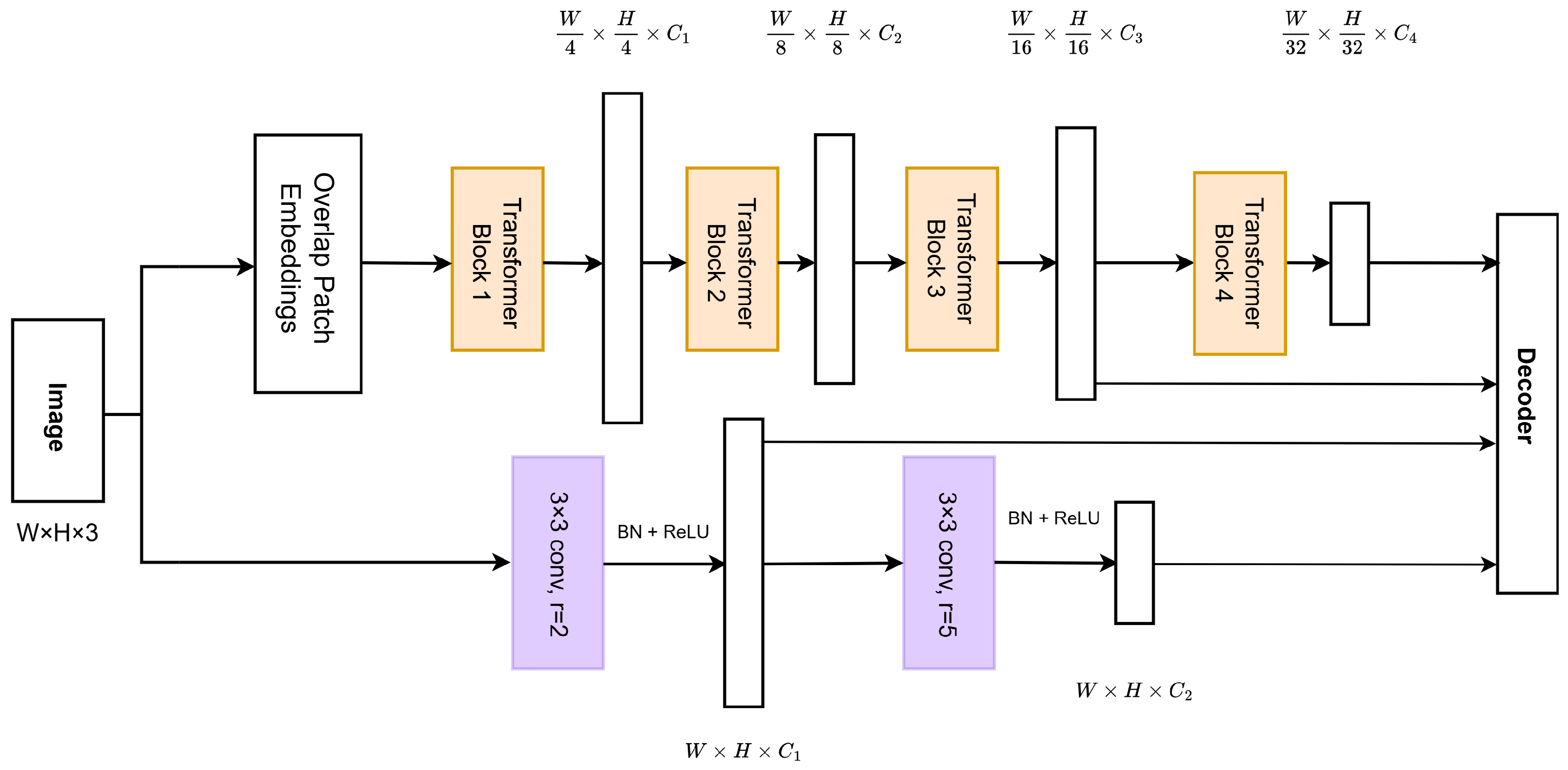
The encoder, as shown in Figure 4, features a hybrid design with two parallel paths: a transformer path similar to SegFormer’s encoder and a convolutional network path utilizing dilated convolutions. This hybrid architecture is designed to combine the strengths of both transformers and convolutions to improve both local and global feature extraction capabilities.

This approach was considered after observing that, when training both DeepLabV3+ and SegFormer-B0 on our dataset, the models performed differently across classes and had varying effects on the edges of the predicted segmentation maps. The goal was to maintain the high overall segmentation accuracy that SegFormer provided, while improving the accuracy of specific classes, particularly, the definition of the edges of the under-represented classes that SegFormer struggled with. Additionally, we aimed to enhance the definition of the edges in the segmentation maps, which were better defined by DeepLabV3+ compared to SegFormer.

The transformer block used here is the efficient self-attention block [21]. It reduces the computational requirement of transformers and aligns with our aim to develop a model for fast inference. The efficient self-attention block is a computationally optimized version of the original scaled dot product attention from [22] estimated as:

$$\mathrm{Attention}(Q,K,V)=\mathrm{Softmax}\left({\displaystyle \frac{Q{K}^T}{\sqrt{d_k}}}\right)V$$

(1)

where Q is the query matrix, K the key matrix, V the value matrix, and ${\displaystyle \frac{1}{\sqrt{d_k}}}$ is a scaling factor, $Softmax\left(z_i\right)={\displaystyle \frac{e^{z_i}}{{\sum }_j{e}^{z_j}}}$. In the original transformer paper [22], for heads of dimension $N\times C$ where $N=H\times W$, the computational complexity is $O\left(N^2\right)$. The efficient self-attention from [23] reduces the complexity to $O\left({\displaystyle \frac{N^2}{R}}\right)$ by decreasing the spatial dimensions of the input sequence. Specifically, it performs the following transformation:

$$K=\mathrm{Linear}(C·R,C)\left(\mathrm{Reshape}\left({\displaystyle \frac{N}{R}},C·R\right)\left(K\right)\right)$$

(2)

which reduces the dimension of K to ${\displaystyle \frac{N}{R}}\times C$.

• where: R is a reduction ratio. $Reshape(X,Y)\left(K\right)$ means reshaping K to have the shape $X\times Y$, $Linear\left(C_{in},C_{out}\right)(·)$ refers to a linear layer taking a $C_{in}$-dimensional tensor as input and generating a $C_{out}$-dimensional tensor as output, $N\times C$ are the dimensions of each of the heads $Q,K,V$.
• $N=H\times W$ is the length of the sequence, height and width of the image or patch and C is the channel dimension.

The transformer path in the proposed model closely follows the structure of SegFormer’s encoder, which processes the input image through four stages. Each stage progressively reduces the spatial resolution while increasing the semantic richness of the feature maps. However, in our design, only the outputs of the last two stages (with channels $C_3$ and $C_4$) are passed to the decoder. The first stages are replaced by convolution blocks that are more efficient at extracting local features compared to the transformer blocks.

The convolution blocks used here are dilated convolution. The choice of the dilated convolution blocks was inspired by their use in DeepLabV3+, and the general ability of convolutional networks to better extract local features. We opted for atrous convolution instead of standard convolution to slightly expand the receptive field, facilitating a smooth transition from convolution to transformer layers, without increasing the kernel size, which would add more parameters to the model.

The output $y\left[i\right]$ of a dilated convolution for a one dimensional input $x\left[i\right]$ with a filter $w\left[k\right]$ of length K is defined as:

$$y\left[i\right]=\sum _{k=1}^{K}x[i+r·k]w\left[k\right]$$

(3)

where r is the dilation rate.

In this context, $x\left[i\right]$ represents a data point in the input sequence x, with i being the index of each element of x. w is the convolution kernel (or filter) of length K, and it contains the weights applied to the input sequence x to compute the output $y\left[i\right]$ The dilation rate r determines the spacing between the elements of the filter as it convolves over the input sequence. When $r=1$, the operation reduces to a standard convolution, where each filter element interacts with consecutive input element. For higher values of r, the filter elements are spaced apart by r positions in the input sequence, effectively enlarging the receptive field without increasing the kernel size. To compute the output $y\left[i\right]$, the weighted sum of the input values $x[i+r·k]$ is calculated, with the indices determined by the dilation rate. For example, consider a sequence $x=[x_1,x_2,x_3,x_4,x_5]$, a kernel $w=[w_{1,}{w}_2,w_3]$, and a dilation rate $r=2$. The output is given by: $y\left[i\right]=x[i+2·1]w\left[1\right]+x[i+2·2]w\left[2\right]+x[i+2·3]w\left[3\right]$. In this case, the kernel elements are spaced by 2 positions, meaning the corresponding input elements are selected with gaps in between. When the indices $i+r·k$ exceed the range of the input sequence, or when early input elements are not involved in the computation, the input sequence is zero-padded at the boundaries to handle these cases.

The convolution path consists of two dilated convolution blocks, designed to produce feature maps with channel dimensions matching those of the first two transformer stages ($C_1$ and $C_2$, respectively). The dilated convolution blocks preserve spatial resolution while expanding the receptive field, allowing them to extract features across multiple scales without losing geometric integrity. The outputs of the convolutional path are used to replace the outputs of the first two transformer stages in the encoder’s final output.

The outputs of the convolutional path (representing the first two stages) are concatenated with the outputs of the last two transformer stages. This combined output, with shape $H\times W\times 4C$ (where $4C$ is the total channel dimension from all four stages), is passed to the decoder for feature upsampling and segmentation mask prediction.

To summarize, the hybrid encoder design addresses specific challenges observed with existing models, when applied to our dataset:

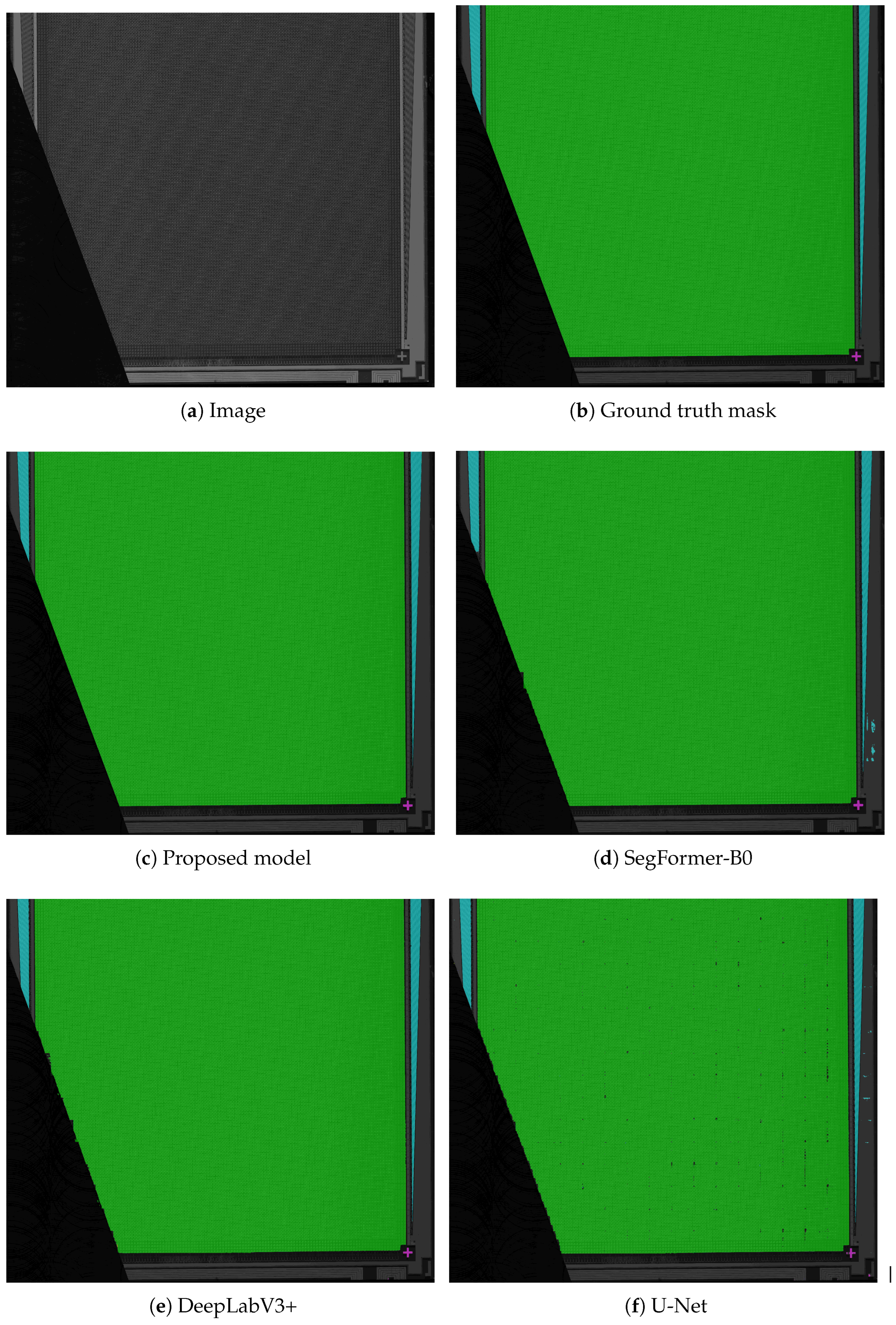
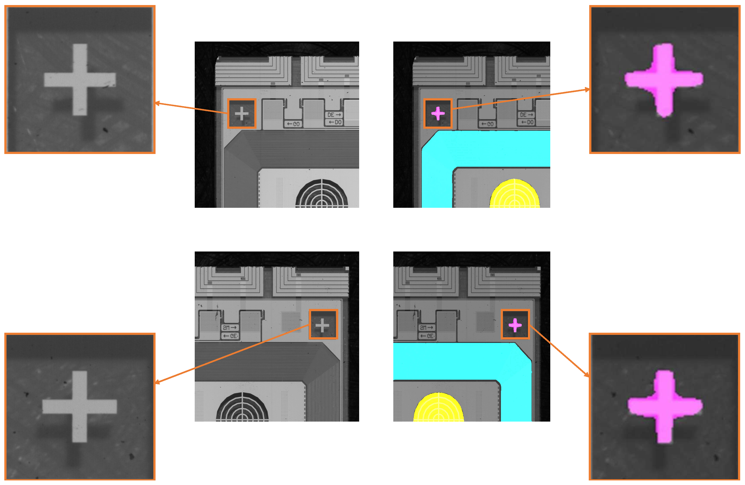
• Boundary irregularities in segmentation maps: While SegFormer achieves high segmentation accuracy, its segmentation maps suffer from boundary irregularities. In particular, edges that should be sharp and straight, such as those in the alignment crosses in Figure 5, instead exhibit watershed-like effects where edges deviate from expected straight-line structures. As shown in the figure, the lack of sharpness in the segmentation map makes the output unsuitable for practical applications. Even post-processing techniques fail to correct these irregularities, further limiting the usefulness of the model for automated region selection. This problem is not limited to alignment references only, but is also observed across other segmentation classes.
• Transformers’ Weakness in Fine-Grained Details: Although the hierarchical transformer encoder excels at extracting local and global features, the self-attention mechanism in its early stages tends to emphasize global relationships across the feature map. This can blur small, precise structures, such as sharp edges, as seen in the segmentation maps in Figure 5.
• Convolutions for Spatial Preservation: Convolutions, by contrast, inherently encode spatial locality, making them better at detecting and preserving fine-grained structures such as edges. The dilated convolutions used in our convolution path further enhance the ability to capture multi-scale features without losing geometric integrity by assigning different dilation rates to the two convolution blocks. To ensure that the spatial dimensions remain constant throughout the convolutional path, we carefully adjust the dilation rates and padding values in each dilated convolution block. This design allows the convolution path to extract features across scales while preserving the original spatial resolution, ensuring that no information is lost at the edges or in smaller regions. By maintaining constant spatial dimensions, the convolutional path eliminates the need for upsampling operations, which are required in the transformer path to restore reduced spatial dimensions. This not only simplifies the decoder design but also reduces computational overhead during inference.
• Efficiency: The convolution blocks are computationally lighter than the transformer blocks they replace, simplifying the model for faster inference. Their ability to retain spatial resolution without requiring additional upsampling further contributes to the model’s efficiency.

3.1.2. Decoder Design

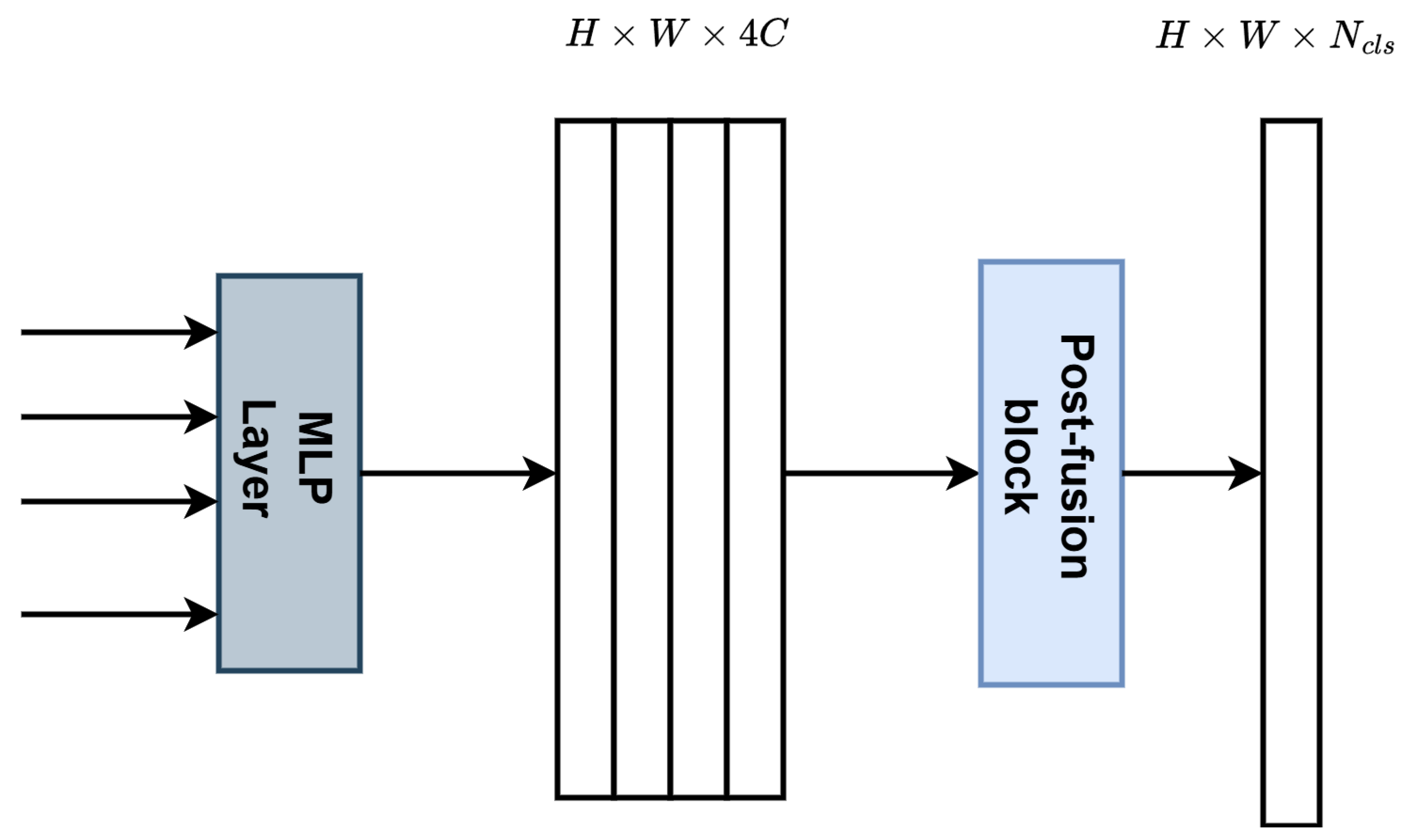
The decoder, as shown in Figure 6, consists of two main components: the MLP Layer and the Post-fusion Block.

The MLP Layer processes the feature outputs from the four encoder stages. In this layer, each feature map is first passed through a convolutional projection to unify the channel dimensions to a consistent size (C). The projected feature maps are then upsampled to match the spatial resolution of $H\times W$. Once aligned and upsampled, the feature maps are concatenated along the channel dimension to form a single tensor with the shape $H\times W\times 4C$. This concatenation allows the decoder to effectively combine multi-scale information from the different encoder stages.

In the post-fusion block, the concatenated features undergo a series of operations to refine them. First, the features are passed through batch normalization, which normalizes the activations across the batch. Then, a ReLU activation function introduces non-linearity to the model, followed by dropout to prevent overfitting. After these operations, the number of channels is reduced from $4C$ to $N_{cls}$, where $N_{cls}$ is the number of segmentation classes, using a $1\times 1$ convolution. This final convolution generates the pixel-level classification map (logits) with the shape $H\times W\times N_{cls}$, which corresponds to the predicted segmentation mask.

3.2. Post-Processing of Segmentation Masks

After obtaining the results of the segmentation process, the segmentation masks are analyzed using computer vision and digital image processing techniques to extract the ROIs and POIs necessary for the AOI recipe creation. The focus of these techniques is on detecting the contours of each class in the segmentation mask and approximating them with polygons, which simplifies the extraction of ROIs and POIs.

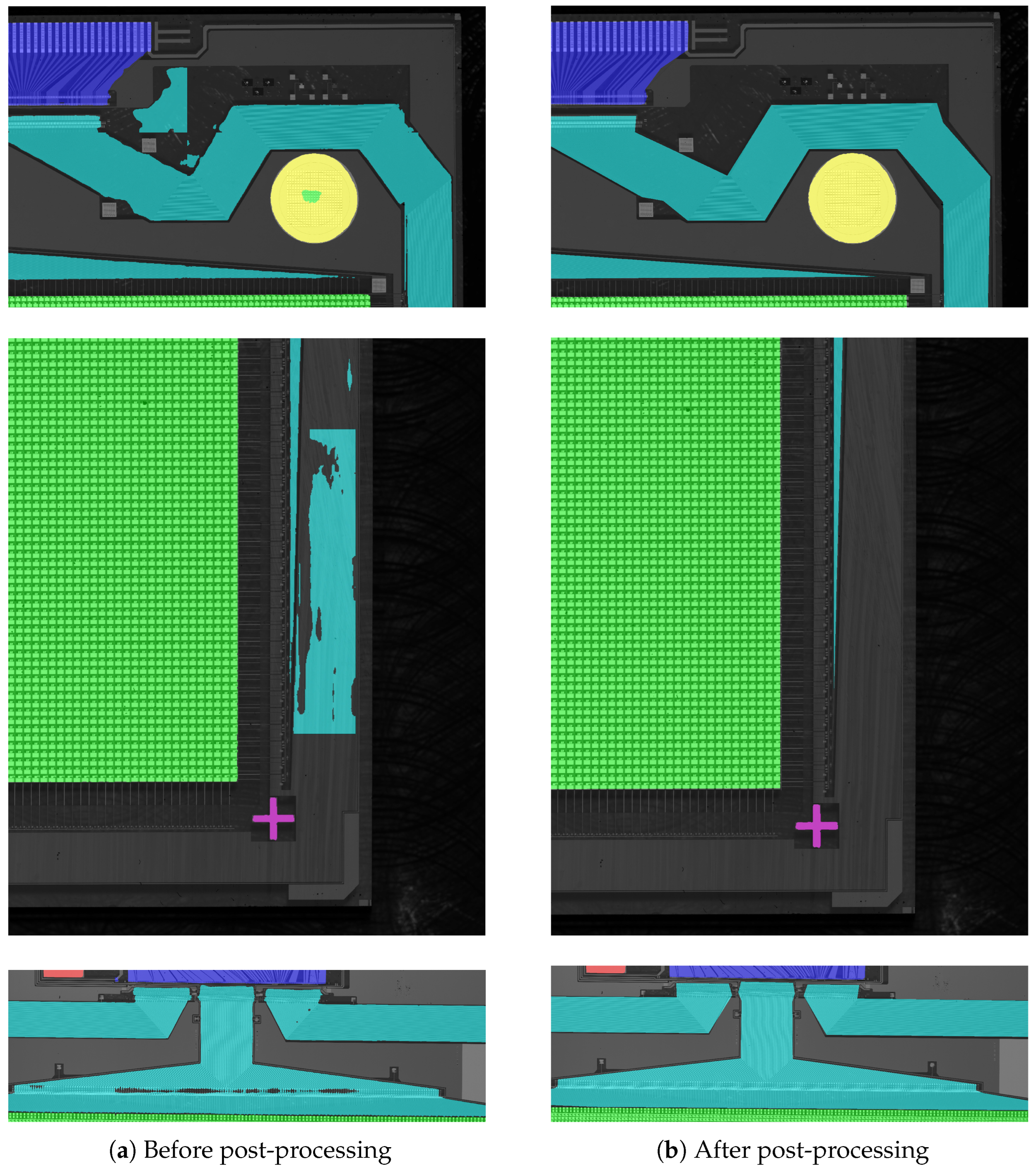
The steps involved in contour simplification and POI extraction are outlined in Algorithm 1. In step 1, the conversion of the segmentation masks from RGB to HSV (Hue, Saturation, Value) color space allows for better separation of the regions based on color. By separating color (Hue) from brightness (Value), this improves the algorithm’s ability to identify distinct classes more effectively. From steps 2 to 4, each segmentation class is classified based on its unique HSV values, and individual class contours are identified. The number of contours for each class is calculated and false positives—regions incorrectly assigned to a class—are eliminated. A false positive occurs when a region is mistakenly classified as part of one class, but it does not belong there, such as in the case where the AA or background class is incorrectly identified as part of the IC class.

In step 5, false negatives are addressed using contour hierarchy to detect nested contours. False negatives occur when regions that should belong to a class are missed, often due to them being incorrectly labeled or not detected at all. Using contour hierarchy, child contours fully enclosed by parent contours are discarded, ensuring only valid, larger contours are retained.

To prevent contours from different classes merging, the algorithm processes each class individually, repeating Steps 3 to 5 for each class. This guarantees that contours are correctly associated with the appropriate class, avoiding merging across classes.

After eliminating false positives and false negatives, the contours are simplified in step 7 using the Ramer–Douglas–Peucker (RDP) algorithm which reduces the number of vertices while preserving the overall shape of the contours, making them easier to edit when misalignment occurs between the polygon and the area of interest. The POIs are detected and stored along with the vertices of the polygons.

Algorithm 1 Pseudocode of post-processing of segmentation maps to extract ROIs and POIs

1: Step 1: Convert the segmentation map from RGB to HSV color space   2: Use OpenCV to convert the image from RGB to HSV   3: Step 2: Identify classes and their assigned HSV colors in the segmentation map   4: Extract unique HSV color values   5: Assign each color to a corresponding class   6: Step 3: For each class in the segmentation map:   7:    Isolate segments of the class using its HSV color   8:    Find contours of the class instances   9:    Count the number of contours as the number of predicted instances 10: Step 4: Eliminate false positives: 11:    For each contour, calculate the enclosed area $A_{contour}$ 12:    Calculate the threshold area $A_t$ using: $$A_t=\lambda \times A_{\max }$$ 13: where $\lambda$ is the minimum area ratio, $A_{max}$ is the largest area among the contours. 14:    If $A_{contour}$<$A_t$, discard the contour 15: Step 5: Eliminate false negatives: 16:    Use contour hierarchy to detect nested contours 17:    Discard child contours that are fully enclosed by parent contours 18:    Retain only parent contours for valid instances 19:    Also discard false positives from other classes if not removed in Step 4 20: Step 6: To prevent contour merging of different classes: 21:    For each class, repeat Steps 3–5, analyzing one class at a time 22: Step 7: Simplify the contours 23: Use Ramer–Douglas–Peucker algorithm to approximate the contours with polygons have less vertices 24: Detect the POIs and save them along with the coordinates of the vertices 25: Step 8: Draw the polygons on the original image 26: Fill the polygons using alpha blending for transparency such that the structures of the image can be seen through the mask 27: The blended image is computed using the formula: $$imag{e}_{blended}=\alpha \times mask+(1-\alpha )\times image$$ 28: where $\alpha \in (0,1)$ controls the transparency level of the blended image 29: Step 9: Display the blended image for user editing when needed 30: Make the vertices of the polygons more pronounced, the enlarged vertices are easy to be spotted and edited if needed. 31: Step 10: Send the vertices and POIs to inspection stage

The RDP algorithm simplifies polygons by reducing the number of vertices while retaining the overall shape. This method is particularly useful in contour simplification for segmentation masks. The algorithm works by recursively eliminating points that lie within a defined tolerance $ϵ$ from the line segment joining adjacent points.

To improve the quality of the contours for user editing, the tolerance value, $ϵ$, is dynamically adjusted based on the polygon’s area. Smaller areas are simplified with a higher $ϵ$ while larger areas are simplified with a lower $ϵ$, preserving more of the original shape. This approach is governed by the equation:

$$ϵ={ϵ}_{min}+({ϵ}_{max}-{ϵ}_{min})\times e^{-kA}$$

(4)

where ${ϵ}_{\max }$ and ${ϵ}_{\min }$ are experimentally determined, and A is the polygon’s area. In our implementation, ${ϵ}_{\max }=2\times {10}^{-2}$, ${ϵ}_{\min }={10}^{-3}$, and $k={10}^{-5}$.

The values of ${ϵ}_{\max }$, ${ϵ}_{\min }$, and k were determined empirically, taking into account the surface areas of the various ROIs in the dataset, as well as the approximate number of vertices needed to accurately represent the contours of each ROI. These estimates were based on observations made during both the image annotation phase and model testing. Since most ROIs exhibit relatively well-defined geometric shapes, we were able to approximate the number of vertices required to describe their contours using a few representative examples.

Once simplified, the contours are drawn on the original image in step 8, with the polygons filled using alpha blending for transparency. This allows the underlying structures of the image to remain visible through the mask, providing a clear view of the segmentation result. The blended image is then displayed in step 9 for user editing. The vertices of the polygons are highlighted to make them easier to spot and adjust if necessary. Finally, in step 10, the vertices and POIs are sent to the inspection stage, where they are used to guide the inspection process and identify defects in the corresponding ROIs.

4. Implementation

We implemented the proposed model by training it on a custom dataset created with TFT backplane images. We then further implemented techniques to expedite the inference time and compared our segmentation results to other models such as U-Net, DeepLabV3+, and SegFormer-B0.

4.1. Image Acquisition System

The images used for training and evaluation were acquired using a commercial Automated Optical Inspection (AOI) system, model HIO-FPD-A1, developed by HIO Technology (Huzhou) Ltd. (Huzhou, China) This system is purpose-built for high-resolution imaging of TFT backplanes in display screens. It supports a magnification range of $1.2\times$ to $1.7\times$ and employs line-scan imaging to generate ultra-high-resolution images (up to 16 K) with a spatial resolution of 3 μm. The AOI system is capable of inspecting flat panel displays ranging from 2 to 6 inches in size.

Image acquisition was carried out in a controlled cleanroom environment compliant with ISO Class 7 standards to minimize particulate contamination. The ambient temperature was maintained at 22 ± 1 °C and the relative humidity was controlled between 40 and 50%, effectively replicating the environmental conditions of typical industrial TFT inspection lines.

4.2. Model Training

To create a multi-class dataset, annotations were meticulously done using LabelMe [24], an interactive annotation tool that enables precise pixel-level labeling. Post-annotation, JSON files were converted into PNG masks for compatibility with the training pipeline, and divided into training and validation sets. We annotated a total of 703 images for training and 180 images for validation. All images have sizes ranging between $\mathrm{10,000}\times \mathrm{16,000}$ and $\mathrm{16,384}\times \mathrm{34,000}$. We then partitioned the annotated images and their corresponding masks into $2048\times 2048$ patches to reduce the computational bottleneck of training the model directly on large images. With the patches, we formed a dataset of $\mathrm{48,892}$ and $\mathrm{12,539}$ for training and validation, respectively. Even though the images are very large, when they are divided into patches, some areas of interest only end up in one or a few of these patches. This results in a limited number of samples for certain classes, leading to a class imbalance in the dataset, which made it challenging for the models we trained to effectively predict all classes.

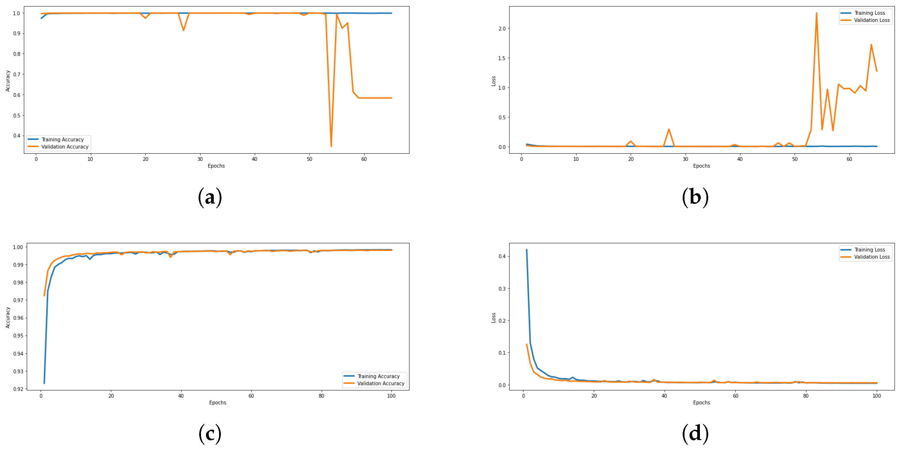
During training, we closely monitored overall metrics such accuracy, mIoU, F1 scores, and losses. However, due to the highly imbalanced nature of the dataset, these overall metrics or average metrics across all classes proved to be poor indicators of the model’s true performance. Specifically, the metrics were dominated by the more frequent classes, to the extent that the training and validation results did not align with the actual segmentation performance during inference. High training accuracy was primarily driven by the dominant classes, while the less frequent classes showed poorer results during inference. To better reflect the model’s performance and ensure consistency between training metrics and inference results, we decided to evaluate the metrics for each class individually. This approach allowed us to assess the model’s performance on specific classes during training, revealing that abundant classes in the dataset had better metrics, while the model struggled with less frequent classes. These class-specific metrics are more accurately reflected in the inference results. This prompted us to use the focal loss function during training, which effectively mitigated the class imbalance by giving more weight to the underrepresented classes. This adjustment resulted in more or less balanced performance across both frequent and less frequent classes. The training process was performed on a system equipped with an NVIDIA GeForce RTX 3090 Ti GPU (NVIDIA Corporation, Santa Clara, CA, USA), using a batch size of 10, with a learning rate of $6\times {10}^{-5}$.

4.3. Prediction and Model Inference

After successfully training the model, we evaluated its performance on a test set to predict segmentation masks for unseen TFT backplane images. This step validated the model’s ability to generalize and demonstrated its effectiveness in accurately segmenting high-resolution TFT images. Given the high segmentation accuracies, we then shifted our focus to optimizing inference speed, utilizing techniques such as image downscaling and data parallelism, all while ensuring that accuracy was not compromised.

4.3.1. Image Downscaling for Inference

When dealing with large images, it is often beneficial to resize them to expedite processing. In our task, large TFT backplane images, which can consist of 60 to over 100 $2048\times 2048$ patches, require significant processing time during segmentation, and we aim to minimize the segmentation time for these large images.

While we allow the model’s image processor to automatically resize all input images to $512\times 512$ during training, we found that during the inference, pre-resizing those $2048\times 2048$ patches externally to $512\times 512$ before passing them to the model significantly reduced inference time. This approach effectively skips part of the resizing overhead within the image processor, resulting in a reduction of inference time by a factor greater than 3, without affecting segmentation accuracy. By processing fewer large patches resized to $512\times 512$, rather than numerous smaller patches, the computational burden is significantly reduced. For example, a pre-processed TFT image with a resolution of $\mathrm{10,368}\times \mathrm{21,034}$ produces only 66 $2048\times 2048$ patches, compared to 881 $512\times 512$ patches. Processing the smaller number of resized larger patches is computationally much faster while still retaining the high segmentation accuracy of the model.

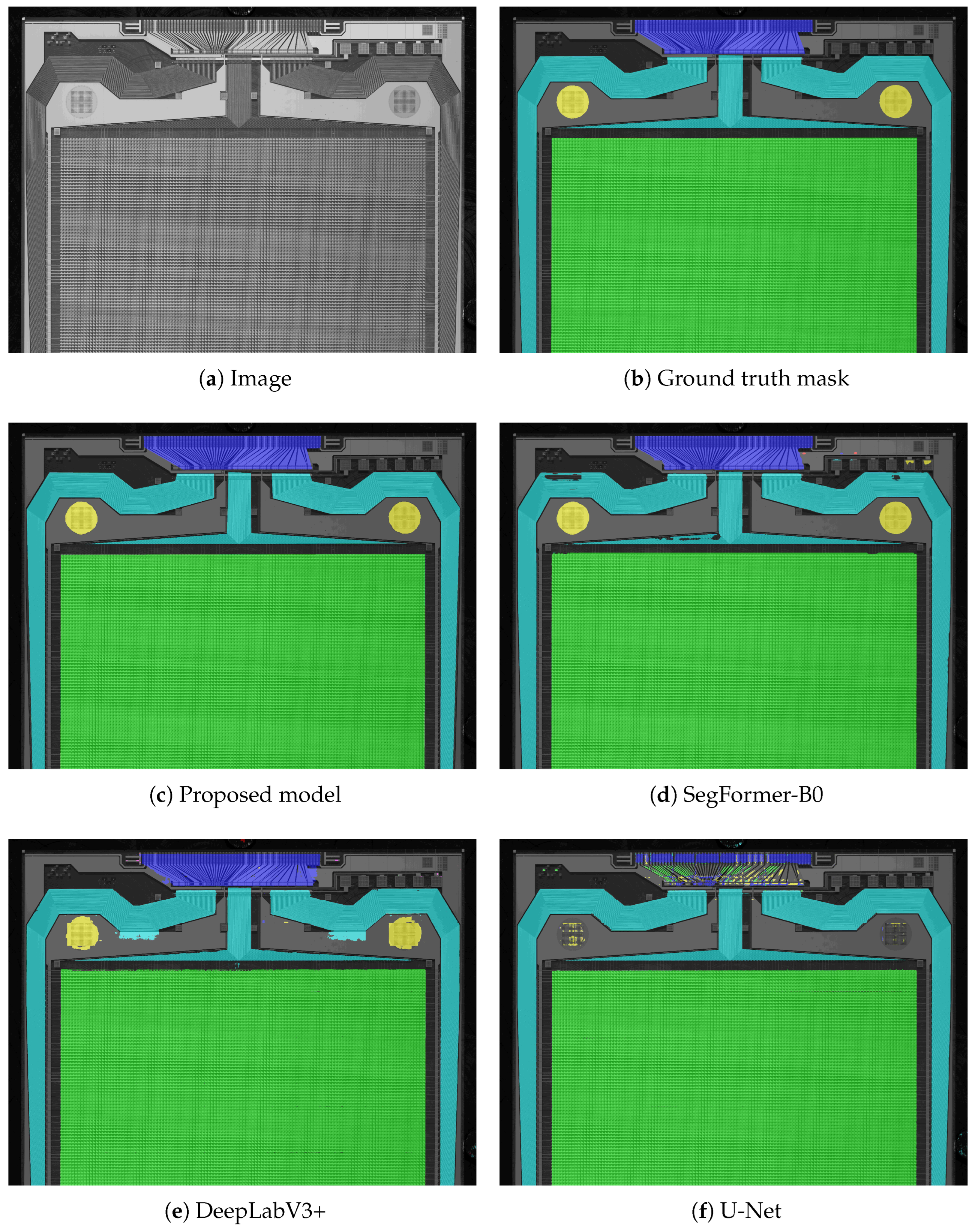
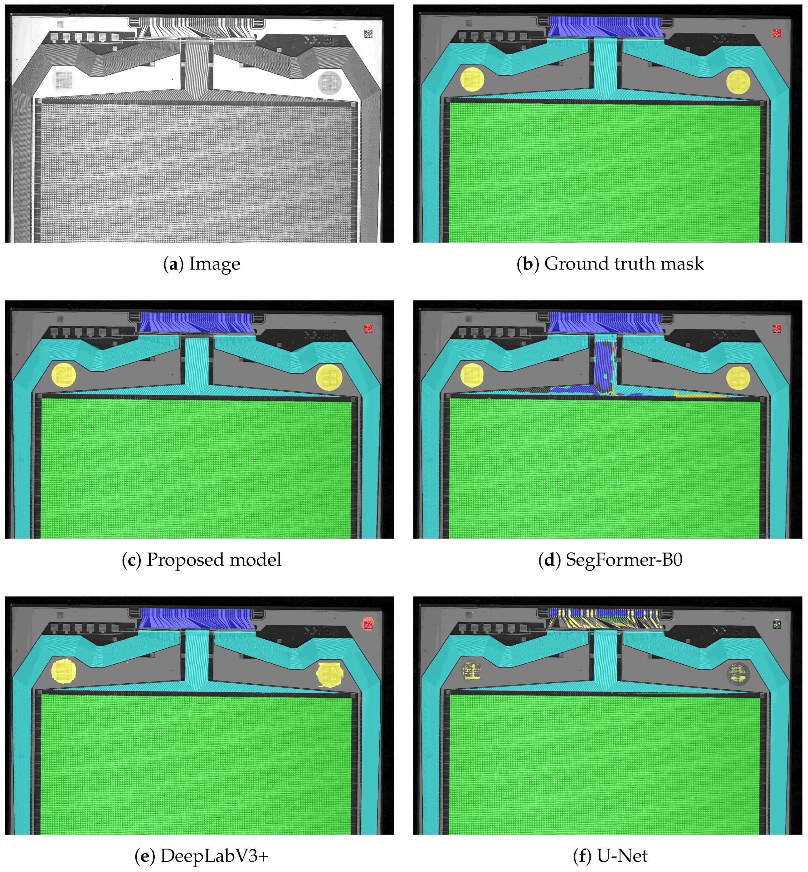
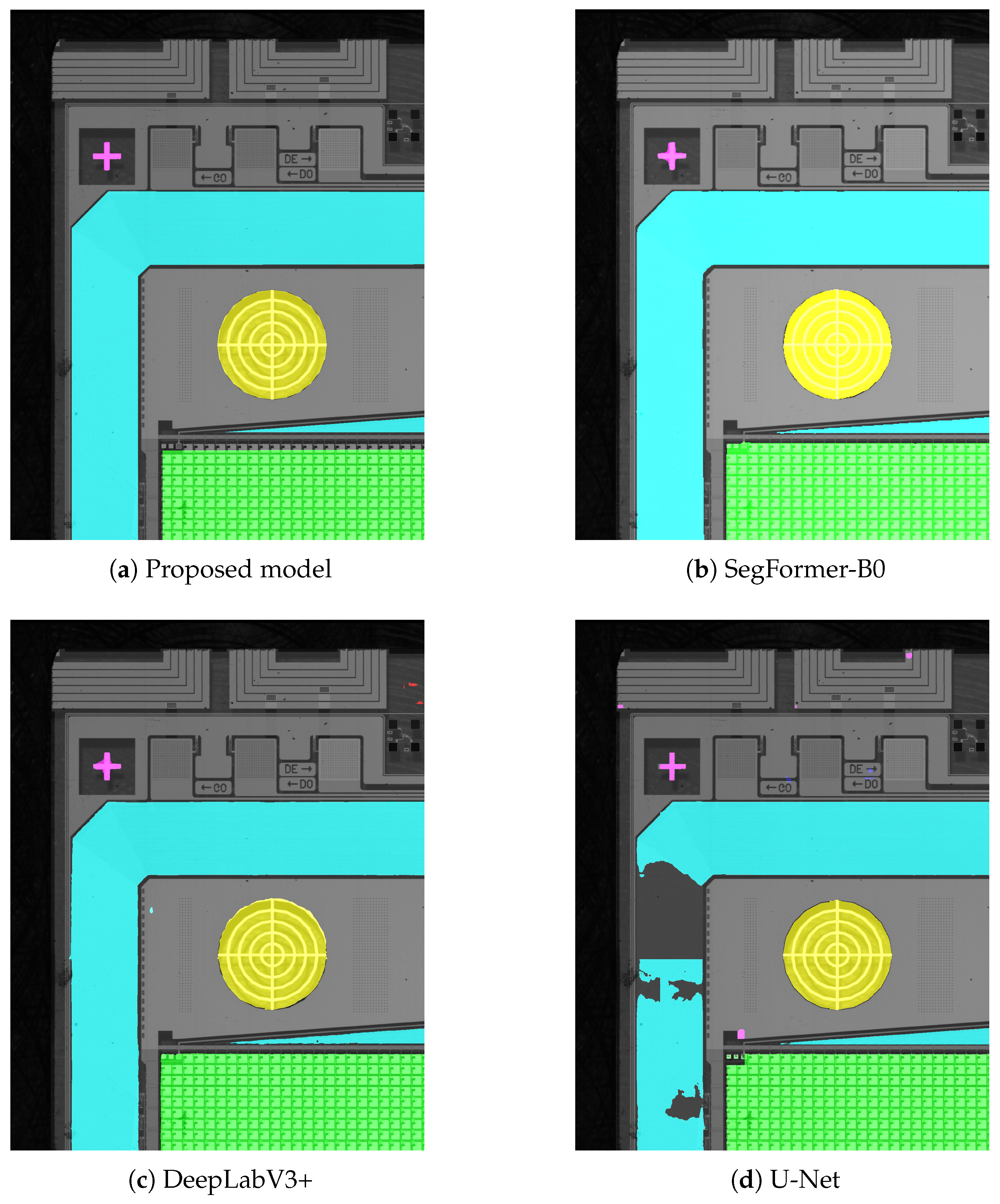
Our experiments revealed that the patch size used during training significantly impacts the model’s ability to generalize. TFT backplane images contain intricate patterns, as can be seen in Figure 7 and several variations, that challenge semantic segmentation models, especially when the patch sizes used in training and testing differ. When trained on $512\times 512$ patches, the model learns features and contextual information specific to that resolution, performing only well on test patches of the same size despite the use of data augmentation during training. Similarly, models trained on $1024\times 1024$ or $2048\times 2048$ patches achieve high accuracy when tested on patches matching their training resolution. This behavior suggests that, despite the image processor resizing all input images before passing them to the model, the learned features remain resolution-dependent, making it difficult for the model to generalize effectively across different patch sizes. This pattern was observed on all the models we trained on the dataset.

To address this limitation and ensure that the model generalizes across multiple patch sizes, we trained it on a hybrid dataset containing patches of varying resolutions ($512\times 512$, $1024\times 1024$, and $2048\times 2048$). Because the model’s image processor automatically resizes all inputs to $512\times 512$, the model can seamlessly process this hybrid dataset without additional adjustments. Training on patches of different resolutions increased the model’s multi-resolution feature learning, improving its generalization performance across patches of varying sizes during inference.

To ensure minimal information loss during downscaling while preserving high segmentation accuracy, we employed the INTER_AREA interpolation method from OpenCV [25] for resizing. This method, optimized for efficient downscaling, averages pixel areas to minimize artifacts such as moiré patterns and aliasing effects, which are common with simpler interpolation methods. After inference, the predicted segmentation masks are re-upscaled to the original $2048\times 2048$ resolution using bilinear or bicubic interpolation. This ensures that the reconstructed large masks match the original image size and maintain high segmentation quality.

4.3.2. Data Parallelism for Inference

To further reduce the inference time of large image segmentation tasks, we effectively used parallel computing. By dividing the image into patches and processing them independently, we harnessed the parallel processing capabilities of both the CPU and the GPU to achieve substantial speedup. In the inference process shown in Figure 8, we found that part of the bottleneck in the task flow lies in the sequential feeding of image patches to the model. To overcome this limitation, we parallelize this step, allowing multiple patches to be sent simultaneously to the model for prediction. This allows the GPU, which inherently supports parallel processing, to work on multiple patches concurrently, resulting in a significant reduction in overall inference time.

Our approach aligns with Gustafson’s law (5) [26], which offers insights into the potential speed-up achievable through parallelization.

$$S=P+N(1-P)$$

(5)

where $\mathrm{P}$ is the portion of the code that is parallelizable, $\mathrm{N}$ the number of processors, and $\mathrm{S}$ is the speedup gained through parallelization.

We estimated the anticipated speedup gained from parallelizing the patch feeding process on a computer equipped with an i5-12400F CPU boasting 6 cores. The results underscore the tangible improvement achieved through parallelization of part of the segmentation process. According to Gustafson’s law, we anticipated further reduction in inference time on systems with more than 6 processors, and it was confirmed when we tested the model on the 24-core computer used for training.

5. Results

5.1. Accuracy and Inference Speed

The results of our project demonstrate the exceptional effectiveness and efficiency of using deep learning models for the semantic segmentation of high-resolution images in the semiconductor industry. In addition to achieving high segmentation accuracy, the proposed model shows how incorporating dilated convolution for feature extraction in the encoder of a transformer model enhances the sharpness of the predicted segmentation masks. The accuracy reaches as high as $98\%$ for some classes on our dataset, even with a limited amount of training data and a short training period. Figure 9 shows results from the proposed model, where it is clear that the edges are improved compared to the results of SegFormer, which are shown in Figure 5.

By replacing two transformer blocks by atrous convolutions, the number of parameters in the proposed model is 3.08 million compared to 3.8 million parameters for SegFormer-B0. Although the number of parameters and FLOPS are comparable—9.06 GFLOPS for the proposed model and 10.35 GFLOPS for SegFormer-B0 on $512\times 512$ images—we achieved a substantial reduction in processing time through the incorporation of image downscaling and parallel processing during inference.

This optimization resulted in over four times faster inference compared to SegFormer, which is the model closest to it in architecture. The use of image downscaling and parallel processing in SegFormer also improves its inference speed. On a system equipped with a 12th Gen Intel^® Core^TM i5-12400F processor (Intel Corporation, Santa Clara, CA, USA) and an NVIDIA GeForce RTX 3050 GPU (NVIDIA Corporation, Santa Clara, CA, USA), parallel processing led to a significant decrease in inference time as seen in

Table 1. Comparing the Inference Time for SegFormer-B0 and the proposed model under data parallelism.

	SegFormer	Proposed Model
Single Processor Inference Time (s)	~42	~9
Six Processors Inference Time (s)	~15	~3

. When tested on the 24-core i9-13900F computer used for the model training, the inference time was further reduced to less than a second as predicted by the parallelization law.

5.2. Comparison with Other Models

We conducted a comparative analysis of the proposed model against SegFormer, DeepLabV3+, and U-Net models by training each on the same dataset and evaluating their performance across various metrics. Despite training DeepLabV3+ and U-Net for more epochs, no significant improvement in overall performance metrics was observed, even with the extended training. However, DeepLabV3+ and U-Net did show better-defined edges in their segmentation maps compared to SegFormer, despite the presence of some false positives in the prediction given the characteristics of the images, that make it very hard for models to effectively learn during training. Figure 10 and Figure 11 present visual comparisons of segmentation masks predicted by the four models. While U-Net and DeepLabV3+ generate more accurate edges than SegFormer-B0, their boundary quality still lags behind the proposed model.

Our class-specific metrics confirm that the models perform better on the dominant classes compared to under-represented classes. The proposed model has training metrics on par with SegFormer and the boundaries of the segmentation masks obtained using the proposed model are indeed clearer and sharper compared to those obtained using SegFormer. This indicates that our approach, which incorporates dilated convolution for feature extraction, does improve local feature extraction, especially for less frequent classes in the dataset. In the case of U-Net, all three models (the proposed model, SegFormer, and DeepLabV3+) outperform it in every metric, despite U-Net also demonstrating strong performance. We believe one of the reasons for this is the use of pre-trained weights and biases in SegFormer and DeepLabV3+. The complexity of the images can also explain why the convolution-based models display a higher number of false positives in the segmentation masks. Figure 12 shows a part of a TFT backplane segmented used the proposed model with the regions of interest in our task indicated.

Table 2. Class accuracies.

Model	AA	LF	QR	AP	CA	IC
SegFormer-B0	0.99	0.99	0.93	0.90	0.95	0.97
DeepLabV3+	0.95	0.95	0.85	0.83	0.92	0.93
U-Net	0.90	0.91	0.56	0.63	0.75	0.88
Proposed model	0.99	0.99	0.97	0.95	0.96	0.98

,

Table 3. Class IoUs.

Model	AA	LF	QR	AP	CA	IC
SegFormer-B0	0.97	0.96	0.91	0.88	0.90	0.94
DeepLabV3+	0.93	0.92	0.82	0.87	0.90	0.91
U-Net	0.91	0.87	0.79	0.75	0.81	0.83
Proposed model	0.98	0.96	0.96	0.94	0.93	0.96

and

Table 4. Class F1 scores.

Model	AA	LF	QR	AP	CA	IC
SegFormer-B0	0.98	0.97	0.92	0.85	0.93	0.97
DeepLabV3+	0.94	0.93	0.88	0.85	0.90	0.92
U-Net	0.92	0.91	0.69	0.76	0.82	0.88
Proposed model	0.98	0.98	0.97	0.90	0.96	0.97

compare the accuracies, intersection over union (IoU), and F1 scores of the models across the classes representing those regions of interest.

For the AA, LF, and IC classes, the accuracies for SegFormer are close to those obtained with the proposed model. These classes occupy larger segments in the raw images used for training and testing, and being part of the dominant classes in the dataset, SegFormer has no significant issues segmenting them. As a result, SegFormer’s accuracy for these classes is consistently high. However, it should be noted that high accuracy does not necessarily translate into well-defined contours. Even in regions where the accuracy reaches $99\%$, the edges of the segmentation maps remain poorly defined, with a noticeable lack of sharpness. This is where the proposed model aims to improve—not just maintaining the high accuracy of SegFormer for these dominant classes, but also improving the accuracy of the other less dominant classes, while enhancing the local feature extraction to provide better edge and contour definition.

Figure 11 presents cropped sections of the segmentation masks predicted by the four models, overlaid on the original images. These results show that models such as U-Net still perform poorly, even on dominant classes. They also reveal notable differences in boundary quality: some models produce clearly defined segmentation edges, while others exhibit fragmented or inconsistent mask structures. In all examples, the proposed model demonstrates superior performance compared to SegFormer-B0 and DeepLabV3+. Figure 13 further compares the four models on TFT backplane images with varying designs and textures. These additional results highlight the generalization capability of the proposed model, which consistently outperforms SegFormer-B0, DeepLabV3+, and U-Net across different image types and patterns.

Although SegFormer attains high training accuracy across all six classes in our dataset and performs well on many test images, its performance degrades considerably on more challenging and diverse test images as seen in Figure A5 of Appendix A. This decline indicates overfitting, where the model learns dataset-specific patterns rather than generalizable features. The high representational capacity of the transformer encoder, while effective for capturing complex structures, can also lead to reliance on training-set biases, such as specific textures or class distribution characteristics.

In contrast, the proposed model, in which two of SegFormer’s transformer blocks are replaced with atrous convolutions, demonstrates improved generalization on difficult test cases. This architectural adjustment introduces a beneficial inductive bias that mitigates overfitting. Training dynamics further support this observation: SegFormer’s validation accuracy and loss begin to deteriorate after approximately 50 epochs, despite continued improvement on the training set (Figure 14a,b), which is a typical indication of reduced generalization capability. Conversely, the proposed model maintains consistent improvements in both accuracy and loss beyond 100 epochs (Figure 14c,d), suggesting a more stable optimization process and stronger generalization.

Given the absence of validation improvement and the high computational cost, SegFormer training was terminated after 65 epochs. Additional qualitative comparisons among the proposed model, SegFormer, DeepLabV3+, and U-Net are provided in Appendix A.

5.3. Integration to the TFT-DRE Application

The model effectively automates the segmentation of regions of interest (ROIs) in images loaded into the AOI system. Figure 15 shows examples of the ROIs automatically detected by the model after integration into the system. These selected regions have well-defined and sharp boundaries, which are crucial for accurately identifying the points of interest (POIs).

The effectiveness of the post-processing techniques is demonstrated in Figure 16. As shown in Figure 16a, the model’s initial predictions contain several inaccuracies, including false positives and false negatives. After post-processing is applied, especially steps 1 through 5 in Algorithm 1, the images in Figure 16b show that these errors have been corrected, with the segmentation maps now accurately representing the ROIs. The RDP used in step 7 of the algorithm simplifies the contours, making them easier to handle and edit. This simplification process also refines the edges of the contours, ensuring they more accurately match the ROI for precise identification.

Table 5. Effects of the RDP algorithm on the contours.

Contours	Contours Points (Before RDP)	Contour Points (After RDP)
AA	4999	8
CA	1403	425
IC	874	10
AP	202	153
LF	6996	41
QR	25	14

compares the number of contour points before and after applying the RDP algorithm. For example, large contours, such as those representing the AA and LF regions, which initially appeared complex with many vertices, are significantly simplified into polygons with far fewer points. This simplification enhances the efficiency of the inspection process by reducing the amount of data needed to represent each ROI. For instance, the number of points required to represent the AA ROI drops from 4999 to just 8, which allows the system to track and process the coordinates of the ROIs more efficiently. This is especially important for accurate defect localization and efficient inspection. The effect of the RDP algorithm is less significant on smaller contours, as they are simplified with a higher tolerance value ($ϵ$), resulting in a more modest reduction in their number of vertices.

Once the ROIs are post-processed, they are represented as polygons with clearly defined vertices, as shown for the CA class (yellow) in Figure 15b. Users can click and drag the vertices or delete them to reshape the polygons, ensuring better alignment with the areas of interest if there is slight misalignment. The TFT-DRE application also allows users to add new vertices by clicking on the edges of the polygons, providing additional flexibility when reshaping the contours. While the need for such adjustments is rare, these functionalities were incorporated to enhance the application’s usability and ensure that it can handle edge cases when necessary. The coordinates of the vertices and POIs are then saved and passed to the next stage, where the AOI system uses the POIs as reference points to inspect each ROI. This ensures precise defect detection and facilitates the collection of relevant inspection data for each ROI.

Given that the AOI system conducts defect detection on smaller ROIs, accurately pinpointing the exact location of defects in the larger image can be a challenge. However, by saving both the POI coordinates and the contours of the ROIs, we can easily track and localize defects across the entire image, even when defects appear in different regions. Locating defects in the larger image is critical, as it provides valuable feedback to engineers, helping them identify the root cause of recurring defects. For example, if multiple defects consistently appear in the same location within the larger image, it suggests that a specific part of the manufacturing process may be responsible. This approach reduces the time spent on random troubleshooting and helps streamline the corrective process.

6. Conclusions

This study has successfully demonstrated that deep learning can be effectively applied to semantic segmentation in semiconductor optical inspection, achieving state-of-the-art performance. The proposed model highlighted the advantage of combining convolutions and transformers for efficient extraction of both fine-grained features and global context in the feature map. This approach not only achieves high accuracy in identifying and classifying pixels in complex high-resolution images, but also maintains practical inference times, which is a critical factor for real-world industrial applications. Our research outcomes underscore the potential of deep learning to improve region segmentation in automated optical defect inspection across various semiconductor manufacturing sectors, offering more precise and efficient segmentation capabilities. The successful application of this model to TFT backplanes paves the way for future advancements in quality control processes. This can significantly contribute to increased production efficiency and product quality assurance in high-resolution semiconductor manufacturing.

Future research will focus on extending the segmentation approach developed in this study to tackle other semiconductor defect detection challenges, particularly in applications such as lens-less diffraction imaging and other advanced semiconductor inspection tasks. Additionally, we aim to further enhance the scalability and robustness of the model to handle even more complex and varied industrial inspection scenarios.