Abstract
The use of low-resolution analog-to-digital converters (ADCs) in receivers has emerged as an effective solution for reducing power consumption in millimeter-wave (mmWave) massive multiple-input–multiple-output (MIMO) systems. However, low-resolution ADCs also pose significant challenges for channel estimation. To address this issue, we propose a joint uplink/downlink (UL/DL) channel estimation algorithm that utilizes the spatial reciprocity of frequency division duplex (FDD) to improve the estimation of quantized UL channels. Quantified UL/DL channels are concentrated at the BS for joint estimation. This estimation problem is regarded as a compressed sensing problem with finite bits, which has led to the development of expectation-maximization-based quantitative generalized approximate messaging (EM-QGAMP) algorithms. In the expected step, QGAMP is used for posterior estimation of sparse channel coefficients, and the block maximization minimization (MM) algorithm is introduced in the maximization step to improve the estimation accuracy. Finally, simulation results verified the robustness of the proposed EM-QGAMP algorithm, and the proposed algorithm’s NMSE (normalized mean squared error) outperforms traditional methods by over 90% and recent state-of-the-art techniques by 30%.
1. Introduction
Massive multiple-input–multiple-output (MIMO) technology is regarded as a key component of 5G wireless communication systems. By utilizing large-scale antenna arrays, it significantly increases both communication capacity and energy efficiency [1]. This enables the base station (BS) to perform multi-user beamforming with narrower beams, reducing interference and improving service quality for multiple users simultaneously [2]. However, to fully achieve these benefits, accurate channel state information (CSI) is essential for tasks, such as precoding and signal detection.
For downlink (DL) transmission, it is necessary to timely and accurately acquire the CSI at the BS for precoding. In frequency division duplex (FDD) systems, this becomes especially challenging since channel reciprocity is no longer valid—uplink (UL) and DL transmissions operate at different frequencies. To estimate DL CSI, the BS must conduct DL training, after which the user estimates and quantizes the CSI and feeds it back to the BS. However, with traditional channel estimation and feedback methods, the overhead for DL training and feedback increases linearly with the number of antennas at the BS, which is unaffordable. Additionally, the complex wireless environment and high-dimensional signals further escalate the difficulty of DL channel estimation. As a result, current research is focused on exploring approaches to achieve accurate DL channel estimation while minimizing the training and feedback overhead.
Another major challenge is the use of low-resolution analog-to-digital converters (ADCs), which renders traditional channel estimation methods that do not account for hardware impairments no longer applicable. Specifically, due to the exponential increase in costs associated with higher bit resolutions of ADCs [3], BSs typically employ low-resolution ADCs, such as 1 to 4 bits, to reduce power consumption and hardware costs in massive MIMO systems. Ref. [4] further emphasized that, with the enhancement of an ADC’s resolution, its theoretical minimum energy consumption also increases. However, the actual energy usage of ADCs often escalates at a faster pace, approaching exponential growth, which exceeds the thermal constraints caused by architectural intricacies and other limitations, particularly in the high-resolution domain. The application of such low-resolution ADCs leads to a decrease in signal quantization accuracy, which seriously affects the amplitude and phase information in the uplink (UL) signal received by the BS and may potentially lead to considerable loss or distortion [5]. In addition, the angle information may also be biased [6]. In [7], the pilot sequence duration must be significantly extended (for example, about 50 times the number of users) to ensure adequate beamforming effectiveness for the MIMO system with 1-bit ADCs. Hence, an efficient approach for estimating DL channels specific to low-resolution ADC systems is critically required.
To overcome the above challenges, many efficient channel estimation approaches with low-resolution ADCs [8,9,10,11,12,13,14,15] have been proposed. Ref. [8] proposed an angle domain channel estimation scheme with one-bit ADCs. In [9], an expectation maximization-propagation (EM-EP) algorithm was used to obtain the maximum likelihood (ML) channel estimation based on the quantized output. Ref. [10] designed ML-based methods for UL channel estimation, but their algorithms are computationally intensive, which prevents their practical application. In [11], the authors adopted a one-bit threshold quantization strategy that changes over time and proposed a new method for UL channel estimation in the angle domain. In [12], the authors proposed generalized approximate message passing (GAMP)-based approaches for the estimation of the UL channel. Ref. [13] proposed a two-stage algorithm combining simultaneous orthogonal matching pursuit (SOMP) and space-alternating generalized expectation maximization (SAGE) for user position and orientation estimation in 5G millimeter-wave MIMO systems, achieving high-accuracy channel parameter estimation through sparse representation and iterative optimization. An efficient DL model known as bidirectional long-short-term memory (BiLSTM) was proposed in [14] for channel estimation in FDD systems and [15] used the special row–column sparse characteristics of the channel matrix and proposed a row-structured sparsity based on the orthogonal matching pursuit algorithm (RS-OMP).
However, only UL channel estimation in the time division duplex (TDD) system is considered in previous research on low-resolution ADC channel estimation [10,11,12]. The reason for this focus is the high channel reciprocity between UL and DL channels in TDD systems, which allows the DL CSI to be inferred from UL CSI with minimal effort. Moreover, obtaining the UL CSI is relatively straightforward, as the training overhead is only proportional to the number of users. In FDD systems, the situation becomes fundamentally different, where the UL and DL channels are no longer reciprocal. Due to the lack of reciprocity, accurate DL channel estimation suffers from serious obstacles because it requires the users to provide explicit feedback, resulting in prohibitively training and feedback overhead. Existing methods that attempt to address DL channel estimation either fail to scale effectively in massive MIMO scenarios or require substantial additional resources for accurate CSI acquisition. For example, the complexity of ML algorithms increases exponentially with the number of paths, and the SOMP-SAGE algorithm heavily relies on the estimation accuracy provided by the SOMP stage and the sparsity of the channel, initial estimation errors, and cross-interference caused by overlapping paths can significantly affect the final performance. But in FDD systems, the UL and DL channels exhibit partial reciprocity due to their shared scattering environment, resulting in consistent geometric structures, including propagation delay, angle of arrival/departure (AoA/AoD), and multipath cluster distribution within similar frequency bands. Therefore, large-scale parameters (LSPs), such as the spatial covariance matrix and channel subspace, estimated from UL channel measurements, can be exploited to derive corresponding DL channel parameters [16]. Consequently, the estimation of both the UL and DL channels in FDD massive MIMO systems with low-resolution ADCs has their own difficulties and challenges that require resolution.
Therefore, in this paper, we consider a massive MIMO system with low-resolution ADCs in FDD mode for the joint estimation of the UL and DL channels. With spatial reciprocity, UL-aided DL channel estimation has been proposed in many previous works [17,18,19]. In practical deployments, Huawei’s Massive MIMO product line employs joint estimation techniques based on spatial reciprocity in FDD bands. This approach acquires spatial information through the estimation of the UL channel and applies this information to the DL beamforming. In order to take advantage of the sparsity of massive MIMO channels in the angular-delay domain, it is necessary to use adjustable sampling grids to cover the angular domain and the delay domain, respectively. After discrete sampling, the channel is converted into a sparse representation in the angular-delay domain. Then, the compressed sensing (CS) method is used to estimate the UL/DL angular-delay domain channel. Then, using a Bernoulli–Gaussian mixture (BG) distribution to model the sparsity of the channel coefficients, and solve the sparse channel recovery problem based on CS. Considering the impact caused by the compression and recovery process, the DL signal received by the BS will have additional noise, which can be assumed to follow the Gaussian distribution with zero mean and unknown variance. The main contributions of this paper are summarized as follows:
- A joint estimation framework that combines the UL and DL transmissions: The UL/DL channels have partial reciprocity. Therefore, a joint estimation framework that combines the UL and DL is considered. Utilizing UL channel information to assist DL channel estimation offers significant advantages. During the UL training phase, the user equipment (UE) sends training pilots to the BS, and the BS receives UL signals. Since the base station is equipped with low-resolution ADCs, the UL received signal will be affected by the coarse quantization effect. In the DL training stage, the BS will send training pilots to the UE, and then the UE will compress the DL signal and digitally send it back to the BS. Meanwhile, the error caused by quantization on UL channel parameter estimation can be reduced by using the feedback DL signal.
- An angular-delay domain parameterized estimation method: In contrast to traditional channel estimation methods for low-resolution ADCs, we propose an angle-delay domain parameterized channel estimation in a grid-based approach instead of full channel estimation, which significantly reduces the number of unknown parameters requiring estimation. This method shifts the focus to parameterizing the channel in the angle-delay domain, and then the angular and delay parameters are discretized onto a grid, allowing for a systematic and organized parameterization. This not only reduces the dimensionality of the estimation problem but also allows for more targeted estimation of key channel characteristics, leading to improved accuracy compared to full channel estimation.
- A novel algorithm based on the EM framework: An EM-based quantized GAMP algorithm (EM-QGAMP) is proposed for joint parameters learning and sparse signal recovery. The EM algorithm can effectively solve the parameter estimation problem with unknown variables (channel gain coefficient), and the QGAMP algorithm can obtain the posterior estimate of unknown variables in the expectation step. Compared with the existing algorithm, it can achieve better performance improvement under the condition of low-resolution quantization.
The proposed scheme for the joint estimation of the UL/DL channels has the following advantages: First, the channel estimation process can be completed on BS. With the powerful data processing capabilities of the BS, the energy of the UE can be effectively saved. Second, the dimension of the DL received signal is generally much smaller than that of the channel dimension in massive MIMO systems, so the feedback overhead can be significantly reduced. Third, unlike deep learning neural networks [20,21], our algorithm does not require extensive training under specific system configurations, and can adapt to changes in system parameters in real time. Relying on partial spatial reciprocity and adjustable grid parameterization, our method achieves excellent performance without data collection and model retraining.
2. System Model
2.1. Channel Model
Consider a flat fading massive MIMO system in FDD mode, where the BS is equipped with a uniform linear array (ULA) of antennas to serve single UE with antennas. The DL and UL channel matrix is given by
where L denotes the number of channel paths. For the sake of clarity, without ambiguity, the indicators of the UL and DL are replaced with * hereinafter. In (1) and (2), , , , stands for the channel coefficient, the angle of arrival/departure (AoA/AoD) from BS, and the angles of arrival/departure from user and delay of the l-th path, Moreover, the steering vectors of the user and BS is given by
where d stands for the separation distance between the antennas, is the wavelength of UL/DL. For broadband communication, orthogonal frequency division multiplexing (OFDM) modulation with N subcarriers will be used, and B is the signal bandwidth. is defined as the subcarrier spacing. Then, the channel matrix on the n-th subcarrier is denoted by . In BS, G OFDM symbols are transmitted sequentially, where the g-th transmitted symbol for the UL is for each subcarrier and . Similarly, the counterpart for DL is . These symbols are transformed to the time domain using an N-point IFFT. Before converting the baseband signals to RF signals, a cyclic prefix (CP) of length is added, where is the sampling period, and is the length of CP within the sampling periods. Assuming that the channel remains unchanged throughout the entire transmission of G symbols, the UL and DL channel matrices in subcarrier n are expressed as
herein, ∘ is the Hadamard product of and . We denote , , where we let and denote the BS and UE’s array response vectors of the l-th path and on subcarrier n, respectively. and . The true AoAs/AoDs of the BS and UE as well as the delay are denoted as , respectively. Denoting the UL channel across all subcarriers as , while the structure of DL channel is similar to the UL channel.
After CP removal and FFT, the signal received on the subcarrier n and the symbol g is given by
where denotes a Gaussian noise vector with zero mean and variance per real dimension, and , . Stacking the observation with g, we can get , where and .
Stacking the observation along n, we have
where , ,
, and .
2.2. Sparse Representation
To take advantage of the sparsity of the channel in the spatial domain, a fixed and dense grid is typically used for channel sparse representation. Define a fixed grid with M sampling points that evenly cover the angle and delay domains. As such, , and . The values of , and uniformly cover the range of , and , with the grid count for each range defined as , , and . Setting enables the grid encompass all possible combinations of AoA, AoD, and delay.
If the grid is fine enough that all the true AoDs/AoAs and delays lie on the grid, then the grid mismatch is negligible [22]. However, this requires very large , , and to achieve this effect, resulting in a high computational complexity of the algorithm. In order to address the mismatch and complexity inherent in using a fixed mesh, we opt for an adjustable grid where the grid parameters are adjustable rather than fixed. In this case, as long as the number M is larger than the number of paths L, there exists a set of unknown grid parameters that enables an accurate representation of the channel matrix. For instance, the DL channel matrix is given by
where , , and we represent . is a sparse vector whose non-zero elements correspond to the true channel coefficients. With a similar structure, such sparse representation can also be applied to the UL channel matrix. And the specific formula for UL is omitted to avoid redundancy. With the help of the adjustable grid, the signal received on subcarrier n and transmission g can be rewritten as . By stacking the observations first along g and then along n, we have
where , , and .
2.3. Joint UL/DL Received Signal
Considering an FDD massive MIMO system, the BS is equipped with low-resolution ADCs and the UE is equipped with perfect ADCs/DACs, as shown in Figure 1.
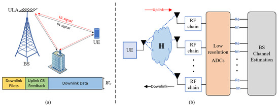
Figure 1.
An FDD massive system model with low-resolution ADCs at the BS. (a) The typical pilot transmission and CSI feedback mechanism in FDD mode; (b) The BS equipped with low-resolution ADCs.
The UL signal received at the BS is transmitted to the baseband through low-resolution ADCs, which can be expressed as
where is the uplink noise, and is the quantization operation of DACs. When the quantization bit is b, for scalar input y, the quantization output is
where the quantization thresholds , for , and , , , is the stepsize.
The feedback DL signal received by the BS can be expressed as
where is the noise caused by compression and quantization in the signal feedback process, and is the identity matrix. is the total noise of the feedback signal received by the BS.
In the DL channel estimation process, the received DL signals are compressed and quantized, and then fed back into the BS. Considering the compression and quantization errors in the feedback process, the noise can be modeled as an additive noise with a Gaussian distribution with zero mean and unknown variance. The BS will perform joint UL/DL channel estimation. This feedback scheme has been proposed in previous works [16,23]. In this paper, it does not consider the specific feedback process (such as UE directly feedback the received signals or estimated channel parameters to rebuild the DL signals on the BS) and the effect of low-resolution ADCs on the feedback signals. The UE feeds the compressed and quantized signal back to the BS digitally. As long as the number of bits per symbol of the feedback signal does not exceed the channel capacity of ADC, it can pass through the ADC without loss and then be recovered at the BS.
This feedback method offers several advantages: first, the channel estimation process can be completed on the BS, thereby conserving energy on the UE. Second, the dimension of the received signal is much smaller than the dimension of the channel itself in massive MIMO systems, which also reduces the feedback costs. The BS can perform joint UL/DL channel estimation within the channel statistical coherence time [24].
When the fixed grid is known, the model is a linear model. The recovery of can be formulated as a least absolute shrinkage and selection operator (LASSO) problem that is convex and can be guaranteed to converge to global optimality. However, with the AoD, AoA, and delay grid as tunable variables, the measurement matrix in (11) and (13) will contain unknown grid parameters , and . Thus, (11) and (13) are no longer standard CS models with known measurement matrices. The problems of learning grid parameters and recovering sparse channels cannot be solved by traditional orthogonal matching pursuit (OMP) algorithms [25,26] or LASSO [27]. In order to recover and learn unknown grid parameters, an EM-based QGAMP framework is adopted, as described in the following section.
3. Problem Formulation
3.1. Bernoulli–Gaussian Prior
In massive MIMO systems, the BS is commonly assumed to be mounted at a height, which results in a limited number of scattering clusters. Moreover, the sub-paths associated with each scattering cluster tend to concentrate in a small range, which results in concentrating within a narrow range around a few positions. In this case, possesses an unknown block-sparse structure. Therefore, it is necessary to adopt the widely used Bernoulli–Gaussian mixture (GM) distribution to describe the sparsity of . Assume that each item of sparse signal is i.i.d. [28].
where is the Dirac function, is the probability of taking non-zero value, is the Gaussian mixture weight, and is the mean and variance of the i-th Gaussian component. In this case, the parameter set is
where is the number of GM distribution elements.
3.2. Problem Statement
As mentioned earlier, the true angles and delay are not always aligned with the predetermined sampling grids, resulting in an inevitable discrepancy between the sampling grid and the actual values. This misalignment may manifest in a substantial number of non-zero entries within the associated sparse vectors, which can significantly impede the effectiveness of the sparse recovery methods. To address this issue, this paper considers , and as unknown continuous parameters and explores a joint problem of parameter learning and sparse channel recovery.
Since is a sparse vector, we can consider a sparse channel recovery method based on CS to estimate through Equations (11) and (13). Given the value of , and , can be derived by using the Bayesian criterion, as shown in the following equation
where , denotes the k-th row of .
Given the posterior distribution, the estimation of can be obtained by computing the posterior mean.
The notation denotes the integration over all variables in except for . In (18), high-dimensional integration is involved, and the exact estimate of in (17) is computationally prohibitive. Nevertheless, by using loopy belief propagation, the GAMP algorithm serves as a tractable way to approximate these marginal posterior distributions and posterior means.
On the other hand, for the unknown parameter sets, the ML algorithm can be used to solve , where , and , , is the noise accuracy. To maintain generality, it is modeled as a gamma prior , which involves two parameters and . By setting them to be sufficiently small values, it can be ensured that the noise prior does not contain information.
For the parameter estimation problem containing unknown variables, the solution is that of using the EM algorithm and treating as a hidden variable. In the E-step, the mean and variance of are obtained by using the GAMP algorithm. Then, in the M-step, the most likely values of the remaining parameters are estimated by using maximum likelihood estimation.
4. Proposed Algorithm
4.1. Posterior Approximation via GAMP
In the EM framework, it requires an accurate posterior distribution to iteratively estimate the parameters where . However, it is difficult to carry out theoretical analysis under the BG prior. Therefore, we employ GAMP to compute the corresponding approximate posterior distribution. In the GAMP algorithm, we consider the hyperparameters in the t-th iteration to be fixed, and will be updated later based on the EM framework.
GAMP models the relationship between the k-th observed output and the corresponding noiseless output . Using the conditional probability density function (pdf) , the marginal posterior distributions of and at the t-th iteration are approximated by
For simplicity, the notation * and the iteration count t are omitted. Similarly to [28], we use the GAMP and EM to update the variables of interest. Specifically, in each iteration, the variables are updated by GAMP, where are the estimations of the mean and variance of , and correspond to the mean and variance of the marginal posterior distribution of . is updated by maximizing the marginal posterior distribution through the EM method. Herein, the summaries about the detailed steps of the proposed algorithm are shown in Algorithm 1.
| Algorithm 1 GAMP-based few bits recovery algorithm. |
Input: , , , , . Output: , . 1: Initialize: , , . 2: repeat 3: Update using (21) and (22). 4: 5: 6: Update using (33) and (34). 7: Update using (35) and (36). 8: Update using (37) and (38). 9: Update through EM. 10: . 11: until . |
For line 3 of Algorithm 1, compute by
The DL signal processing can be conducted using the conventional GAMP algorithm. For UL signals, Algorithm 1 differs from the traditional GAMP due to the quantization effect introduced by the ADCs, which is mainly reflected in lines 4 and 5, where the quantization operations are executed. Consequently, this paper will focus on explaining the derivation process for lines 4 and 5 of Algorithm 1, as it is related to the estimation of UL signals.
For the case of quantized outputs, we have , where is the indicator function, , , and represent the lower and upper limits of the range indicated by the quantized output when a particular quantizer is applied. Under the AWGN assumption, the conditional pdf is
where we denote and , when and .
Plugging (23) into (19) and then substituting (19) into line 5 of Algorithm 1 and omit the superscript t in the following derivations. We have
within the EM-QGAMP framework, the posterior variance is approximated as
where is the prior variance, and is the correction term introduced due to the quantization effect. The correction term is expressed as
where is the cumulative distribution function of the standard normal distribution and is the probability density function of the standard normal distribution.
as obtained from line 5 of Algorithm 1:
the posterior mean is defined as the expectation of under the conditional posterior distribution:
the likelihood accounts for the quantization process:
under additive Gaussian noise with variance , this models the probability of being mapped into the quantization bin . Then, we performed the same operation in line 5 of Algorithm 1, which produces
the real and imaginary parts are quantized separately, and each complex-valued channel can be decoupled into two real-valued channels. Equations (25) and (32) are the estimators only for the real part. For the ease of notation, we abused and in (25) and (32) to denote and , respectively. Similarly, an estimator for the imaginary part can be obtained as in (25) and (32), while and b should be replaced by and , respectively.
For line 6, update the state variables through Equations (21), (22), (24), and (29):
For lines 7 and 8 (sparse coefficient updates), update , which are intermediate variables used to refine the estimates of the sparse signal coefficients and compute the updated variance and mean for each sparse coefficient:
4.2. Hyperparameter Learning via MM
In this subsection, we learn the hyperparameters within the EM framework. It is noted that the derivation of the GM parameters is an existing method, the details of which can be obtained from [28]. Therefore, this paper focuses on the derivation of the rest parameters .
We treat as hidden variables and iteratively maximize the likelihood function , where . However, it is challenging to directly maximize the objective function due to the lack of a closed-form expression. To make the problem tractable, in the M-step, we gradually set about building a substitute function to approximate the objective function. This substitute function was designed to simplify the optimization process for each variable. Specifically, let denote the surrogate function and is a fixed point, around which the surrogate function is established. The surrogate function must satisfy the following properties,
let denote the optimization variables at the beginning of the t-th iteration. Then, in the t-th iteration of the block majorization–minimization (MM) algorithm, is updated as follows
Inspired by the EM algorithm, we construct the following surrogate function at any fixed point ,
in Appendix A, it is proved that the surrogate function in (46) satisfies the properties in (39), (40) and (41), thus the convergence of the proposed algorithm can be guaranteed. However, the maximization problems in (42)–(45) are all non-convex, so it is very difficult to find their global optimal solution. Therefore, this paper uses a block MM algorithm, where , , and are obtained by applying a simple one-step gradient update. In the following, it will be discussed that the hyperparameter updates for , , , and , respectively.
(1) Update for ω: The optimization problem (42) has a unique solution in each iterations as follows:
where , . and are obtained according to Algorithm 1. (Proof: see Appendix B)
(2) Update for , and τ: The surrogate function in (46) with respect to is derived as
then, we apply the gradient update on the objective function of (49) and obtain a simple one-step update for , which can be expressed as
where denotes the step size, is the derivative of the surrogate function with respect to . The specific solution process is shown in Appendix C.
Similarly to the update of , the update of and can be obtained by the following steps: First, derive the surrogate functions. Second, derive the derivatives of these two surrogate functions with respect to and , respectively. Third, update and in their derivative directions, respectively,
where and are the stepsizes for and , respectively, and and are the derivatives of the surrogate function with respect to and , respectively, which can be obtained through matrix algebra.
Finally, we have completed the development of the proposed algorithm that incorporates the GAMP algorithm into the EM framework for the sparse channel recovery. For clarification, the overall procedure is summarized in Algorithm 2, and the specific flowchart of the EM-QGAMP algorithm is shown in Figure 2.
| Algorithm 2 EM-QGAMP |
Input: and the maximum iteration number . Output: , , . 1: repeat 2: Given , run Algorithm 1. 3: Update based on (47). 4: Update based on (48). 5: Update based on (50). 6: Update based on (51). 7: Update based on (52). 8: until . |
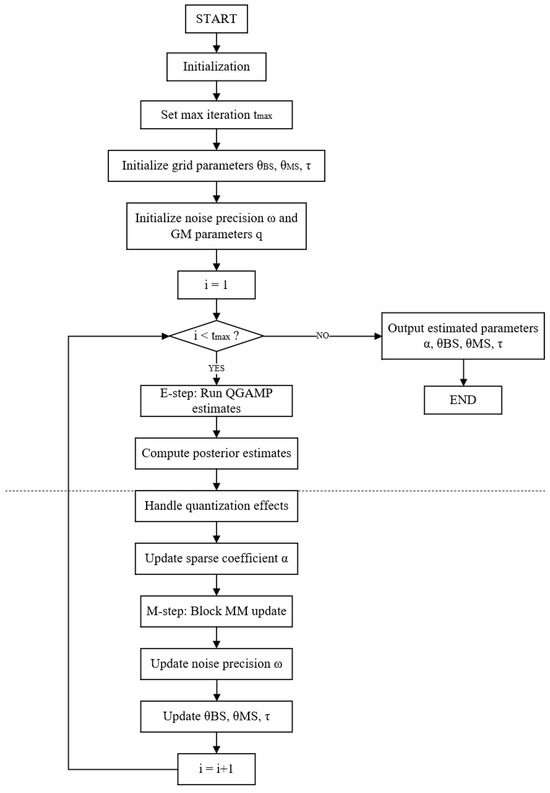
Figure 2.
EM-QGAMP algorithm flowchart.
4.3. Complexity Analysis
In this subsection, we conduct a complexity analysis of the proposed algorithm to different grids and later include a discussion of the complexity of the proposed algorithm with respect to other baseline algorithms mentioned in the simulation section.
In the fixed grid, the computational complexity primarily arises from two aspects: channel matrix construction and sparse channel estimation. Constructing the channel matrix incurs a complexity of , where the total number of grid points is , and G is the length of the received signal. Sparse channel estimation, which employs OMP algorithm, has a complexity of , where L is the number of propagation paths. Thus, the total computational complexity of the fixed grid approach can be expressed as . As an adjustable alternative, our proposed algorithm includes an iterative process to dynamically refine grid points, adding additional computational overhead. Over T iterations, the overall computational complexity of the proposed algorithm is . This analysis highlights the trade-offs between the two methods: the fixed grid approach has lower computational complexity and runtime but suffers from higher quantization errors due to the coarse grid. In contrast, although the adjustable grid approach incurs higher computational costs due to iterative refinement, it can achieve higher estimation accuracy, especially in sparse or dynamic channel environments.
The complexity of channel estimation algorithms mentioned in the simulation is analyzed and compared in Table 1. The complexity of ML algorithms grows exponentially with the number of paths, making them unsuitable for practical large-scale scenarios. The SOMP-SAGE algorithm has lower complexity when the number of channel paths is small, but as the number of antennas and paths increases, computational errors become significantly more pronounced. HT-NARM [29], a novel algorithm is proposed called reweighted atomic norm minimization (NRAM), which combines the Hankel–Toeplitz block model with multiple measurement vectors (MMVs) to solve the channel estimation problem. Although the proposed EM-QGAMP algorithm is more complex, it achieves higher estimation accuracy in challenging environments.

Table 1.
Complexity comparison.
5. Simulation
In this section, we provide the simulation results to show the superiority of the proposed algorithm. We consider that the BS has an ULA with antennas serving a single user, and the numbers receiving antennas are set to , where the number of channel paths between the BS and user is set to . The UL AoAs and DL AoDs are assumed to be identical according to angle reciprocity. All the AoA/AoDs are randomly generated and then kept the same in all Monte-Carlo tests. The channel complex gain is independent and identically distributed as (0, 1) for all paths. The hardware limitations of low-resolution ADCs are given by (11). We set the UL/DL carrier frequency as = 60 GHz, = 62 GHz, B = 100 MHz and . The number of sequentially transmitted signals is and the grid parameters are set as , and . Each element of pilot sequence along sequentially transmitted symbols indexed by g and different subcarriers indexed by n, is obtained as a zero mean complex Gaussian random variable, then normalized , . Moreover, we compare the performance of the proposed algorithm with the following baselines: the ML algorithm, the SOMP-SAGE algorithm, and the proposed EM-QGAMP algorithm for only UL channel estimation. Figure 3, Figure 4, Figure 5 and Figure 6 are all completed under 3-bit quantization.
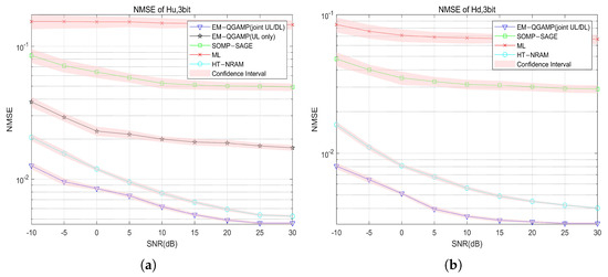
Figure 3.
NMSE of UL/DL channel vs. SNR, (a) NMSE of UL channel; (b) NMSE of DL channel.
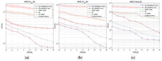
Figure 4.
NMSE of channel parameters vs. SNR, (a) NMSE of ; (b) NMSE of ; and (c) NMSE of delay.
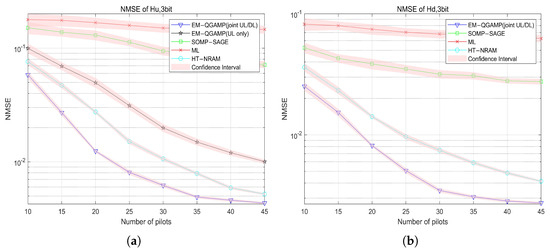
Figure 5.
NMSE of UL/DL channel vs. pilot numbers: (a) NMSE of UL channel; (b) NMSE of DL channel.
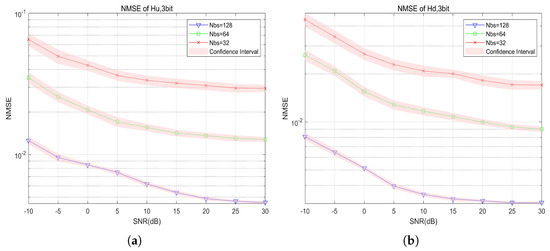
Figure 6.
NMSE of UL/DL channel vs. SNR with different antenna numbers: (a) NMSE of UL channel; and (b) NMSE of DL channel.
Figure 3 shows the curve of the NMSE of the UL and DL channel estimation as the SNR changes. It can be seen from the results that the ML algorithm performs the worst. On the contrary, the algorithm proposed in this paper achieves the best estimation effect. Specifically, at dB, the NMSE performance of the proposed algorithm in the UL channel is nearly higher than that of the traditional ML algorithm and higher than that of the advanced HT-NARM algorithm. This is due to the use of the QGAMP algorithm to handle the quantization process. Compared with algorithms that only target UL channel estimation, the algorithm proposed in this paper has the advantage of using joint UL and DL channel estimation. Experimental results show that this joint estimation method is better than the method that only estimates the DL channel.
Figure 4 shows the curve of the NMSE of the estimated angles of the base station, the angles of user terminal and delay as the SNR changes. Compared with the results shown in Figure 3, the accuracy of the parameter estimation by this algorithm is significantly better than that of UL and DL channel estimation. For all quantization bits, the proposed algorithm is better than the other four baseline algorithms in parameter estimation, and can achieve good results even under low-resolution quantization conditions.
Figure 5 shows the curve of the UL and DL channels as the number of pilot symbols changes. As the number of pilot symbols continues to increase, the NMSE of various channel estimation algorithms gradually decreases. At any fixed number of pilot symbols, our proposed algorithm outperforms the baseline algorithm. More importantly, even if the number of pilot symbols is much smaller than the number of antennas, our algorithm can still perform very well, which fully proves that the compressed sensing technology has obvious advantages in channel estimation for Massive MIMO systems.
Figure 6 shows the curves of the UL and DL channels as the number of antenna at the base station changes with three-bit quantization, from which it can be seen that the estimated NMSE of both the UL and DL channels decreases as the number of antenna increases. This figure highlights the importance of antenna configuration in improving signal quality in communication systems, and also reflects its key role in reducing communication system errors.
Figure 7 shows the curve of the UL and DL channels as the SNR changes with one-bit to three-bit quantization, where it can be seen that the NMSE of the estimated UL and DL channels decreases as the quantization bit number increases. Compared to the DL channel, the accuracy of UL channel estimation improves significantly as the number of quantization bits increases, because the received UL signal is directly affected by the low-resolution ADC.
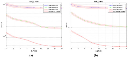
Figure 7.
NMSE of UL/DL channel vs. SNR under 1 to 3 bit: (a) NMSE of UL channel; and (b) NMSE of DL channel.
Figure 8 shows the curve of the CPU time as the number of pilot symbols changes. It can be seen that no matter which algorithm is used, the CPU time will increase linearly with the increase in the number of pilot symbols. The proposed algorithm performs better with the same number of pilot symbols, but it inevitably takes more processing time. Therefore, in practical applications, a trade-off between complexity and performance needs to be considered.
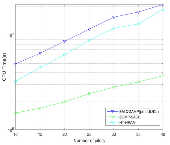
Figure 8.
CPU time vs. pilot numbers.
In conclusion, the algorithm proposed in this paper can obviously achieve better performance in channel parameter estimation and UL and DL channel estimation. This enhancement can be attributed to the modeling of an adjustable angle/multipath delay grid, the concurrent estimation of the UL and DL channels, and the sophisticated handling of the quantization process within the algorithm, which collectively confer upon it a performance advantage over the baseline algorithm. This algorithm can be applied in most situations. However, in environments with extremely limited computing resources, high complexity may become a prominent problem. In addition, the simulation is based on a flat fading channel model and assumes that the UE is equipped with perfect ADCs/DACs. However, in actual systems, more complex channel models and various hardware impairment-related situations need to be considered.
6. Conclusions
In this paper, the joint UL and DL channel estimation problems for mmWave massive MIMO with low-resolution ADCs have been studied. We adopt a strategy that combines quantized UL and DL signals at the BS for joint estimation. The received signal is then reconstructed into a sparse model, and then parameter estimation is performed using the EM-QGAMP algorithm. This method can make full use of the advantages of joint UL/DL estimation to make up for the UL channel estimation problem under low quantization conditions. In addition, we use parameterized estimation method, which greatly reduces the cost of channel estimation.
Author Contributions
Conceptualization, S.W. and Y.W.; methodology, S.W.; formal analysis, S.W.; software, C.H.; visualization, C.H.; resources, Y.W.; data curation, C.H.; writing—original draft preparation, S.W. and C.H.; writing—review and editing, Y.W.; supervision, Y.W.; funding acquisition, Y.W. All authors have read and agreed to the published version of the manuscript.
Funding
This work was supported in part by the Science and Technology Research and Development Program of China State Railway Group Co., Ltd. (No. L2023G004).
Data Availability Statement
The data presented in this study are available on request from the corresponding author.
Conflicts of Interest
Author Songxu Wang was employed by Equipment Technology Center of National Railway Administration of China. The remaining authors declare that the research was conducted in the absence of any commercial or financial relationships that could be construed as a potential conflict of interest.
Correction Statement
This article has been republished with a minor correction to the Funding statement. This change does not affect the scientific content of the article.
Appendix A. Proof of Properties of the Surrogate Function in (46)
Appendix A.1
Following Jensen’s inequality, for any distribution of , we have
where the equality only holds when the estimated parameters are equal to the optimal solution, which makes for some constant c. Such a can be found by
and we have
in this way, the convergence can be proved.
Appendix B. Proof of Function in (47)
Since we assume distributed as Gamma distribution, we have
then, we can simplify the surrogate function as follows, where the items independent of are dropped.
The surrogate function of can be deviated in the same way. Then, we can get a unique optimal point of by taking the derivative of the surrogate function easily.
Appendix C. Proof of the Derivation of θBS Surrogate Function
In the above, we have obtained the log-likelihood function of
First, we consider the derivation of DL related item. If we assume that , we have
where
which follows
where , and can be obtained by
where
where
Finally, we can derive as follows
Then, we consider the derivative of the UL-related item. For , we can obtain it by
which follows
and can be obtained by
which follows
where . Finally, we can derive as follows
References
- Sun, H.; Ng, C.; Huo, Y.; Hu, R.Q.; Wang, N.; Chen, C.M.; Vasudevan, K.; Yang, J.; Montlouis, W.; Ayanda, D.; et al. Massive MIMO. In Proceedings of the 2023 IEEE Future Networks World Forum (FNWF), Baltimore, MD, USA, 13–15 November 2023; pp. 1–70. [Google Scholar]
- Dreifuerst, R.M.; Heath, R.W. Massive MIMO in 5G: How Beamforming, Codebooks, and Feedback Enable Larger Arrays. IEEE Commun. Mag. 2023, 61, 18–23. [Google Scholar] [CrossRef]
- Walden, R.H. Analog-to-digital converter survey and analysis. IEEE J. Sel. Areas Commun. 1999, 17, 539–550. [Google Scholar] [CrossRef]
- Murmann, B. Energy limits in A/D converters. In Proceedings of the 2013 IEEE Faible Tension Faible Consommation, Paris, France, 20–21 June 2013; pp. 1–4. [Google Scholar]
- Wang, F.; Fang, J.; Li, H.; Chen, Z.; Li, S. One-bit quantization design and channel estimation for massive MIMO systems. IEEE Trans. Veh. Technol. 2018, 67, 10921–10934. [Google Scholar] [CrossRef]
- Liu, F.; Zhu, H.; Li, C.; Li, J.; Wang, P.; Orlik, P.V. Angular-domain channel estimation for one-bit massive MIMO systems: Performance bounds and algorithms. IEEE Trans. Veh. Technol. 2020, 69, 2928–2942. [Google Scholar] [CrossRef]
- Risi, C.; Persson, D.; Larsson, E.G. Massive MIMO with 1-bit ADC. arXiv 2014, arXiv:1404.7736. [Google Scholar]
- Xu, L.; Qian, C.; Gao, F.; Zhang, W.; Ma, S. Angular domain channel estimation for mmWave massive MIMO with one-bit ADCs/DACs. IEEE Trans. Wirel. Commun. 2020, 20, 969–982. [Google Scholar] [CrossRef]
- Rashid, M.; Naraghi-Pour, M. Clustered Sparse Channel Estimation for Massive MIMO Systems by Expectation Maximization-Propagation (EM-EP). IEEE Trans. Veh. Technol. 2023, 72, 9145–9159. [Google Scholar] [CrossRef]
- Choi, J.; Mo, J.; Heath, R.W. Near maximum-likelihood detector and channel estimator for uplink multiuser massive MIMO systems with one-bit ADCs. IEEE Trans. Commun. 2016, 64, 2005–2018. [Google Scholar] [CrossRef]
- Liu, F.; Zhu, H.; Li, J.; Wang, P.; Orlik, P.V. Massive MIMO channel estimation using signed measurements with antenna-varying thresholds. In Proceedings of the 2018 IEEE Statistical Signal Processing Workshop (SSP), Freiburg im Breisgau, Germany, 10–13 June 2018; IEEE: Piscataway, NJ, USA, 2018; pp. 188–192. [Google Scholar]
- Wen, C.K.; Wang, C.J.; Jin, S.; Wong, K.K.; Ting, P. Bayes-optimal joint channel-and-data estimation for massive MIMO with low-precision ADCs. IEEE Trans. Signal Process. 2015, 64, 2541–2556. [Google Scholar] [CrossRef]
- Shahmansoori, A.; Garcia, G.E.; Destino, G.; Seco-Granados, G.; Wymeersch, H. Position and orientation estimation through millimeter-wave MIMO in 5G systems. IEEE Trans. Wirel. Commun. 2017, 17, 1822–1835. [Google Scholar] [CrossRef]
- Habibur Rahman, M.; Abrar Shakil Sejan, M.; Abdul Aziz, M.; Tabassum, R.; Baik, J.I.; Song, H.K. Deep Learning Based One Bit-ADCs Efficient Channel Estimation Using Fewer Pilots Overhead for Massive MIMO System. IEEE Access 2024, 12, 64823–64836. [Google Scholar] [CrossRef]
- Zhang, R.; Tan, W.; Li, S.; Tang, M. Channel Estimation for IRS-Assisted mmWave Massive MIMO Systems in Mixed-ADC Architecture. IEEE Internet Things J. 2024, 11, 9969–9978. [Google Scholar] [CrossRef]
- Liu, A.; Zhu, F.; Lau, V.K. Closed-loop autonomous pilot and compressive CSIT feedback resource adaptation in multi-user FDD massive MIMO systems. IEEE Trans. Signal Process. 2016, 65, 173–183. [Google Scholar] [CrossRef]
- Xie, H.; Gao, F.; Jin, S.; Fang, J.; Liang, Y.C. Channel Estimation for TDD/FDD Massive MIMO Systems with Channel Covariance Computing. IEEE Trans. Wirel. Commun. 2018, 17, 4206–4218. [Google Scholar] [CrossRef]
- Huang, Y.D.; Liang, Y.C.; Gao, F. Channel Estimation in FDD Massive MIMO Systems Based on Block-Structured Dictionary Learning. In Proceedings of the 2019 IEEE Global Communications Conference (GLOBECOM), Waikoloa, HI, USA, 9–13 December 2019; pp. 1–6. [Google Scholar]
- Zhao, Y.; Teng, Y.; Liu, A.; Wang, X.; Lau, V.K.N. Joint UL/DL Dictionary Learning and Channel Estimation via Two-Timescale Optimization in Massive MIMO Systems. IEEE Trans. Wirel. Commun. 2024, 23, 2369–2382. [Google Scholar] [CrossRef]
- Jee, J.; Park, H. Deep Learning-Based Joint Optimization of Closed-Loop FDD mmWave Massive MIMO: Pilot Adaptation, CSI Feedback, and Beamforming. IEEE Trans. Veh. Technol. 2024, 73, 4019–4034. [Google Scholar] [CrossRef]
- Zia, M.U.; Xiang, W.; Vitetta, G.M.; Huang, T. Deep Learning for Parametric Channel Estimation in Massive MIMO Systems. IEEE Trans. Veh. Technol. 2023, 72, 4157–4167. [Google Scholar] [CrossRef]
- Ding, Y.; Rao, B.D. Compressed downlink channel estimation based on dictionary learning in FDD massive MIMO systems. In Proceedings of the 2015 IEEE Global Communications Conference (GLOBECOM), San Diego, CA, USA, 6–10 December 2015; IEEE: Piscataway, NJ, USA, 2015; pp. 1–6. [Google Scholar]
- Ding, Y.; Rao, B.D. Dictionary Learning-Based Sparse Channel Representation and Estimation for FDD Massive MIMO Systems. IEEE Trans. Wirel. Commun. 2018, 17, 5437–5451. [Google Scholar] [CrossRef]
- Zhang, R.; Zhao, H.; Jia, S.; Shan, C. Joint channel estimation algorithm based on structured compressed sensing for FDD multi-user massive MIMO. In Proceedings of the 2016 IEEE 13th International Conference on Signal Processing (ICSP), Chengdu, China, 6–10 November 2016; IEEE: Piscataway, NJ, USA, 2016; pp. 1202–1207. [Google Scholar]
- Wang, Z.; Li, Y.; Wang, C.; Ouyang, D.; Huang, Y. A-OMP: An Adaptive OMP Algorithm for Underwater Acoustic OFDM Channel Estimation. IEEE Wirel. Commun. Lett. 2021, 10, 1761–1765. [Google Scholar] [CrossRef]
- Zhu, F.; Liu, A.; Lau, V.K. Joint channel estimation and data recovery of communication systems with sub-Nyquist receiver. In Proceedings of the 2015 IEEE International Conference on Communications (ICC), London, UK, 8–12 June 2015; IEEE: Piscataway, NJ, USA, 2015; pp. 2614–2619. [Google Scholar]
- Tibshirani, R. Regression shrinkage and selection via the lasso. J. R. Stat. Soc. Ser. B (Methodol.) 1996, 58, 267–288. [Google Scholar] [CrossRef]
- Vila, J.P.; Schniter, P. Expectation-maximization Gaussian-mixture approximate message passing. IEEE Trans. Signal Process. 2013, 61, 4658–4672. [Google Scholar] [CrossRef]
- Zhu, L.; Xiong, Y.; Li, Z.; Guan, Y.; Chu, Z.; Zhu, Z.; Xiao, P.; Wang, C.L. A Novel Gridless Uplink/Downlink Channel Estimation Method for Millimeter Wave MIMO-OFDM Systems. IEEE Trans. Wirel. Commun. 2025, 24, 3780–3793. [Google Scholar] [CrossRef]
Disclaimer/Publisher’s Note: The statements, opinions and data contained in all publications are solely those of the individual author(s) and contributor(s) and not of MDPI and/or the editor(s). MDPI and/or the editor(s) disclaim responsibility for any injury to people or property resulting from any ideas, methods, instructions or products referred to in the content. |
© 2025 by the authors. Licensee MDPI, Basel, Switzerland. This article is an open access article distributed under the terms and conditions of the Creative Commons Attribution (CC BY) license (https://creativecommons.org/licenses/by/4.0/).