Communication Delay Prediction of DPFC Based on SAR-ARIMA-LSTM Model

Abstract

Communication delay, as a key factor restricting the rapid and accurate transmission of data in the smart grid, will affect the collaborative operation of power electronic devices represented by the Distributed Power Flow Controller (DPFC), and further affect the construction and safe and stable operation of the new power system. Aiming at the problem of DPFC communication delay prediction, this paper proposes a new SAR-ARIMA-LSTM hybrid prediction model. This model introduces the spatial autoregressive model (SAR) on the basis of the traditional ARIMA-LSTM model to extract the spatial correlation between devices caused by geographical location and communication load, and then combines ARIMA-LSTM prediction. The experimental structure shows that compared with the traditional ARIMA-LSTM model, the model proposed in this paper predicts that RMSE decreases from 1.59 to 1.2791 and MAE decreases from 1.27 to 1.0811, with a reduction of more than 14%. The method proposed in this paper can effectively reduce the communication delay prediction data of DPFC at different spatial positions, has a stronger ability to handle high-delay fluctuations, and provides a new technical approach for improving the reliability of the power grid communication network.

1. Introduction

The vigorous development of new energy power generation will accelerate the transformation of future power systems towards low-carbonization and intelligence [1]. As an important power electronic device, the distributed power flow controller (DPFC) plays a key role in enhancing the flexibility and reliability of power grid operation. Recent studies have demonstrated that DPFC can significantly improve power flow distribution by enabling distributed installation on transmission lines, which overcomes the limitations of traditional centralized FACTS devices and provides enhanced system loadability [2]. Furthermore, the optimal configuration of DPFC devices has been shown to effectively enhance system capacity while considering economic performance, particularly through mixed integer linear programming approaches that balance loadability improvements with investment costs [3].

In the distributed control system of DPFC, communication delay usually fluctuates over time and is affected by dynamic factors such as network congestion and data load, showing obvious time dependence and trends. Research shows that a communication delay may cause system instability, degradation of control performance, and even equipment damage [4]. The significance of communication delay prediction becomes more pronounced when considering that DPFC devices must coordinate their operations across spatially distributed locations, where network latency can critically affect the real-time control performance required for power flow regulation [2]. This spatial distribution characteristic of DPFC systems introduces additional complexity in delay prediction compared to centralized control systems, as the communication paths between devices may traverse different network segments with varying congestion levels and transmission characteristics.

Therefore, accurately predicting the communication delay between DPFC devices is of great significance for the operation and optimization of power systems.

At present, time series prediction mainly includes two categories: traditional statistical models and deep learning models [5]. Traditional prediction models include the historical average (HA) model, autoregressive (AR) model, autoregressive moving average (ARMA) model, autoregressive integrated moving average (ARIMA) model, etc. [6]. Traditional prediction models are relatively simple and have good theoretical interpretability for time series prediction problems, but they cannot capture the complex nonlinear models hidden in the data. With the development of artificial intelligence technology, more and more studies use deep neural networks to predict communication traffic. Common models include artificial neural networks (ANNs) and its various variants, recurrent neural networks (RNNs), convolutional neural networks (CNNs), and gated recurrent units (GRUs) based on the RNN structure [7]. However, single deep learning models have problems such as slow convergence speed and easy to fall into local optimal solutions [8], making it difficult to capture both linear and nonlinear features of the data simultaneously.

The ARIMA-LSTM hybrid model, by integrating the advantage of the ARIMA model in capturing the linear trend of data and the ability of the LSTM network to extract complex nonlinear features of data [9], compensates for the shortcomings of a single model and can effectively improve the accuracy of time series prediction. The ARIMA-LSTM hybrid model has demonstrated excellent predictive performance in multiple fields [10,11,12], and maintains a high accuracy rate in short-term predictions, which aligns with the high-precision prediction requirements for communication delay in distributed power flow control (DPFC) devices. The effectiveness of such hybrid approaches has been further validated in recent traffic flow prediction studies, where ARIMA-LSTM combinations have shown superior performance in capturing both temporal dependencies and nonlinear spatio-temporal dynamics [5], characteristics that are particularly relevant for communication delay prediction in distributed systems.

However, considering the differences in the roles and priorities of different DPFC devices in the system, as well as the influence of spatial factors such as the distance between devices and the degree of communication congestion in their respective areas on delay, for instance, in densely populated areas, the probability of communication delay significantly increases and the range of delay data is large, and it is difficult to achieve high-precision prediction solely relying on time series models. The spatial dimension becomes increasingly critical when considering that DPFC devices operate in a distributed manner across transmission networks, where the physical topology and network infrastructure characteristics can significantly influence communication patterns [3]. The optimal placement and configuration of DPFC devices not only affects power flow control effectiveness but also determines the communication network topology and associated delay characteristics.

Therefore, this paper proposes a hybrid prediction method combining the spatial autoregressive model (SAR) with the ARIMA-LSTM model.

This method first utilizes the spatial autoregressive model (SAR) to extract the spatial characteristics of DPFC communication delay, considering the spatial distance factor of the importance of device communication. Then, the ARIMA model is adopted to predict the linear trend of the adjusted data, and the residuals are used as the LSTM network to capture nonlinear features. Finally, the linear and nonlinear prediction results are combined to obtain the final predicted value. The main contributions of this study include the following: (1) a communication delay prediction method considering the spatial characteristics of DPFC was proposed, combining the SAR model with the ARIMA-LSTM hybrid model, which improved the prediction accuracy; (2) in practical applications, this method can be used for the dynamic adjustment of resource allocation and control strategy optimization of distributed devices in power systems, thereby reducing the risk of communication failures.

2. Materials and Methods

2.1. SAR Model

2.1.1. Model Construction

Traditional communication delay prediction methods usually only consider the communication delays of the base station and the device itself, while ignoring the spatial characteristics of the area where the device is located. With the continuous development of the power grid, the grid structure has become increasingly complex, resulting in significant differences in the regional characteristics of different power flow controllers. Therefore, for the delay prediction of different devices, their spatial characteristics should be considered even more [13]. 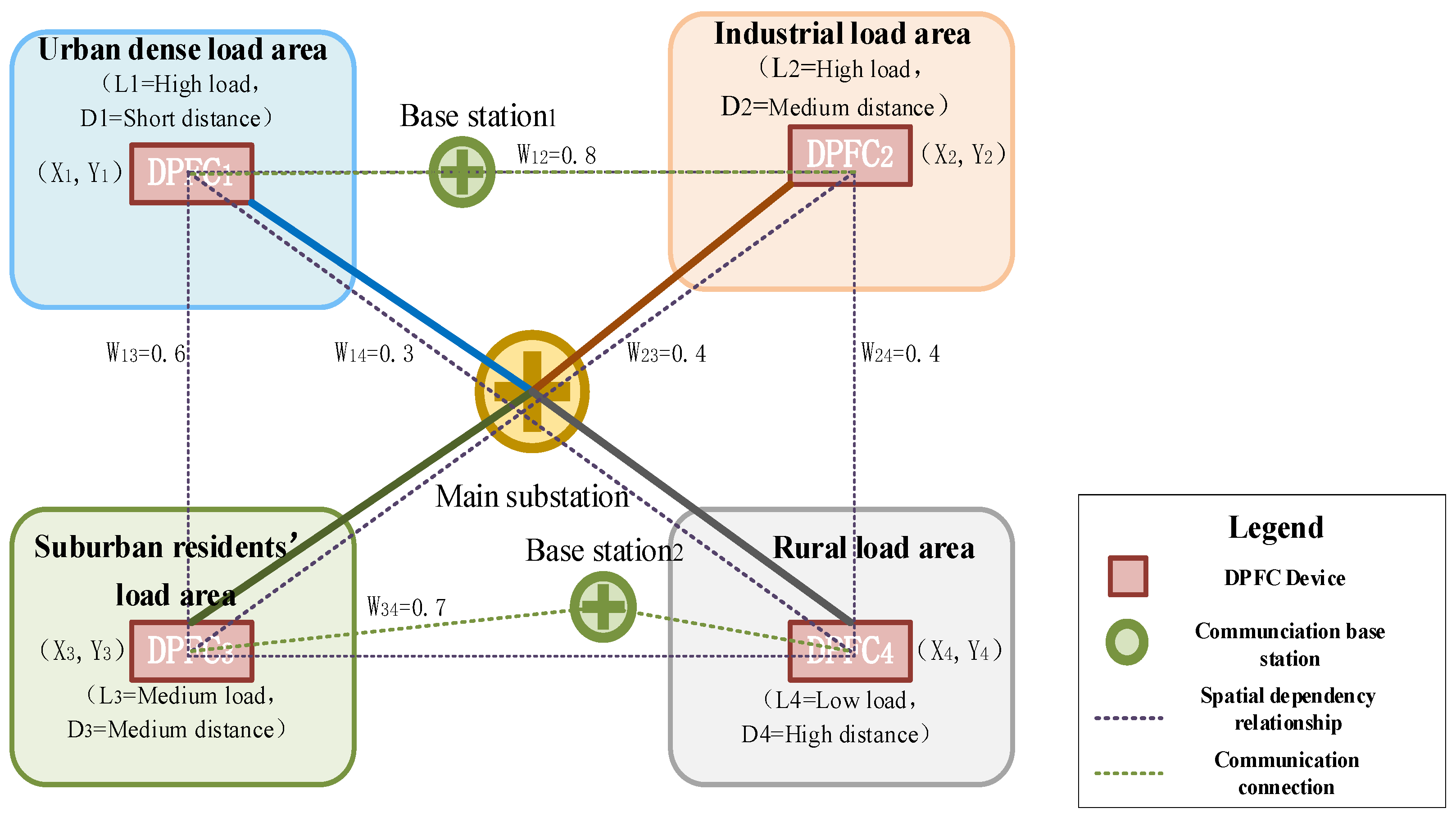Figure 1 shows a spatial schematic diagram of a power system with distributed devices, in which each spatial area is equipped with a DPFC device.

This figure indicates that there are differences in the types of areas where different devices are located in the distribution network, and the influencing factors of spatial characteristics among different devices are also different.

The core idea of the spatial autoregressive model (SAR), as a regression model considering spatial correlation, is to capture the dependency characteristics of spatial data through the spatial weight matrix W, thereby overcoming the deviation caused by the traditional regression model ignoring spatial correlation [14]. The SAR model can be expressed as follows:

$$y=\rho Wy+X\beta +\epsilon$$

(1)

Among them, $\rho$ is the spatial autoregressive coefficient, quantifying the degree of spatial dependence; W is the spatial weight matrix; X is the matrix of independent variables; $\beta$ is the regression coefficient vector; and $\epsilon$ is the error vector that follows a normal distribution. The spatial dependency $\rho Wy$ represents the spatial dependency among the dependent variables. The weight matrix W defines the spatial relationship between regions, and the coefficient measures the strength of the spatial dependency. The coefficient $\rho$ measures the strength of spatial dependence, and the explanatory variable term $X\beta$ represents the direct influence of the explanatory variable on the dependent variable.

In order to better reflect the spatial dependence among various power flow controllers, this paper first constructs a spatial weight matrix W applicable to DPFC devices. Suppose there is a power flow controller in the system. The position coordinate of each controller is $n$, and the corresponding power flow capacity of the line is $(x_i,y_i)$. The spatial weight matrix W is a symmetric matrix of $(n\times n)$, where element $w_{ij}$ represents the spatial weight between the i-th and j-th controllers.

Common construction methods include distance-based threshold matrices, proximity matrices (Queen or Rook proximity), etc. Considering that the communication delay of DPFC devices in the power system is related to the spatial distance, this paper uses the weight definition method based on the distance threshold. This method can reflect the actual spatial dependency relationship between DPFC nodes more accurately. By flexibly setting the distance threshold, it can effectively control the connection density between DPFC devices and improve the scalability of the model. The method is defined as follows:

$$w_{ij}=\left\{\begin{array}{cc}{\displaystyle \frac{1}{d_{ij}}}& \mathrm{if}{d}_{ij}<\theta \\ 0& \mathrm{otherwise}\end{array}\right.$$

(2)

Among them, $d_{ij}$ is the Euclidean distance between the i-th and j-th controllers, and $\theta$ is the set distance threshold. Suppose there are $n$ controllers in the system, and the position coordinate of each controller is $(x_{1i},x_{2i})$, corresponding to a power flow capacity of $c_i$. The communication delay vector y can be expressed as follows: ${\mathrm{y}=[\mathrm{y}}_1{,\mathrm{y}}_2,\dots {,\mathrm{y}}_n{]}^T$. Construct the explanatory variable matrix X containing the constant term, position coordinates, and power flow capacity:

$$X=\left[\begin{array}{cccc}1& x_{11}& x_{21}& C_1\\ 1& x_{12}& x_{22}& C_2\\ ⋮& ⋮& ⋮& ⋮\\ 1& x_{1n}& x_{2n}& C_n\end{array}\right]$$

(3)

When constructing a multivariate spatial autoregressive model, we add position coordinates and power flow capacity as additional explanatory variables to the model. The specific model form is as follows:

$$y_t=p_t\ast W_t\ast y_t+U_t{+\mathrm{a}}_t\ast I+{\mathrm{b}}_t\ast L+c_t\ast D+{\epsilon }_t$$

(4)

Among them, $U_t$ represents the global intercept, indicating the average level of the overall communication delay; I indicates the importance of the device; L indicates the load size of the power supply area where the device is located, and D indicates the distance between the base station and the power supply area.

2.1.2. Model Parameter Estimation

The parameter estimation of the SAR model is a key step in model construction. This paper adopts the maximum likelihood estimation method. This method fully considers the influence of the spatially dependent structure on the error distribution and has significant advantages when dealing with spatial autocorrelation. By introducing the Jacobian determinant to correct the probability density transformation caused by the spatial structure, the Jacobian determinant is as follows:

$$\left|A\right|=|I-\rho W|$$

(5)

Maximizing the likelihood function L is equivalent to minimizing the sum of squared deviations corrected by Jacob. The spatial term in Jacob’s determinant $\left|A\right|$ makes it different from the ordinary least squares estimation. Therefore, it is necessary to ensure that $\left|A\right|$ > 0, that is, $|I-\rho W|$ > 0. Furthermore, for maximum likelihood estimation, it is necessary to solve the first-order partial derivative of the parameter to be estimated and set it equal to 0 to obtain the parameter estimate value:

$$d=(\partial L/\partial \theta )=0$$

(6)

The component of d is as follows:

$$\partial L/\partial \beta ={ϵ}^{\prime }X$$

(7)

$$\partial L/\partial \rho =-\mathrm{tr}(A^{-1}W)+{ϵ}^{\prime }Wy$$

(8)

By using numerical methods to solve the above nonlinear equation system, the maximum likelihood estimation of the parameters $\rho$ and $\beta$ can be obtained.

2.1.3. Model Evaluation

After the construction of the multivariate spatial autoregressive model is completed, it is crucial to evaluate its fitting effect. The evaluation results can not only reflect the model’s ability to interpret data but also provide a basis for subsequent optimization. This paper conducts a comprehensive assessment using indicators such as pseudo $R^2$. In addition, there is the maximum likelihood pair value (Log-Likelihood, LIK), Akaike information criterion (AIC), and Schwarz Criterion (SC) [15].

Firstly, pseudo $R^2$ is an important indicator for measuring the goodness of fit of a model, which is especially applicable to nonlinear models and spatial regression models. Its calculation formula is as follows:

$$R^2=1-{\displaystyle \frac{{\displaystyle \sum _{i=1}^n}{(y_i-{\widehat{y}}_i)}^2}{{\displaystyle \sum _{i=1}^n}{(y_i-\overline{y})}^2}}$$

(9)

Among them, ${\mathrm{y}}_i$ represents the predicted value of the model, and y is the mean of the observed values. The value range of pseudo $R^2$ is between 0 and 1. The closer it is to 1, the better the model fitting effect. However, it should be noted that pseudo $R^2$ is not an absolute standard but a relative reference value, mainly used to compare the fitting effects among different models. By calculating pseudo $R^2$, we can initially determine whether the model can effectively capture the spatial dependence and trend characteristics in the data.

Secondly, the maximum likelihood pairwise value (LIK) is another important indicator for measuring the goodness of fit of the model. It is calculated based on the logarithmic likelihood function, and the specific formula has been given in the previous text. The higher the LIK value is, the better the model fitting effect is. The LIK value can be directly used to compare the fitting effects among different models. The larger the value, the better the model. Through the calculation and analysis of the LIK value, the fitting effect of the model can be further verified, and it can be ensured that the selected model has high explanatory power and prediction accuracy.

Furthermore, the Chichi Information Criterion (AIC) and the Schwartz Information Criterion (SC) are two commonly used model selection criteria. They not only consider the fitting effect of the model but also the complexity of the model. The calculation formulas of AIC and SC are, respectively, as follows:

$$AIC=2k-2\log (L)$$

(10)

$$SC=k\log (n)-2\log (L)$$

(11)

Among them, k is the number of parameters in the model, L is the maximum likelihood estimate, and n is the sample size. The smaller the AIC and SC values are, the better the model is. These two criteria can strike a balance between the fitting effect and the model complexity, avoiding the problem of overfitting. By comparing the AIC and SC values of different models, the optimal model can be determined, thereby improving the generalization ability and practical application value of the model.

2.2. ARIMA Model

The Differential Integrated Moving Average Autoregressive model (ARIMA) is a statistical model widely used in time series prediction. It combines three parts: autoregressive (AR), differential (I), and moving average (MA), and can effectively capture characteristics such as trends, seasonality, and noise in time series [15]. The general expression of the ARIMA (p, d, q) model is as follows:

$$Y_{\mathrm{t}}=c+{\varphi }_1{Y}_{t-1}+{\varphi }_2{Y}_{t-2}+\dots +{\varphi }_p{Y}_{t-p}+{\theta }_1{\epsilon }_{t-1}+{\theta }_2{\epsilon }_{t-2}+\dots +{\theta }_q{\epsilon }_{t-q}+{\epsilon }_t$$

(12)

Among them, $Y_{\mathrm{t}}$ is the time series value at the current time t, and ${\varphi }_i(i=1,2\dots p)$ and ${\theta }_j(j=1,2\dots q)$ are the auto-regressive term coefficients and the moving average term coefficients, respectively. The relevant principles of the ARIMA model are as follows:

When the communication delay time series $\left\{Y_t\right\}$ conforms to the conditions of a stationary stochastic process, it can be described by the auto-regressive moving average (ARMA) model, as follows:

$$Y_t={\alpha }_1{Y}_{t-1}+{\alpha }_2{Y}_{t-2}+\dots +{\alpha }_p{Y}_{t-p}+e_t-{\beta }_1{e}_{t-1}-{\beta }_2{e}_{t-2}-\dots -{\beta }_q{e}_{t-q}$$

(13)

The model is called the ARMA (p, q) model, where et represents an independent and identically distributed sequence of zero-mean and identically variable white noise. The ARMA (p, q) model combines the auto-regressive (AR) and moving average (MA) parts and has the following characteristic polynomial structure:

The AR auto-regressive characteristic polynomial is as follows:

$$\alpha (x)=1-{\alpha }_{1}x-{\alpha }_2{x}^2-\dots -{\alpha }_p{x}^p$$

(14)

The characteristic equation of AR is as follows:

$$1-{\alpha }_{1}x-{\alpha }_2{x}^2-\dots -{\alpha }_p{x}^p=0$$

(15)

The MA Moving Average Characteristic polynomial is as follows:

$$\beta (x)=1-{\beta }_{1}x-{\beta }_2{x}^2-\dots -{\beta }_q{x}^q$$

(16)

The MA characteristic equation is as follows:

$$1-{\beta }_{1}x-{\beta }_2{x}^2-\dots -{\beta }_q{x}^q=0$$

(17)

When analyzing the communication delay time series of the DPFC device, the original data often present non-stationary characteristics. Therefore, the original data need to be subjected to d order difference processing until a stationary sequence is obtained. If the d order difference $W_t={𝛻}^d{Y}_t$ of a communication delay time series $\left\{Y_t\right\}$ is a stationary ARMA process, it is called the ARIMA differential integration moving average auto-regressive model. If $W_t$ follows ARMA (p, q), then the time series $\left\{Y_t\right\}$ is called the ARIMA (p, d, q) model [16].

The modeling of the ARIMA model mainly consists of three parts: (1) sequence stationarity test and stabilization processing; (2) determination of model structure; (3) parameter estimation and model significance test [17]. This study conducts ARIMA modeling of the DPFC communication delay time series based on the Python3.0 language. The ARIMA model requires that time series data satisfy the stationarity condition, that is, the statistical characteristics of the series (such as the mean, variance, and autocorrelation structure) do not change over time. Because the data are smooth, it does not contain trends and seasonal factors [18]. In this study, ADF was adopted to evaluate the stationarity of communication delay time series. The ADF test is often used to determine whether the time series is stationary [19]. When dealing with non-stationary data, one or two differentiations are used to achieve stationarity, and generally more than two differentiations are not performed. After meeting the stationarity condition and determining the difference order d, the AIC and BIC (SC) criteria were used to evaluate different parameter combinations. By choosing the ARIMA model that minimizes the information criterion, the optimal autoregressive order p and the moving average order q were determined [20]. The smaller the AIC/BIC is, the better. Select the (p, d, q) combination that minimizes AIC or BIC as the final model parameters.

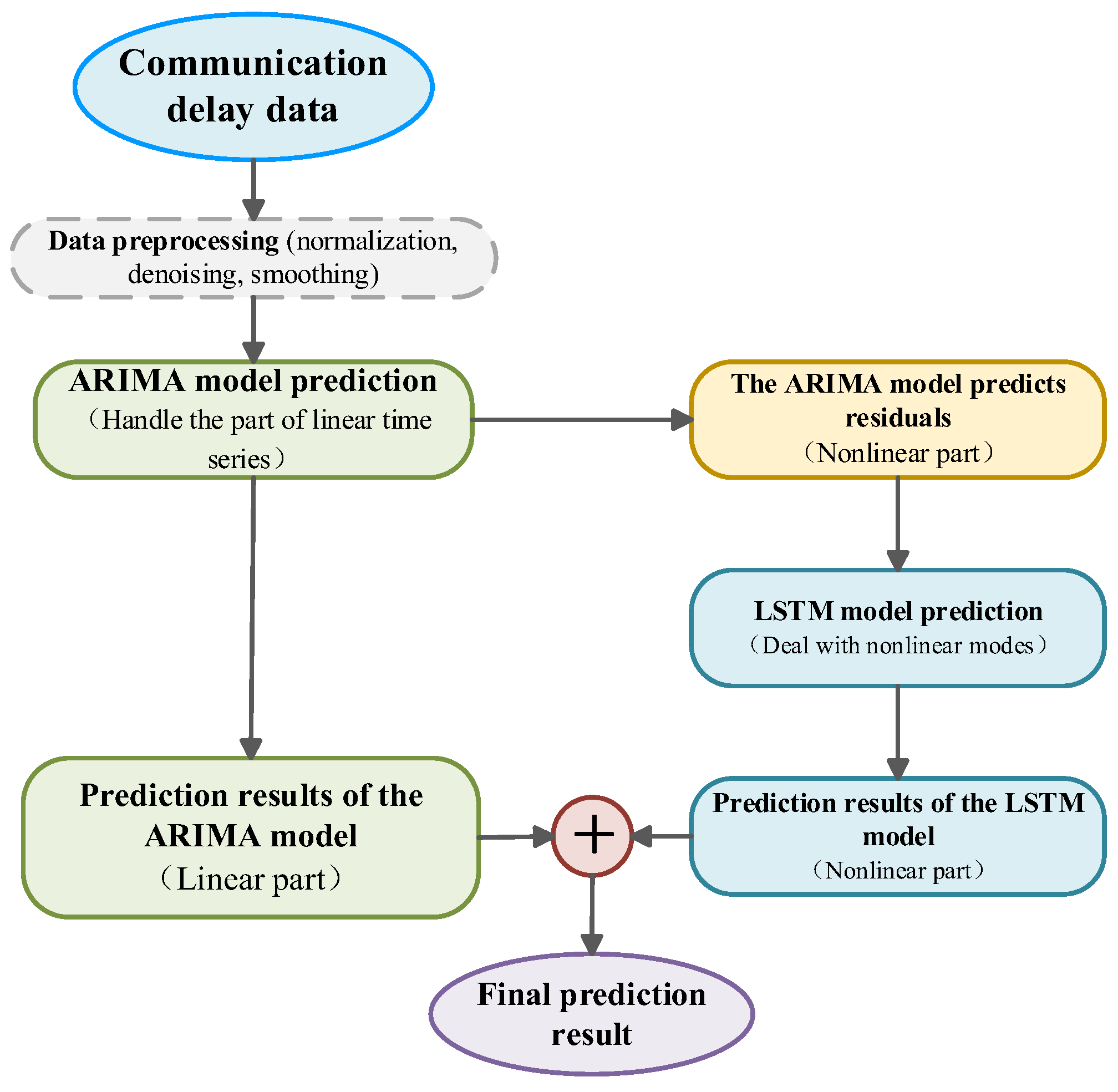
Here, we use the residuals calculated by the ARIMA model as the input of the LSTM model. Since the ARIMA model has identified the linear trend, it is assumed that the residuals contain nonlinear features.

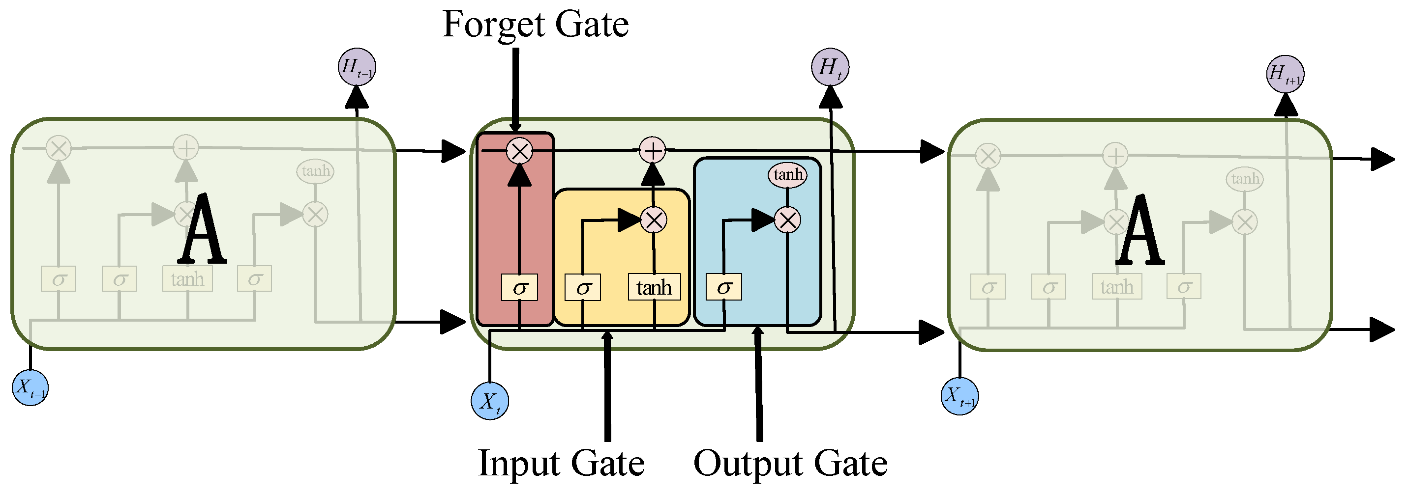
2.3. LSTM Model

Long Short-Term Memory (LSTM) is a special type of recurrent neural network (RNN). The three logical control units in LSTM, namely the input gate, the output gate, and the forgetting gate [21], constitute the basic mechanism of LSTM, and are responsible for the dynamic regulation and control of information storage, update, and output. Each gating unit is connected to a multiplication operation unit. By adjusting the connection weights in the neural network, the input and output of the information flow and the control of the cell state are achieved [22]. The structure of LSTM is shown in Figure 2. The flow diagram of the hybrid model of ARIMA-LSTM is shown in Figure 3.

The forgetting gate: It decides which information should be retained or discarded. It calculates a value between 0 and 1 through a sigmoid function using the current input value $X_t$ and the hidden state $H_{t-1}$ of the previous step [23]. The formula of the forgetting gate is as follows:

$$f_t=\sigma (W_f·[H_{t-1},X_t]+b_f)$$

(18)

Among them, $\sigma$ is the sigmoid function, and $W_f$, respectively, represent the weight matrix and $b_f$ represents the bias of the forget gate. This function generates values close to 0, indicating the information that needs to be forgotten, while values close to 1 indicate the information that needs to be retained.

Input gate: The gate controls whether the input information at the current moment can be updated to the cell state. It calculates a value through the sigmoid function, with a range of (0, 1), to control the degree of influence of the current input. The formula of the input gate is as follows:

$$i_t=\sigma (W_i·[H_{t-1},X_t]+b_i)$$

(19)

The candidate value vector is generated through the tanh activation function, representing a new information candidate that contains the information to be updated to the cell state. The candidate value vector formula and the cell renewal formula are as follows:

$$N_t=\tanh (W_n·[H_{t-1},X_t]+b_n)$$

(20)

$$C_t=C_{t-1}{f}_t+N_t{i}_t$$

(21)

Among them, $C_t$ and $C_{t-1}$ are the cell states at time t and t − 1, respectively, while $W_n$ and $b_n$ represent the weight matrix and bias of the cell states, respectively.

Output gate: The information that determines the state of the cell to the final output. It generates the final output through the weighted processing of the current cell state. The final hidden state of LSTM is the processing result of the cell state controlled by the output gate [24].

$$O_t=\sigma (W_o·[H_{t-1},X_t]+b_o)$$

(22)

$$h_t=O_t\tanh (C_t)$$

(23)

Among them, $W_o$ and $b_o$, respectively, represent the weight matrix and bias of the output gate, and $\tanh (C_t)$ represents the nonlinear transformation of the current cell state.

2.4. ARIMA-LSTM Hybrid Model

At present, there are mainly two methods for time series prediction using the ARIMA-LSTM hybrid model. One of them mainly considers that the ARIMA model, as a traditional prediction model, can fit the linear part in the time series. The LSTM model has the ability of long short-term memory and can effectively fit the nonlinear components in the sequence. Therefore, the residuals of the ARIMA model are taken as the input of LSTM [25]. The cascaded combination of these two models can significantly improve the prediction accuracy and reduce the prediction error. Its specific principle is as follows:

Suppose the communication delay time series is the following:

$$Y_t=L_t+N_t$$

(24)

Among them, $L_t$ is the linear component in the time series, and $N_t$ is the nonlinear component in the time series. By separately analyzing the linear and nonlinear parts in the practical sequence, the limitations of a single model in predicting complex time series are overcome.

The raw communication delay data are first processed by the SAR model to extract spatial correlations. The spatially adjusted communication delay series can be expressed as follows:

$$Y_{spatial,t}=Y_{original,t}-\rho \sum _{j=1}^n{w}_{ij}{Y}_{original,j,t}$$

(25)

where $Y_{spatial,t}$ represents the communication delay data after spatial adjustment, removing the spatial correlation effects identified by the SAR model. This spatial pre-processing ensures that the subsequent ARIMA-LSTM modeling focuses on the temporal patterns rather than being influenced by spatial dependencies.

Spatial-Temporal Decomposition: The spatially-adjusted series is then decomposed according to the hybrid model principle, as follows:

$$Y_{spatial,t}=L_{spatial,t}+N_{spatial,t}$$

(26)

where $L_{spatial,t}$ represents the linear component after spatial adjustment, and $N_{spatial,t}$ represents the nonlinear residual component that contains both temporal nonlinearities and any remaining spatial effects not captured by the SAR model.

Integration Mechanism: The integration of spatial features follows a three-stage sequential process, as follows:

Stage 1—Spatial Feature Extraction: The SAR model extracts spatial correlation coefficients $\rho$ and spatial weights $w_{ij}$ from the raw data, quantifying the spatial dependencies between DPFC devices.

Stage 2—Spatial Adjustment: The original time series is adjusted using the spatial features: ${\epsilon }_{spatial,t}=Y_{original,t}-\rho {\displaystyle \sum _{j=1}^n}{w}_{ij}{Y}_{original,j,t}$. This adjustment removes the spatial correlation component, allowing the ARIMA-LSTM model to focus on temporal patterns.

Stage 3—Hybrid Temporal Modeling: The spatially-adjusted data are then processed by the ARIMA-LSTM hybrid model:

The ARIMA model processes the spatially adjusted data to capture linear temporal trends. The LSTM model processes the spatially adjusted residuals to capture nonlinear temporal patterns.

The modeling process of its hybrid model is shown in Figure 3.

Method Two adopts the optimized weighted combination strategy to integrate the prediction results of the ARIMA model and the LSTM neural network. This method determines the optimal weight coefficients based on the criterion of minimizing the sum of squared errors, and calculates the weighting coefficients of each single model in the form of linear equations. Thus, the ARIMA model and the LSTM neural network model are combined to simulate and predict the changes in communication delay. In the third part of this paper, the solution methods of the two mixed models are compared, and Method One is selected based on the experimental results.

3. Results

3.1. Experimental Scenarios and Data Types

3.1.1. Description of the Experimental Scene

This study takes the distribution network of a provincial power grid in Central China as the experimental scenario. The power grid in this region covers an area of approximately 56,000 square kilometers, including 12 prefecture-level cities and 86 county-level administrative regions, and has typical characteristics of mixed urban–rural power supply. The experiment selected DPFC devices with five key nodes as the research objects, and their spatial distribution is shown in Figure 1. Among them are the following:

DPFC1: Located in the core business district of the provincial capital city, it is surrounded by high-density smart meters and distributed power sources. The peak communication load reaches 280 Mbps and it belongs to a high-priority control node.

DPFC2: Deployed in industrial parks, it is mainly responsible for the power flow control of industrial loads. Affected by the production cycle, communication delays show obvious weekday/weekend periodicity.

DPFC3-DPFC5: They are distributed in rural distribution network areas. Among them, DPFC3 is close to new energy substations (with a photovoltaic installed capacity of 50 MW), while DPFC4/DPFC5 are located in remote mountainous areas where communication infrastructure is relatively weak and vulnerable to weather factors.

3.1.2. Data Composition and Sources

The experimental dataset contains real-time monitoring data from 1 June 2024 to 30 April 2025, with a time resolution of 5 min, and contains a total of 29,200 records (5840 records per DPFC device). The data are sourced from the SCADA system and communication network management platform of the power grid dispatching and control center. The specific variables are shown in

Table 1. Experimental data explanation.

Specific Indicators	Unit	Data Characteristics
Communication delay (Y)	ms	Round-trip delay between devices (0.5–35 ms)
Device longitude and latitude (Long, Lat)		Construct the weight matrix
Line Load capacity (Load)	kW	Real-time active power load of the feeder (peak 1200 kW)
Device importance level (I)	Dimensionless	Power supply reliability grade (1–5 levels)
Sampling Time (Time)	-	Year/month/day/hour
Weather conditions (Weather)	Category variable	Sunny days/cloudy days/rainy days /snowy days

as follows:

3.1.3. Data Partitioning Strategy

Training set: June 2024–February 2025 (a total of 24,160 entries), used for model parameter training and spatial weight matrix optimization.

Validation set: March 2025 (a total of 4464 items), used to adjust the model hyperparameters (such as the spatial autoregressive coefficient ρ of the SAR model and the number of layers of the LSTM network).

Test set: April 2025 (a total of 4576 items), used to independently evaluate the generalization performance of the model and ensure that there is no data leakage in the results.

3.2. The Solution Result of the SAR Model

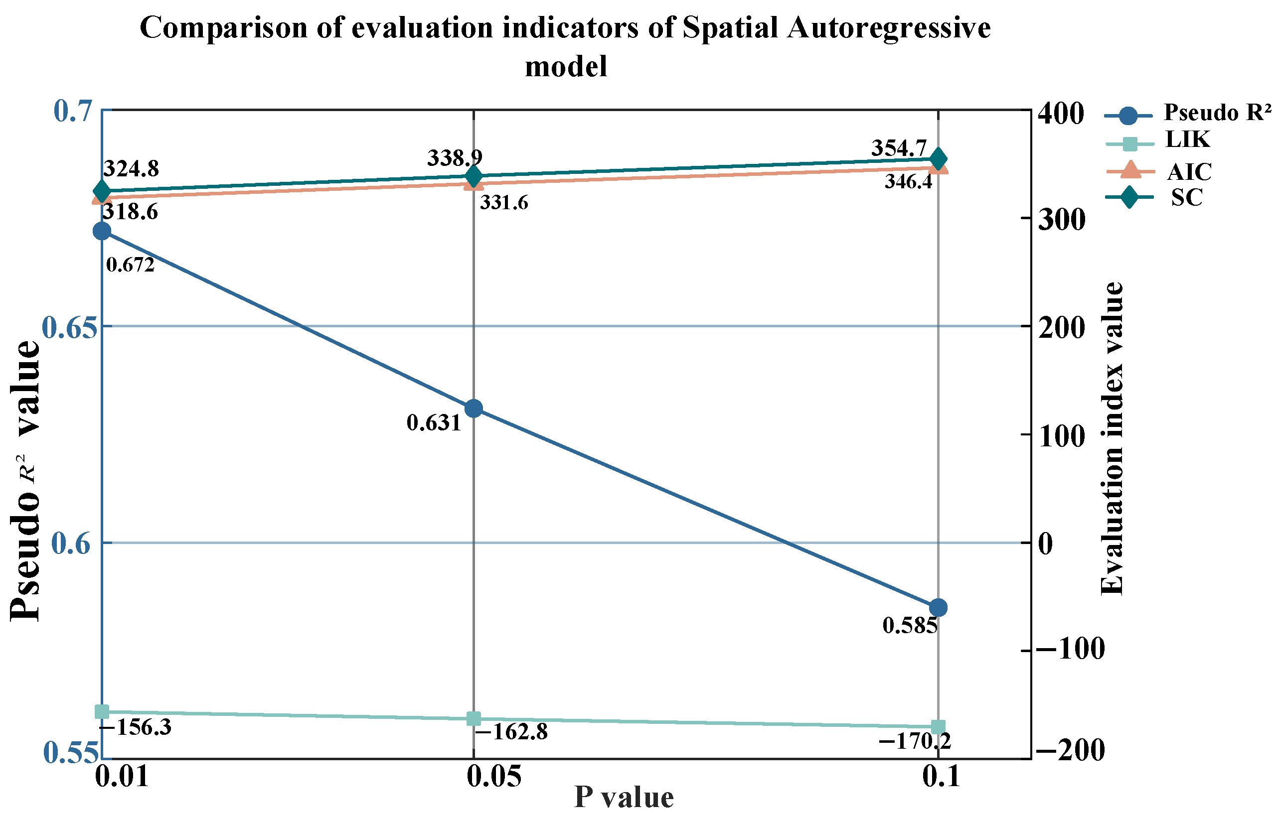
This paper analyzes the parameter estimation results of the SAR model through the maximum likelihood estimation method. It can be seen that when $\rho$ gradually increases from 0.01 to 0.1, each evaluation index of the model shows a significant changing trend; the pseudo $R^2$ value of the model drops significantly from the initial 0.45 to 0.32 (ρ = 0.05), and finally drops to 0.25 ($\rho$ = 0.1). This significant downward trend indicates that as the spatial correlation increases, the model’s explanatory ability for data variability weakens significantly. Meanwhile, the log-likelihood value (LIK) also shows a similar decreasing feature, gradually decreasing from 448 at $\rho$ = 0.01 to 425 at $\rho$ = 0.05, and finally dropping to 410 at $\rho$ = 0.1. This changing trend further confirms that a larger spatial correlation coefficient may not be conducive to the accurate estimation of model parameters.

In contrast, the indicators of the information criterion method show better stability: AIC and SC remain at the levels of 0.15 and 0.17, respectively, showing only a slight upward trend. This indicates that even when the spatial correlation changes, the model still maintains a good generalization ability and complexity balance. Among all parameter combinations, when $\rho$ = 0.01, the model exhibits the optimal comprehensive performance: it not only achieves the highest $R^2$ value (0.45) and LIK value (448) but also maintains relatively low AIC (0.15) and SC (0.17) values.

Based on the evaluation of various indicators, when the spatial autoregressive term is introduced, the SAR model outperforms the situation without introducing the spatial term in all indicators. This indicates that the DPFC communication delay is spatially interrelated, and the model achieves the optimal comprehensive performance when $\rho$ = 0.01. It is proved that a smaller spatial correlation coefficient is beneficial for the model to better capture the spatial dependency characteristics of the data. The specific parameter indicators are shown in Figure 4 below.

3.3. Comparative Analysis of the Solution Methods for the ARIMA-LSTM Hybrid Model

This study systematically evaluated two key integration methods of the ARIMA-LSTM hybrid model.

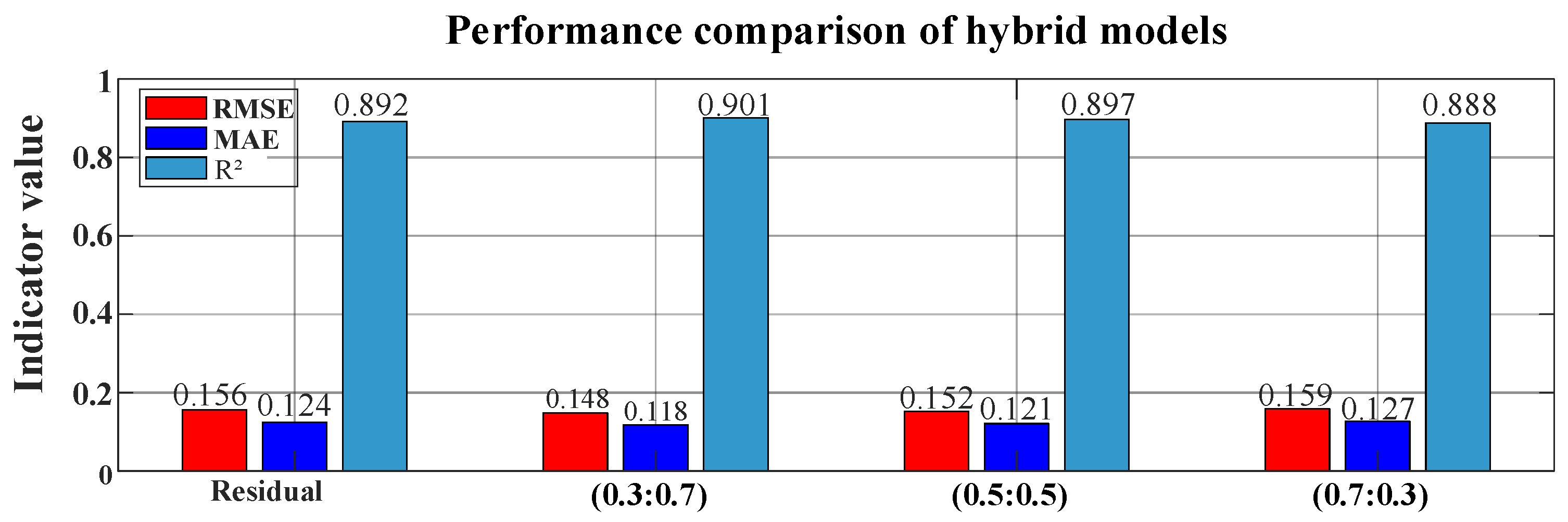
Method 1: by adopting the sequence mixing method based on residuals, relatively stable performance indicators were exhibited (RMSE = 1.56, MAE = 1.24, R = 8.92). Method 2: Model fusion is carried out through different weight combinations. Among them, the optimal effect is achieved when the weight ratio of ARIMA and LSTM is 0.3:0.7 (RMSE = 1.48, MAE = 1.18, R = 9.01), and there is a slight improvement in all indicators compared with Method 1. With the increase of the ARIMA weight, the model performance shows a downward trend. When the weight is 0.5:0.5 (RMSE = 1.52, MAE = 1.21, R = 8.97) and 0.7:0.3 (RMSE = 1.59, MAE = 1.27, R = 8.88), the prediction accuracy gradually decreases. This indicates that in this prediction task, the ability of LSTM to capture nonlinear features plays a more important role. Although the weighted mixing method with a weight of 0.3:0.7 can achieve slightly better performance, considering the stability of the model, computational efficiency, and the requirements of practical engineering applications, the sequence mixing method based on residuals has significant advantages, as follows: (1) no complex parameter tuning process is required, reducing the computational complexity; (2) it has stronger generalization ability and shows stability to different datasets. Figure 5 shows the performance comparison of the two hybrid methods under different parameter configurations.

3.4. Analysis of the Prediction Results of the ARIMA-LSTM Hybrid Model

In this section, we predict the communication delays of five DPFC devices. For the ARIMA model, the parameters (p, d, q) are selected according to the Akechi information criterion. Select triples (2,1,2) as the parameters (p, d, q) of the ARIMA model. When the ARIMA model conducts data prediction, it often has strict requirements for data stability. However, network latency is generally bursty. Therefore, differential operations need to be performed on the training set data first. The specific effect is shown in Figure 6 below.

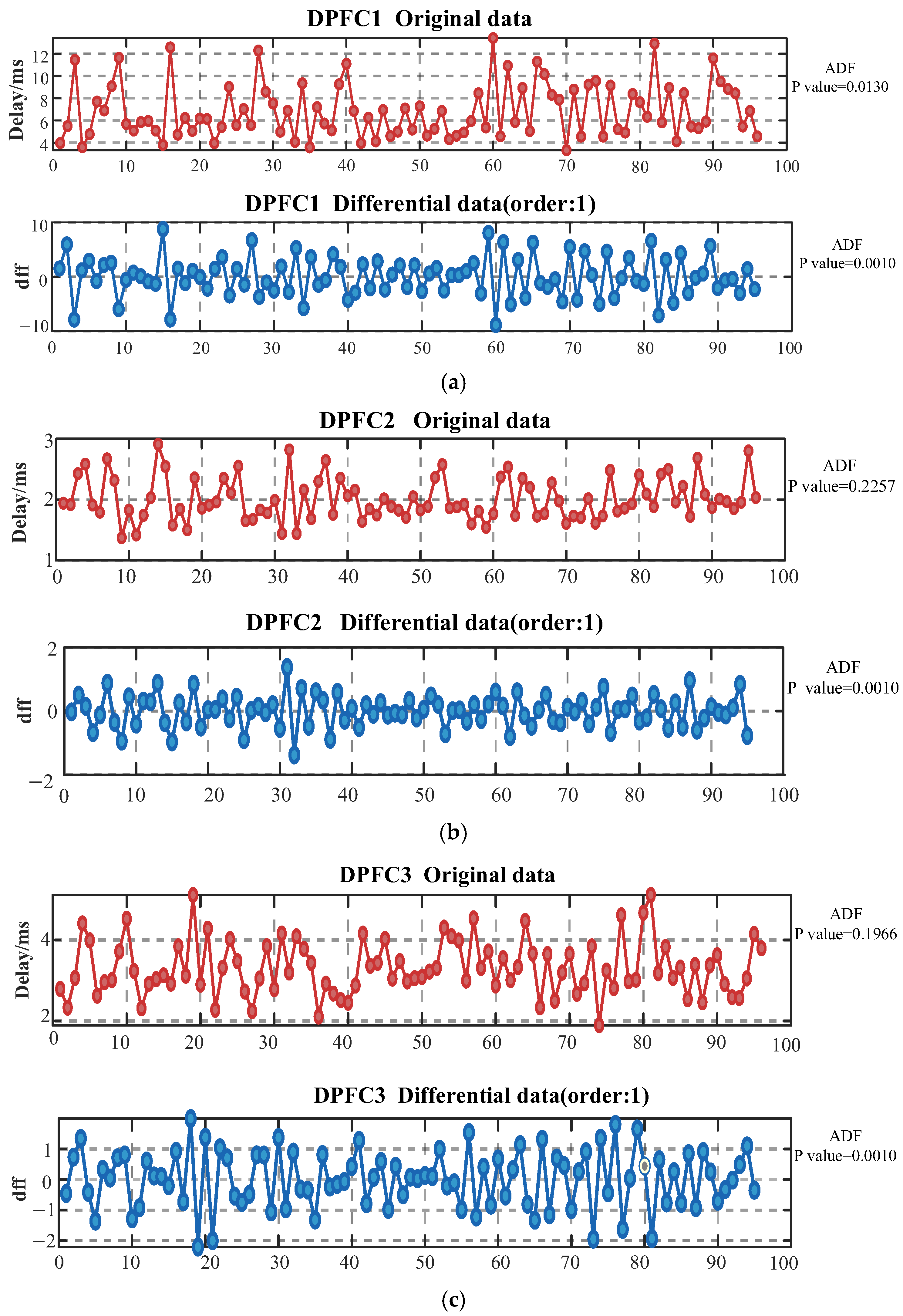
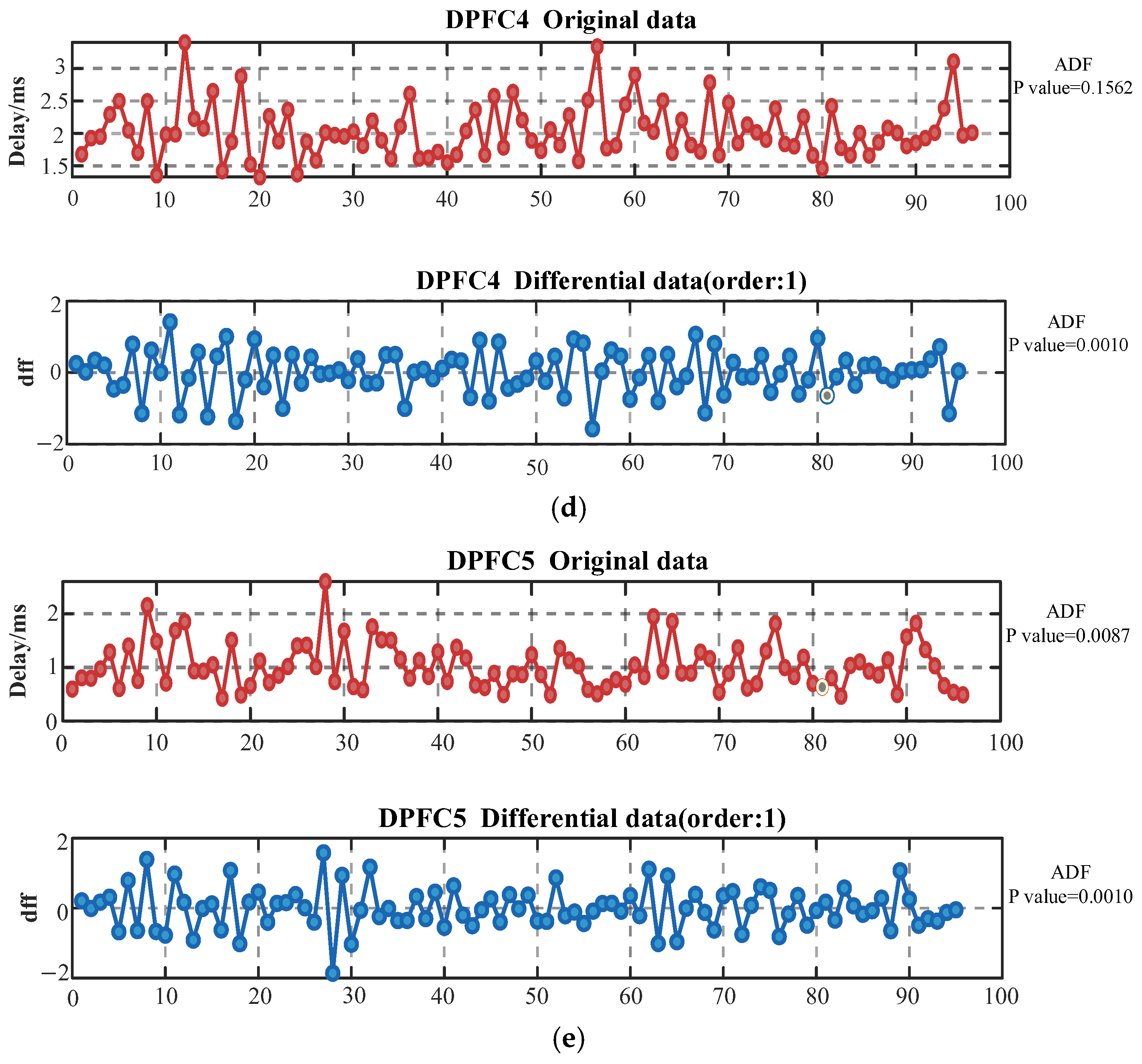
Through the analysis of the communication delay data of five DPFC devices, it can be seen that the original data all exhibit unstable characteristics to varying degrees. Among them, the fluctuation amplitude of DPFC1 is the largest (4–12 ms), and there are obvious sudden peaks. DPFC2 shows a relatively gentle fluctuation characteristic (1–3 ms) and has certain periodic changes. The ADF values of the original data of DPFC3, DPFC4 and DPFC5 were 0.1966, 0.1562 and 0.0087, respectively, all showing significant instability characteristics, further proving the instability of their time series. The significant differences in delay characteristics among devices indicate that the network conditions in different regions vary greatly, further suggesting that the spatial characteristics of devices should be considered during prediction.

After performing first-order difference processing on all the data, the ADF test values of the five DPFC devices were effectively reduced to 0.0010, which was lower than the critical value of 0.05, indicating that the data had met the stationarity requirements required for time series analysis. Specifically, the fluctuation range of DPFC1 after differential narrowed to ±8 ms, the fluctuation of DPFC2 was controlled within ±1 ms, while the fluctuation amplitudes of DPFC3, DPFC4, and DPFC5 were all maintained at around ±2 ms and fluctuated near the zero value, basically eliminating the trend components in the original data.

This paper first predicts the communication delay without considering the spatial characteristics of the device. The prediction results are shown in Figure 7 below.

By comparing and analyzing the actual communication delay values of five DPFC devices and the prediction results of the AMI-LSTM hybrid model, this study finds that this model shows a certain predictive ability without considering the spatial characteristics, but at the same time, there are significant limitations. The specific analysis is as follows:

The prediction deviation of DPFC1 in the delay peak range (8–12 ms) is relatively large. Especially when there are sharp fluctuations in the time series, the dynamic tracking ability of the model is significantly limited. Although the overall fluctuation of DPFC2 is relatively small (1.4–3 ms), and the prediction curve can basically track the changing trend of the actual value, it still has deficiencies in capturing local details. The prediction results of DPFC3 fluctuate within the range of 2.5–4 ms, and the fit with the actual values is relatively good, but there is a slight lag in the response to some mutation points. The prediction results of DPFC4 and DPFC5 also exhibit similar characteristics, namely, insufficient adaptability to rapid fluctuations within a short period of time.

Combined with the analysis of the previous data preprocessing, it can be found that although differential processing improves the robustness of the data (the ADF values of all DPFC are reduced to 0.0010), due to the neglect of the spatial correlation between DPFC (such as the optimal model performance when ρ = 0.01 is analyzed in the previous text), this leads to the model’s inability to fully utilize the mutual influence relationship among devices to improve the prediction accuracy, which indicates that the ARIMA-LSTM hybrid model that only relies on the characteristics of the time series has certain limitations.

3.5. Analysis of the Prediction Results of the Hybrid Model with Spatial Characteristics Introduced

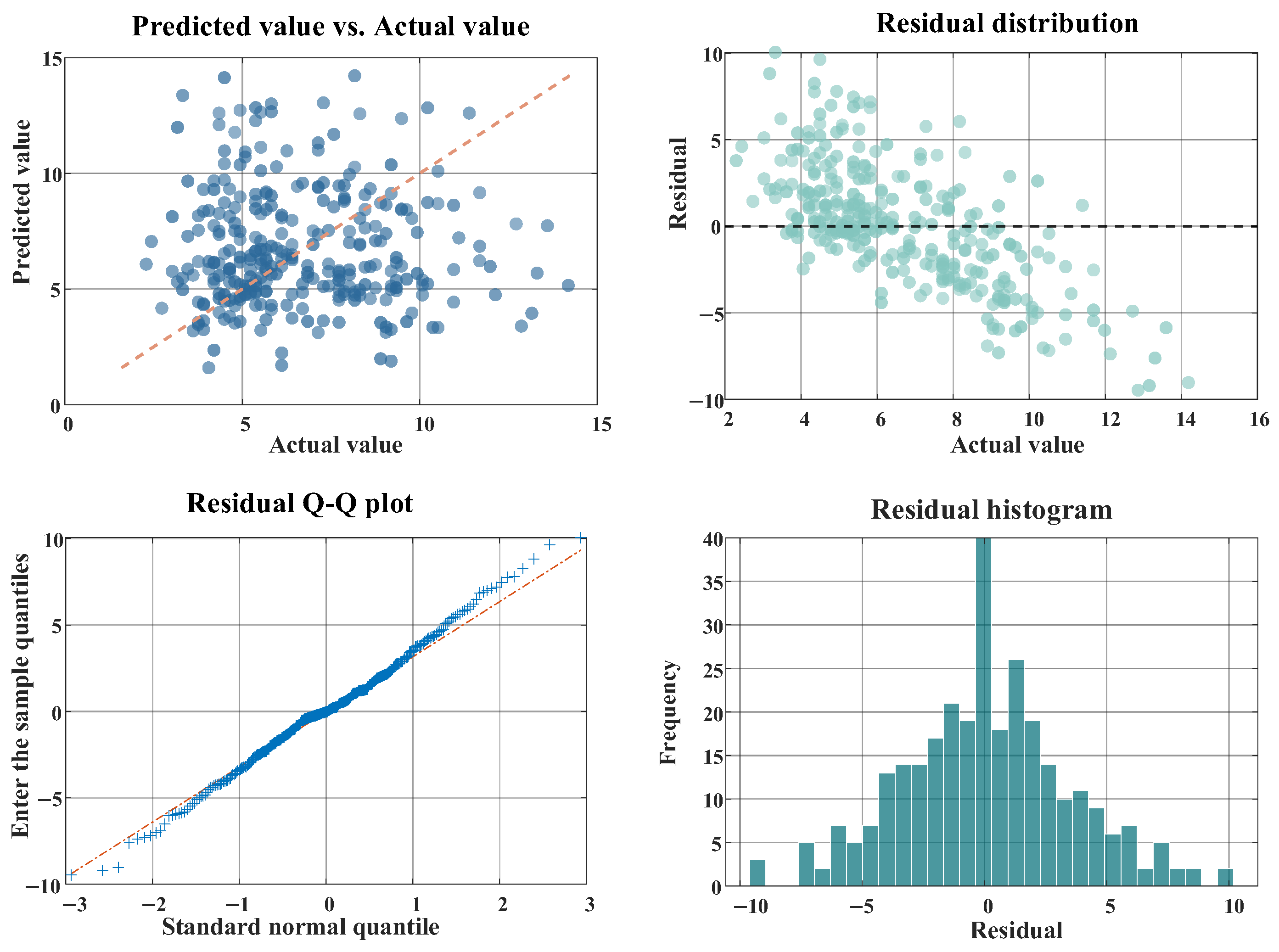
To comprehensively evaluate the prediction performance of the hybrid model after introducing spatial characteristics, this section conducts a detailed analysis from three dimensions: prediction accuracy, residual analysis, and temporal characteristics [26]. Figure 8 shows the overall evaluation of the prediction results.

From the perspective of the overall prediction performance of the model, the scatter plots of the predicted values and the actual values are highly concentrated near the y = x diagonal, indicating that the prediction results have a strong correlation with the actual values. The quantitative evaluation indicators show that the RMSE of this model is 1.2791 and the MAE is 1.0811. The residual distribution map shows that most of the prediction errors are controlled within the range of (−5.5), and present good randomness without obvious systematic deviations. The data points in the residual Q–Q plot are closely attached to the diagonal, indicating that the residuals approximately follow a normal distribution, which verifies the rationality of the model assumptions. The residual histogram shows obvious bell-shaped distribution characteristics, further confirming the normality of the model residuals and indicating that the model has well captured the main features of the data.

Figure 9 presents in detail the specific prediction effects of the five DPFC devices after introducing spatial characteristics. Through the local magnification analysis of the 200th–250th sample interval, the error between the predicted value and the actual value can be seen more intuitively.

Through a systematic evaluation of the prediction performance of each DPFC device, the analysis of each DPFC in this study includes a time series comparison chart and a sample distribution comparison chart. The experimental results show that DPFC1 demonstrates excellent tracking ability within a large fluctuation range (2–12 ms), that is, its prediction curve can capture the extreme value characteristics of sudden high delay to a limited extent. The comparison of sample distributions indicates that the distributions of predicted values and actual values in each interval are highly consistent. The delay fluctuation of DPFC2 is relatively small, and its prediction curve can accurately reflect this small oscillation characteristic. Especially in the main fluctuation range, the distribution of predicted values almost coincides with the actual values. The prediction results of DPFC3 show good adaptability to medium-scale fluctuations. The prediction curves in the time series graph accurately track the changing trend of the actual values, verifying the model’s ability to grasp medium-scale fluctuations. The prediction effects of DPFC4 and DPFC5 are equally satisfactory. Especially when dealing with rapid fluctuations and sudden changes, the prediction curves can respond promptly and track accurately. Compared with the prediction results without considering the spatial characteristics, the prediction performance after introducing the SAR model has been significantly improved. The prediction accuracy of sudden delay peaks has increased, the co-variation characteristics among multiple DPFCS have been better characterized, and the smoothness and continuity of the prediction curve have been improved. The introduction of the spatial autoregressive model SAR model for the limited capture of the spatial dependency relationship between DPFC devices improves the communication delay prediction effect of the devices. It can be known from the spatial correlation analysis in the previous text that although there is a relatively weak spatial correlation among the devices (optimal ρ = 0.01), after adding this correlation to the prediction framework, the model performance has been significantly improved. This result not only verifies the necessity of considering spatial characteristics but also provides a more reliable technical solution for communication delay prediction in practical engineering applications.

4. Conclusions

This study proposes a communication delay prediction method based on SAR-ARIMA-LSTM. By introducing the spatial autoregressive (SAR) model, the spatial dependence between DPFC devices is effectively captured, significantly improving the prediction accuracy. The research results show that spatial characteristics play an important role in communication delay prediction. This conclusion can be verified from the following aspects:

(1)

The results of spatial autoregressive analysis show that although there is a weak spatial correlation among DPFC devices (the optimal spatial correlation coefficient ρ = 0.01), this correlation is statistically significant. When the spatial correlation coefficient ρ = 0.01, the model achieves the best comprehensive performance: the pseudo $R^2$ value reaches 0.45, and the log-likelihood value (LIK) is 448, while maintaining a relatively low AIC (0.15) and SC (0.17) values. This indicates that even a relatively weak spatial dependency can provide valuable information for the prediction model.

(2)

By comparing the prediction results before and after adding spatial characteristics, the improvement in prediction accuracy can be clearly seen. When spatial characteristics are not considered, the model’s predictive ability for sudden delay peaks is limited, especially showing obvious limitations in the high delay interval (8–12 ms) of DPFC1 and the small fluctuation interval (1.4–3 ms) of DPFC2. After introducing spatial characteristics, the predictive ability of the model has been comprehensively enhanced. The RMSE has decreased to 1.2791, and the MAE has decreased to 1.0811. The scatter plots of the predicted values and the actual values are more concentrated near the ideal diagonal, and the residual distribution is also closer to the normal distribution.

(3)

From the perspective of temporal characteristics, the model with the addition of spatial characteristics shows stronger adaptability. Take DPFC1 as an example. The model can accurately capture large fluctuations within the range of 2–12 ms. Even when there is a sudden high delay of more than 10ms, the prediction curve can still maintain good tracking performance. This improvement has been reflected in the prediction results of all DPFC devices, indicating that the introduction of spatial characteristics effectively enhances the model’s ability to handle fluctuations of different scales.

However, there are still some directions worth of further exploration in this study, as follows:

(1)

The construction method of the spatial weight matrix can be further optimized. The currently adopted weight calculation method based on distance may not fully reflect the actual mutual influence relationship between DPFC devices. The multi-dimensional weight construction method considering factors such as equipment importance and load level is worth exploring.

(2)

There is still room for improvement in the real-time performance and computational efficiency of the model. Although the introduction of spatial characteristics improves the prediction accuracy, it also increases the computational complexity. In practical applications, a better balance point needs to be found between prediction accuracy and computational efficiency.

(3)

The model’s ability to handle extreme situations still needs to be strengthened. Although the current model can handle conventional fluctuations relatively well, for rare cases of extremely large delays or simultaneous mutations in multiple DPFCS, the prediction performance may not be ideal enough.

To sum up, this study has demonstrated the necessity and effectiveness of incorporating spatial characteristics into the prediction framework. By capturing the spatial dependency relationship through the SAR model and combining the linear prediction ability of the ARIMA model and the nonlinear feature extraction ability of LSTM, a more complete and accurate prediction system has been constructed. This method not only provides more reliable communication delay prediction results but also offers an important reference for the optimization of communication networks and the formulation of dispatching strategies in distributed power systems. Future research can focus on the directions discussed above to further enhance the performance and practicability of the model.