Evolutionary Framework with Binary Decision Diagram for Multi-Classification: A Human-Inspired Approach

Abstract

Current mainstream classification methods predominantly employ end-to-end multi-class frameworks. These approaches encounter inherent challenges including high-dimensional feature space complexity, decision boundary ambiguity that escalates with increasing class cardinality, sensitivity to label noise, and limited adaptability to dynamic model expansion. However, human beings may avoid these mistakes naturally. Research indicates that humans subconsciously employ a decision-making process favoring binary outcomes, particularly when responding to questions requiring nuanced differentiation. Intuitively, responding to binary inquiries such as “yes/no” often proves easier for humans than addressing queries of “what/which”. Inspired by the human decision-making hypothesis, we proposes a decision paradigm named the evolutionary binary decision framework (EBDF) centered around binary classification, evolving from traditional multi-classifiers in deep learning. To facilitate this evolution, we leverage the top-N outputs from the traditional multi-class classifier to dynamically steer subsequent binary classifiers, thereby constructing a cascaded decision-making framework that emulates the hierarchical reasoning of a binary decision tree. Theoretically, we demonstrate mathematical proof that by surpassing a certain threshold of the performance of binary classifiers, our framework may outperform traditional multi-classification framework. Furthermore, we conduct experiments utilizing several prominent deep learning models across various image classification datasets. The experimental results indicate significant potential for our strategy to surpass the ceiling in multi-classification performance.

1. Introduction

Classification tasks play a pivotal role in the field of deep learning, particularly in image classification, with applications spanning healthcare, public safety, and intelligent transportation, among others. As image classification technology continues to advance, supervised single-label closed-set classification tasks based on representative datasets such as CIFAR-10, CIFAR-100, and ImageNet have established fundamental benchmarks. In the pursuit of achieving superior performance on these datasets, researchers have explored various strategies including data preprocessing techniques, innovative model architectures, and the incorporation of additional information to enhance model performance. These strategies aim to leverage the powerful fitting capabilities of deep learning to learn more effective multi-class feature spaces. However, these approaches appear to have reached a bottleneck when data availability is limited, as traditional multi-class classifiers aim to fit a better mapping from the pixel space of images to a more separable multi-class feature space. This paradigm has some inherent problems including high-dimensional feature space complexity, decision boundary ambiguity that escalates with increasing class cardinality, sensitivity to label noise, and limited adaptability to dynamic model expansion.

Observing the human decision-making process in object classification, we have identified that the abstraction process of “multi-class classification” can be reframed as a simpler question: “To which category does this object belong among all available categories?” In contrast, it is much easier for humans to answer questions like “Does this image contain a cat?” or “Is this picture of cat?”. As shown in the Figure 1, we conducted an experiment to compare different questioning approaches. Clearly, questions presented in a binary form are significantly easier to answer. Furthermore, task difficulty escalated markedly with an increase in the number of response options provided in ‘which’-format questions. This phenomenon is similarly reflected in the decision-making framework of deep learning models, which are confined to applying parallel multi-class logic for decision-making.

Considering the human tendency to use binary decision-making in object classification, we revisited traditional binary classification strategies and recognized their advantages in classification tasks. Although early studies implemented multi-class classification through “one-vs-rest” (OVR) and “one-vs-all” (OVA) classifers, strategies employing voting over these binary classifiers have been widely recognized as significantly inferior to naive multi-class classification approaches. Although discrete binary classifiers significantly outperform multi-class classifiers on the recall metric (fig), we observe that a decision-making ‘gap’ persists by a process of “voting” on binary classifiers to deriving optimal multi-classification outcomes. Specifically, analogous to human cognition where distinct candidate categories warrant differential treatment, the subconscious ‘hierarchical’ inherent in human cognition may hold the key to achieving the transition from discrete binary classification to multi-class categorization.

To technically realize this process, we propose embedding the binary classification decision-making process into the multi-class decision-making framework and combining the results of multi-class classifiers to form a chained decision-making process. This strategy not only achieves a mapping from multi-class space to binary classification space but also enhances the interpretability of the decision-making process. Through experiments, we have validated the effectiveness and performance of the proposed method, offering a new perspective for future multi-class classification tasks by effectively combining the strengths of deep learning with traditional machine learning to help classifiers achieve better classification capabilities.

2. Related Work

2.1. Evolution of Multi-Class Classification

Deep learning methods for multi-class classification originated from adaptations of approaches initially designed for binary classification. Early techniques extended binary classifiers such as one-vs-rest (OvR) and one-vs-one (OVO), offering solutions to handle numerous classes or imbalanced data despite challenges including conflicting decisions and the requirement for multiple classifiers [1]. The field progressed with inherently multi-class algorithms like structured-output SVMs that optimize outcomes across all classes simultaneously [2,3], alongside probability adjustment techniques including Platt scaling [4] and tree-based methods such as random forests [5]. The deep learning revolution commenced with CNNs learning features directly from data [6], followed by architectures addressing challenges like vanishing gradients (e.g., ResNet, DenseNet) and maintaining spatial consistency in feature recognition [7]. Recent advances focus on efficiency, explainability, and reliability: Methods such as Motif-SET reduce parameters by 90% while retaining accuracy exceeding 96% through optimized network design [8]; attention mechanisms emphasize class-relevant features, demonstrated in cross-attention transformers for fine-grained recognition [9,10]; explainable systems integrate interpretability directly into architectures, exemplified by NSR-Net’s imaging modules [11] and concept bottleneck models with transparent intermediate features [12]; combined vision–language approaches like VILA-M3 align medical imagery with textual data [13] while MedUnifier bridges visual elements with linguistic understanding [14]; and reliability enhancements incorporate formal performance guarantees [15] and noise-resistant designs leveraging class relationships [16]. Collectively, these innovations significantly enhance performance, efficiency, and practical applicability across domains ranging from edge computing to healthcare diagnostics.

2.2. Rediscovery of Binary Classification Strategies

Binary classifiers, particularly one-vs-all (OVA) methods, have garnered renewed interest due to their alignment with human “yes or no reasoning” patterns and superior adaptability to real-world scenarios. While early OVA implementations using SVMs underperformed in deep learning contexts, recent studies demonstrate that deep OVA classifiers achieve higher recall rates in critical applications such as medical diagnosis and fraud detection, where explicit modeling of asymmetric misclassification costs is essential—for instance, overlooking a malignant tumor incurs substantially higher societal cost than false alarms [17]. This resurgence stems from three principal factors. Theoretical robustness of binary decomposition: Techniques like error-correcting output codes (ECOC) provide a principled framework for integrating binary classifiers with error-correction capabilities, enhancing resistance to label noise and data perturbations [18]. Hierarchical decision efficiency: Taxonomic organization of classes through binary trees reduces inference complexity in large-scale systems, evidenced by adaptive inference graphs that dynamically route samples to specialized binary sub-classifiers [19]. Optimization for class imbalance: Innovations such as focal loss dynamically adjust weights for challenging samples during training [20], while label over-smoothing (LOS) mitigates head-class dominance by softening inter-class boundaries in long-tailed data—achieving state-of-the-art results on ImageNet-LT and iNaturalist2018 through balanced prediction distributions across categories [21]. Furthermore, embedded feature selection techniques incorporate L1-norm penalties within binary classifiers to eliminate irrelevant features under noisy data conditions, enhancing model interpretability and resilience [22]. These advancements culminate in hybrid frameworks, like cost-sensitive deep OVA, that now surpass monolithic multi-class models by over 4.2% for recall in fine-grained recognition [9] and 3.7% for F1-score in medical imaging [14]. By leveraging the proven capabilities of binary learners and their intrinsic compatibility with human decision logic, binary-based methodologies retain significant potential for continued advancement.

2.3. Hybrid Decision Frameworks

The integration of multi-class and binary classifiers has emerged as an effective paradigm for balancing holistic context comprehension with localized decision precision, with recent advances enhancing static architectures through dynamic joint optimization. Early hierarchical CNNs decomposed complex tasks via coarse-to-fine feature abstraction [23], while adaptive inference graphs enabled sample-specific routing to specialized binary sub-classifiers [24]. Subsequent innovations integrated rule-based systems with deep features for interpretable predictions [25] and leveraged semantic hierarchies for scalable object detection [26]. Addressing the limitations of fixed architectures, advancements introduced three key developments. Zhang et al. developed cross-attention transformers performing initial coarse categorization followed by binary verification modules for ambiguous classes, reducing computational costs by 40% while maintaining an 86.4% accuracy on fine-grained tasks [9]. MedUnifier unified visual components with linguistic pretraining, utilizing multi-class vision modules for anatomical localization and binary classifiers for pathological-textual consistency verification, improving medical report accuracy by 3.7% for F1-score [14]. Nie et al. implemented topological sparsification within hybrid MLPs, eliminating 90% of parameters while preserving a >96% accuracy through the strategic pruning of auxiliary binary classifiers [8]. Theoretical advancements formalize these approaches: DecisionFlow structures decisions as differentiable graphs, converting multi-class predictions into binary action filters for resolving ethical dilemmas in critical scenarios—demonstrated by elevating GPT-4o’s diagnostic accuracy by 46% in low-utility contexts [27], while HybridFlow decouples decision logic from computational operations via its 3D-HybridEngine, enabling optimized resource allocation between multi-class generators and binary RLHF critics [28]. These hybrid systems demonstrate superiority over monolithic models through intelligent resource utilization: Global multi-class layers preserve holistic context [29], while focused binary classifiers resolve uncertainties using human-aligned reasoning.

3. Methods

3.1. Problem Statement

3.1.1. Analysis of Multi-Class Classifier Decision Patterns

The decision-making process of traditional deep learning-based multi-class classifiers can be succinctly characterized as follows: For an input sample, the classifier assigns confidence scores to all candidate categories, then ranks these scores in descending order. The category with the highest score (Top-1 prediction) is selected as the final prediction. This prediction is compared against the ground-truth label to determine correctness—correct if matched, incorrect otherwise. However, our empirical analysis reveals a significant phenomenon: Among samples misclassified by the Top-1 criterion, the majority (typically >65%) retain their true labels within the Top-5 predicted categories [30].

This observation is quantitatively substantiated by evaluating mainstream deep learning architectures across benchmark datasets. As demonstrated in

Table 1. Top-1 vs. Top-5 accuracy of mainstream models (%).

Model	Dataset	Top-1	Top-5	Gap
ResNet-152	ImageNet	76.0	93.0	17.0
EfficientNet-B7	ImageNet	84.4	97.1	12.7
ViT-L/16	ImageNet	88.9	98.7	9.8
DenseNet-201	CIFAR-100	77.3	94.2	16.9
Inception-v4	Birdsnap	73.8	92.6	18.8

, even non-state-of-the-art models exhibit substantial performance gaps between Top-1 and Top-5 accuracy. For instance, ResNet-152 achieves 76.0% Top-1 accuracy on ImageNet, while its Top-5 accuracy reaches 93.0%—indicating that 17% of samples misclassified under Top-1 criterion have correct labels captured in the extended Top-5 set [30]. Similarly, DenseNet-201 shows a 16.9% accuracy gap on CIFAR-100, confirming the pervasiveness of this pattern across data domains.

For samples misclassified by the multi-class classifier, we randomly selected instances from CIFAR-100 and retrieved their prediction trajectories within the classifier. As shown in Figure 2, we observed that the ground-truth labels of many misclassified samples were actually exhibited in the classifier’s top-5 predictions. This finding aligns with the previously discussed conclusion. Furthermore, when we processed these misclassified samples using their corresponding binary classifiers, we found that the binary classifiers could typically achieve correct predictions with relative ease. This highlights why effectively utilizing the complementary strengths of the top-5 predictions and the binary classifiers became the core objective of our research.

3.1.2. Binary Classification Is Easier than Multi-Classification

Intuitively, binary classification entails simpler decision boundaries, rendering it easier compared to multi-class classification. Figure 3 below illustrates the true positive rate (TPR) for each class corresponding to multi-class and binary classifications on the CIFAR-100 dataset. On average, the TPR level for binary classifiers exceeds that of multi-class classifiers. This suggests that binary classifiers may correctly identify samples that are misclassified by multi-classification.

Based on the TPR analysis, binary classification appears to surpass multi-class classification. However, this comparison may not be entirely equitable. This is due to the inherent limitation of discrete binary classifiers, which cannot inherently handle multi-class decisions. The simple voting strategy incurs a steep degradation in classification performance exponentially. To address this limitation within multi-class classification tasks, we propose a method for integrating binary classification into a multiclass framework. This method involves evolving the multi-class space into a final binary classification space to enhance decision-making. In the subsequent section, we will elaborate on this methodology. Furthermore, we visualize the CAM (class activation mapping) heatmaps for both the multi-class and binary classifiers in Figure 4, ensuring controlled variables such that both models were trained on identical data. The results demonstrate that for samples correctly classified by both classifiers, the binary classifier exhibits more precise localization within its regions of interest. Crucially, for instances where the multi-class classifier makes an error while the binary classifier classifies correctly, as shown in Figure 4b,c, the binary classifier consistently focuses on discriminative regions relevant to the target class. For example, for the “cloud” class, the multi-class classifier correctly highlights the location of clouds in the sky region. However, for distinguishing the “boy” class, the binary classifier effectively concentrates on facial features critical for the boy/girl distinction, enabling its correct classification.

3.1.3. Notion Definition

For a closed-set multi-classification task, let the target set be $\mathcal{Y}=\{0,1,\dots ,N-1\}$. Considering binary classification, define a binary target set for the i-th class as $\mathcal{S}=\{0,1\}$, where $i\in \mathcal{Y}$. For a class y in $\mathcal{Y}$, we expect to obtain such a mapping $g_{\mathrm{s}}^{(Bi)}:\mathcal{Y}\to \mathcal{S}$ based on a binary classifer $Bi$ defined as

$$\begin{array}{c}\hfill g_s^{(Bi)}=\left\{\begin{array}{cc}0,\hfill & \mathrm{if}y=i,\hfill \\ 1,\hfill & \mathrm{if}y\ne i.\hfill \end{array}\right.\end{array}$$

(1)

Here, i represents the i-th component in the original target set $\mathcal{Y}$, and s represents an instance in the set $\mathcal{S}$. More specifically, when we get a sample x in $\mathcal{X}=\{0,1,\dots ,K-1\}$, there exist a mapping $f_y^{(M)}(x):\mathcal{X}\to \mathcal{Y}$ defined for multi-classification based on multi-class classifier M. Correspondingly, we propose the following equation to get a final mapping:

$$\begin{array}{c}\hfill g_s[f_y^{(Bi)}(x)]:\mathcal{X}\to \mathcal{S},\end{array}$$

(2)

which is our binary learning framework designed for binary classification. In the next section, we propose a possible concrete strategy to realize this transformation of the classification space and the final decision.

3.2. Methodology

We propose an evolutionary strategy that transforms the final decision-making process into a binary one. As formalized in Equation (2), our strategy identifies the class i when $g_s[f_y^{Bi}(x)]=0$ through a chained approach leveraging binary classification outcomes. The complete procedure is detailed in Algorithm 1.

Algorithm 1 Binary Learning Strategy for Multi-classification.
1:	Require: Set of N categories $\mathcal{Y}=[0,1,\dots ,N-1]$, binary classifiers $\{B_0,B_1,\dots ,B_{N-1}\}$, multiclass classifier M, sort function $rank()$
2:	Input: x (sample), $\{B_i\}$, M
3:	Output: Predicted class y
4:	$i\leftarrow 0$, $\mathcal{R}\leftarrow \mathcal{Y}$, $d\leftarrow 1$
5:	$\mathcal{R}\leftarrow rank(M(x))$	Sort classes by M’s confidence
6:	while $i<N$ do
7:	$d\leftarrow B_{\mathcal{R}[i]}(x)$	Query binary classifier
8:	if $d=0$ then return $\mathcal{R}[i]$	Terminate on first positive
9:	$i\leftarrow i+1$

This strategy operates by first embedding sample x using multi-class classifier M, which scores candidate classes in $\mathcal{Y}$ and sorts them in descending confidence order. Binary classifiers $\{B_i\}$ are then sequentially invoked until one returns “yes” (0), with termination upon the first positive identification. Crucially, performance degradation scales with the number of binary invocations per sample. However, as established in prior analysis, correct labels typically reside in the Top5 predictions, substantially reducing invocation costs.

The approach better leverages binary classifiers’ advantages, yielding higher prediction confidence. Figure 5 illustrates this through accuracy–confidence relationships, showing EBDF (green/orange/yellow) outperforming standalone classifiers (blue), with proximity to the top-right indicating optimal performance.

Not all EBDF enhance performance equally. Binary classifier accuracy proves more influential than other factors (baseline classifier performance or classifier independence), as formalized in Proof of Superior Performance Section. We subsequently establish theoretical conditions where our framework exceeds traditional multi-class approaches.

3.3. Theoretical Analysis

3.3.1. Each Step Error

As a multi-stage decision chain, the EBDF strategy implements sequential decisions to minimize the global error rate. The global error rate is accumulated from minor errors at each decision step by binary classifiers. However, conventional error rate metrics fail to quantify how localized errors propagate through the structured decision framework in EBDF. To address this limitation, we propose the progressive step-wise error rate (PSER), defined as

$${\mathrm{PSER}}^{(k)}={\displaystyle \frac{E^{(k)}}{N_{\mathrm{remaining}}^{(k-1)}}},$$

(3)

where $E^{(k)}$ denotes the number of erroneously processed samples at the k-th decision step, and $N_{\mathrm{remaining}}^{(k-1)}$ represents the total number of unresolved samples carried forward from the preceding $k-1$ steps.

This metric uniquely quantifies the conditional probability of decision errors relative to the actionable sample pool at each step. Unlike static error rates that normalize errors against fixed denominators such as the total initial samples, PSER adaptively weights errors by $1/N_{\mathrm{remaining}}$, thereby amplifying the significance of errors occurring in later stages where $N_{\mathrm{remaining}}$ diminishes. This dynamic scaling ensures that the metric maintains theoretical consistency with the step-wise decision framework while preserving practical interpretability across all stages, even as $N_{\mathrm{remaining}}$ progressively contracts.

In the EBDF framework, the progressive step-wise error rate (PSER) serves as a novel metric for quantifying discrepancies between binary decisions and traditional multi-classification outcomes. As illustrated in Figure 6, we formally define sample categories at each decision stage to compute stage-specific PSER values.

The partial stepwise error rate (PSER) for the baseline model is defined as

$${\mathrm{PSER}}_B^{(1)}={\displaystyle \frac{F_B^{(1)}}{T_B^{(1)}+F_B^{(1)}+N_r^{(1)}}}.$$

(4)

For cases where $T_M+F_M\ne 0$, we define the precision-enhanced recognition efficiency (PERE) as

$${\mathrm{PERE}}_M^{(1)}:={\displaystyle \frac{T_M}{T_M+F_M}}.$$

(5)

Regarding the error rate analysis, according to the sample types described in the figure, we can calculate PSER for both approaches. For traditional multi-class classification with single-step decision making, the one-step error rate is equivalent to the conventional error rate, expressed as

$${\mathrm{PERE}}_M^{(1)}:={\displaystyle \frac{T_M}{T_M+F_M}}.$$

(6)

For the EBDF method, the error rate at each decision step is analyzed as follows. At step 1, the PSER is given by

$${\mathrm{PSER}}_B^{(1)}={\displaystyle \frac{F_B^{(1)}}{T_B^{(1)}+F_B^{(1)}+N_r^{(1)}}}.$$

(7)

At step 2, it becomes

$${\mathrm{PSER}}_B^{(2)}={\displaystyle \frac{F_B^{(2)}}{N_r^{(1)}}}.$$

(8)

At step 3, the expression is

$${\mathrm{PSER}}_B^{(3)}={\displaystyle \frac{F_B^{(3)}}{N_r^{(2)}}}.$$

(9)

Finally, at step k for $k\in (1,N]$ with $N\in \mathbb{N}$, the generalized form is

$${\mathrm{PSER}}_B^{(k)}={\displaystyle \frac{F_B^{(k)}}{N_r^{(k-1)}}}.$$

(10)

3.3.2. Proof of Superior Performance

Under this framework, we demonstrate that each decision step in EBDF achieves significantly lower error rates than the single-step error rate of traditional multi-class classification. The proof proceeds as follows:

Step-1 Analysis

$${\mathrm{PSER}}_M^{(1)}={\displaystyle \frac{M·{\mathrm{PSER}}^{(1)}}{M}}>{\displaystyle \frac{P_B^{(1)}·e_M}{M}},$$

(11)

$${\mathrm{PSER}}_B^{(1)}={\displaystyle \frac{F_B^{(1)}}{M}}={\displaystyle \frac{P_B^{(1)}·e_B}{M}}.$$

(12)

Given ${\mathrm{e}}_{\mathrm{M}}>{\mathrm{e}}_{\mathrm{B}}$, we derive

$${\mathrm{PSER}}_M^{(1)}>{\mathrm{PSER}}_B^{(1)}.$$

(13)

Step-k Analysis (1 < k < N)

$${\mathrm{PSER}}_B^{(2)}={\displaystyle \frac{F_B^{(2)}}{N_r^{(1)}}}={\displaystyle \frac{F_B^{(2)}}{M}}·{\displaystyle \frac{M}{N_r^{(1)}}}<{\displaystyle \frac{F_B^{(2)}}{M}}·{\displaystyle \frac{M}{F_M^{(1)}}}.$$

(14)

The inequality $N_r^{(1)}>F_M^{(1)}$ holds because

$$\begin{array}{cc}\hfill F_M^{(1)}& =1-T_M^{(1)},\hfill \end{array}$$

(15)

$$\begin{array}{cc}\hfill N_r^{(1)}& =1-P_B^{(1)}=1-[(1-e_M)T_M^{(1)}]=1-T_M^{(1)}+e_M{T}_M^{(1)}.\hfill \end{array}$$

(16)

Therefore,

$${\mathrm{PSER}}_M^{(1)}={\displaystyle \frac{M{e}_M}{M}}={\displaystyle \frac{M{e}_M^2}{M{e}_M}}.$$

(17)

Given $P_B^{(2)}-P_B^{(1)}<M{e}_M$, we have

$$F_B^{(2)}=(P_B^2-P_B^{(1)})e_B<M{e}_M{e}_B.$$

(18)

Substituting into Equation (12) gives

$${\mathrm{PSER}}_B^{(2)}<{\displaystyle \frac{F_B^{(2)}}{M{e}_M}}={\displaystyle \frac{M{e}_M{e}_B}{M{e}_M}}<{\displaystyle \frac{M{e}_M^2}{M{e}_M}}={\mathrm{PSER}}_M^{(1)}.$$

(19)

• Statistical Validation

Through statistical analysis, we confirm that for existing methods when $k<6$, the inequality $M{e}_M>N_r^{(k)}$ consistently holds, thereby maintaining the validity of our conclusions. The complete derivation is omitted here for brevity.

• Verification with Experimental Data

Based on our experimental data, we calculated the EBDF and multi-classification PSER to facilitate a more intuitive demonstration of EBDF’s advantages. For the CIFAR100 dataset, the test set contains 10,000 images (i.e., M=10,000). The top-1 to top-5 accuracy rates using CLIP are 78%, 86%, 91%, 95%, and 98%, respectively.

Given the total sample size $M={10}^4$ and the single binary classifier error rate $e_r=3\%$, we construct the hierarchical error boundary decomposition framework (EBDF). The core algorithms are shown in Equations (1)–(3):

$$\Delta P^{(k)}=P_B^{(k)}-P_B^{(k-1)}(P_B^{(0)}=0),$$

(20)

$$\begin{array}{cc}\hfill T_B^{(k)}& =\Delta P^{(k)}\times (1-e_r),\hfill \end{array}$$

(21)

$$\begin{array}{cc}\hfill F_B^{(k)}& =\Delta P^{(k)}\times e_r,\hfill \end{array}$$

(22)

$$\begin{array}{cc}\hfill N_r^{(k)}& =M-P_B^{(k)}.\hfill \end{array}$$

(23)

By progressively decomposing the top-5 samples of the multi-classifier as $P^{(1)}$ to $P^{(5)}$, we obtain the calculation results, as shown in

Table 2. Layer parameter decomposition results.

Layer	$\Delta {\mathit{P}}^{(\mathit{k})}$	${\mathit{T}}_{\mathit{B}}^{(\mathit{k})}$	${\mathit{F}}_{\mathit{B}}^{(\mathit{k})}$	${\mathit{N}}_{\mathit{r}}^{(\mathit{k})}$
Top-1	7800	7566	234	2200
Top-2	700	679	21	1500
Top-3	600	582	18	900
Top-4	400	388	12	500
Top-5	300	291	9	200

:

Based on the PSER metric, calculate the residual error ratio for each layer:

$${\mathrm{PSER}}_B^{(k)}={\displaystyle \frac{F_B^{(k)}}{N_r^{(k-1)}}}(N_r^{(0)}=M).$$

(24)

$$\begin{array}{cc}\hfill \mathrm{Step}\text{-}1:& {\displaystyle \frac{234}{10000}}=2.34\%;\hfill \\ \hfill \mathrm{Step}\text{-}2:& {\displaystyle \frac{21}{2200}}\approx 0.95\%;\hfill \\ \hfill \mathrm{Step}\text{-}3:& {\displaystyle \frac{18}{1500}}=1.20\%;\hfill \\ \hfill \mathrm{Step}\text{-}4:& {\displaystyle \frac{12}{900}}\approx 1.33\%;\hfill \\ \hfill \mathrm{Step}\text{-}5:& {\displaystyle \frac{9}{500}}=1.80\%.\hfill \end{array}$$

For these five steps, calculate the average to obtain the average error rate:

$$\overline{{\mathrm{PSER}}_B}={\displaystyle \frac{1}{5}}{\displaystyle \sum _{k=1}^5}{\mathrm{PSER}}_B^{(k)}=1.52\%.$$

(25)

Compared to the global error rate ${\mathrm{PSER}}_M^{(1)}=22\%$ of the traditional multi-classifier, this method achieves an absolute reduction in the error rate from $22\%\to 1.52\%$ (a reduction of 93.1%) and an increase in the sample processing efficiency (the first three layers process 93.2% of the samples ($P_B^{(3)}=91\%$)).

3.4. Proof of the Condition That EBDF Works over Traditional Multi-Classification

3.4.1. Formalization of Confusion Probability Matrices

To rigorously characterize the probabilistic behavior of classification systems, we formalize three specialized confusion probability matrices as Figure 7:

• Confusion Probability Matrix for Multi-class Classifiers (PMMC): For a multi class model M trained on ${\mathcal{D}}_{\mathrm{r}}$, we define the probability set $\mathcal{C}=\{p_{m,n}^M\mid m,n\in \mathcal{Y}\}$ where

  $$p_{m,n}^M=P(\widehat{y}=n\mid y=m)\mathrm{and}{\displaystyle \sum _{n=0}^{\mathrm{N}-1}}{p}_{m,n}^M=1$$

  (26)
  Here, $p_{m,n}^M$ quantifies the probability that a sample with true class m is predicted as class n by M.
• Confusion Probability Matrix for Binary Classifiers (PMBC): For a binary classifier $B_i$ focused on class i, the probability set is ${\mathcal{B}}_i=\{p_{0,0}^{B_i},p_{0,1}^{B_i},p_{1,0}^{B_i},p_{1,1}^{B_i}\}$ with the constraints

  $$p_{0,0}^{B_i}+p_{0,1}^{B_i}=1\mathrm{and}{p}_{1,0}^{B_i}+p_{1,1}^{B_i}=1$$

  (27)

  where $p_{1,1}^{B_i}$ denotes the true positive rate for class i and $p_{0,0}^{B_i}$ the true negative rate.
• Score-Ordered PMMC (PMMC-DS): This matrix reindexes PMMC by sorting classes in descending order of model confidence scores. For a sample x, we define

  $${\mathcal{C}}^{\prime }=\{p_{{\mathrm{t}}_i,\widehat{{\mathrm{t}}_j}\mid {\mathrm{t}}_i,{\mathrm{t}}_j\in {\mathcal{Y}}_{\mathrm{sorted}}}^{M^{\prime }}\}$$

  (28)

  where ${\mathcal{Y}}_{\mathrm{sorted}}=\{{\mathrm{t}}_1,{\mathrm{t}}_2,\dots ,{\mathrm{t}}_{\mathrm{N}}\}$ with ${\mathrm{t}}_1$ being the top-predicted class, and ${\sum }_{j=1}^{\mathrm{N}}{p}_{{\mathrm{t}}_i,\widehat{{\mathrm{t}}_j}}^{M^{\prime }}=1$. This ordering enables position-aware probability analysis.

In our EBDF approach, in order to articulate the probability of all judgments being accurate, we employ PMMC-DS to segment the entire judgment process into N distinct events. The decision process is illustrated in Figure 8. The ultimate probability of accuracy is then the weighted aggregate of these individual events. These events are segmented based on the true labels occupying various ranking positions within the multi-classifier, as different rankings influence how binary classification is employed throughout the judgment process. Consequently, the probability associated with each event typically entails a series of interconnected operations. Figure 8 delineates the process of probability computation across different scenarios.

Figure 7. Probability confusion matrix for classifiers.

Figure 7. Probability confusion matrix for classifiers.

Figure 8. Confusion matrix visualization of EBDF decision process: (a) Step 1: top-1 classifier decision at $t_1$, (b) Step 2: top-2 classifier decision at $t_2$, (c) Step i: iterative decision optimization at $t_i$. Diagonal patterns indicate classification confidence levels.

Figure 8. Confusion matrix visualization of EBDF decision process: (a) Step 1: top-1 classifier decision at $t_1$, (b) Step 2: top-2 classifier decision at $t_2$, (c) Step i: iterative decision optimization at $t_i$. Diagonal patterns indicate classification confidence levels.

If the ground truth label ${\mathrm{t}}_1$ of sample x resides in the Top-1 of the score ranking from the multi-class classifier, the probability of the correct event is

$$\begin{array}{c}\hfill P_{\mathrm{T}}^{B_1}=p_{{\mathrm{t}}_1,{\widehat{\mathrm{t}}}_1}^{M^{\prime }}·p_{0,0}^{B{\mathrm{t}}_1},\end{array}$$

(29)

On the contrary, the probability of misclassification is

$$\begin{array}{c}\hfill P_{\mathrm{F}}^{B1}=p_{{\mathrm{t}}_1,{\widehat{\mathrm{t}}}_1}^{M^{\prime }}·(1-p_{0,0}^{B{\mathrm{t}}_1})+(1-p_{{\mathrm{t}}_1,{\widehat{\mathrm{t}}}_1}^{M^{\prime }}).\end{array}$$

(30)

In this strategy, merely applying our approach to the Top-1 scenario will not yield better results compared to standalone multi-classification, as $p_{{\mathrm{t}}_1,{\widehat{\mathrm{t}}}_1}^M>P_{\mathrm{T}}^{B_1}$. However, compared to the approach of multi-classification focusing on Top-1 judgment as $p_{{\mathrm{t}}_1,{\mathrm{t}}_1}^{M^{\prime }}$, employing a double check based on binary classification will lead to subsequent gains. The probabilities of these gain events occur in a chained formation. Additionally, as long as the subsequent probabilities satisfy ${\sum }_{i=2}^{\mathrm{N}}{P}_{\mathrm{T}}^{B_i}>p_{{\mathrm{t}}_1,{\widehat{\mathrm{t}}}_1}^{M^{\prime }}-P_{\mathrm{T}}^{B_1}$, our framework can achieve further performance evolution in the realm of multi-classification.

If the ground truth label ${\mathrm{t}}_2$ of sample x resides in the Top-2 of the score ranking from the multi-class classifier, the probability of the correct event is

$$\begin{array}{c}\hfill P_{\mathrm{T}}^{B_2}=p_{{\mathrm{t}}_2,{\widehat{\mathrm{t}}}_1}^{M^{\prime }}·p_{1,1}^{B{\mathrm{t}}_1}+p_{{\mathrm{t}}_2,{\widehat{\mathrm{t}}}_2}^{M^{\prime }}·p_{0,0}^{B{\mathrm{t}}_2},\end{array}$$

(31)

On the contrary, the probability of misclassification is

$$\begin{array}{cc}\hfill P_{\mathrm{F}}^{B_2}& =p_{{\mathrm{t}}_2,{\widehat{\mathrm{t}}}_1}^{M^{\prime }}·(1-p_{1,1}^{B{\mathrm{t}}_1})+p_{{\mathrm{t}}_2,{\widehat{\mathrm{t}}}_2}^{M^{\prime }}·(1-p_{0,0}^{B{\mathrm{t}}_2})+(1-p_{{\mathrm{t}}_2,{\widehat{\mathrm{t}}}_1}^{M^{\prime }}-p_{{\mathrm{t}}_2,{\widehat{\mathrm{t}}}_2}^{M^{\prime }}).\hfill \end{array}$$

(32)

For other more general cases, if the ground truth label ${\mathrm{t}}_{\mathrm{i}}$ of sample x resides in the Top-i ($i\le \mathrm{N}$) of the score ranking from the multi-class classifier, the probability of the correct event is

$$\begin{array}{cc}\hfill P_{\mathrm{T}}^{B_{\mathit{i}}}& =p_{{\mathrm{t}}_{\mathit{i}},{\widehat{\mathrm{t}}}_1}^{M^{\prime }}·p_{1,1}^{B{\mathrm{t}}_1}+p_{{\mathrm{t}}_{\mathit{i}},{\widehat{\mathrm{t}}}_2}^{M^{\prime }}·p_{1,1}^{B{\mathrm{t}}_2}+p_{{\mathrm{t}}_{\mathit{i}},{\widehat{\mathrm{t}}}_3}^{M^{\prime }}·p_{1,1}^{B{\mathrm{t}}_3}+\cdots +p_{{\mathrm{t}}_{\mathit{i}},{\widehat{\mathrm{t}}}_{\mathit{i}}}^{M^{\prime }}·p_{0,0}^{B{\mathrm{t}}_{\mathit{i}}},\hfill \end{array}$$

(33)

On the contrary, the probability of misclassification is

$$\begin{array}{cc}\hfill P_{\mathrm{F}}^{B_{\mathit{i}}}& =p_{{\mathrm{t}}_{\mathit{i}},{\widehat{\mathrm{t}}}_1}^{M^{\prime }}·(1-p_{1,1}^{B{\mathrm{t}}_1})+p_{{\mathrm{t}}_{\mathit{i}},{\widehat{\mathrm{t}}}_2}^{M^{\prime }}·(1-p_{1,1}^{B{\mathrm{t}}_2})+p_{{\mathrm{t}}_{\mathit{i}},{\widehat{\mathrm{t}}}_3}^{M^{\prime }}·(1-p_{1,1}^{B{\mathrm{t}}_3})+\cdots +\hfill \\ \hfill & p_{t_{\mathit{i}},{\widehat{t}}_{\mathit{i}}}^{M^{\prime }}·(1-p_{0,0}^{B{\mathrm{t}}_{\mathit{i}}})+(1-p_{{\mathrm{t}}_{\mathit{i}},{\widehat{\mathrm{t}}}_1}^{M^{\prime }}-p_{{\mathrm{t}}_{\mathit{i}},{\widehat{\mathrm{t}}}_2}^{{\mathrm{M}}^{\prime }}-p_{{\mathrm{t}}_{\mathit{i}},{\widehat{\mathrm{t}}}_3}^{M^{\prime }}-\cdots -p_{{\mathrm{t}}_{\mathit{i}},{\widehat{\mathrm{t}}}_{\mathit{i}}}^{M^{\prime }}).\hfill \end{array}$$

(34)

Accordingly, $\forall i\in \mathbb{Z},0<i\le \mathrm{N}{P}_{\mathrm{T}}^{B_i}+P_{\mathrm{F}}^{B_i}=1$.

Building upon the aforementioned derivation, we introduce some approximations and assumptions to facilitate clearer conclusions. Firstly, we assume that the true positive rate (TPR) and true negative rate (TNR) of the binary classifier are equivalent, denoted as $p_{0,0}^{Bi}=p_{1,1}^{Bi}=p_{\mathrm{b}}$. Additionally, we presume class balance and fairness in the model’s judgments across all classes, allowing each class ${\mathrm{t}}_{\mathrm{i}}$ to be uniformly sampled within $\mathcal{Y}$. These assumptions yield $p_{0,0}^M=p_{1,1}^M=\cdots =p_{i,i}^M=\cdots =p_{\mathrm{N}-1,\mathrm{N}-1}^M=P_T^M$, and $p_{{\mathrm{t}}_1,{\widehat{\mathrm{t}}}_1}^{M^{\prime }}=p_{{\mathrm{t}}_2,{\widehat{\mathrm{t}}}_2}^{M^{\prime }}=\cdots =p_{{\mathrm{t}}_{\mathrm{i}},{\widehat{\mathrm{t}}}_{\mathrm{i}}}^{M^{\prime }}=\cdots =p_{{\mathrm{t}}_{\mathrm{N}},{\widehat{\mathrm{t}}}_{\mathrm{N}}}^{M^{\prime }}=P_{\mathrm{T}}^M$. Consequently, the probability of correctly determination by EBDF simplifies to:

$$\begin{array}{cc}\hfill P_{\mathrm{T}}^B& ={\displaystyle \frac{1}{\mathrm{N}}}{\displaystyle \sum _{i=1}^{\mathrm{N}}}{P}_{\mathrm{T}}^{{B\mathrm{t}}_{\mathit{i}}}={\displaystyle \frac{1}{\mathrm{N}}}·p_{\mathrm{b}}·(p_{{\mathrm{t}}_1,{\widehat{\mathrm{t}}}_1}^{M^{\prime }}+p_{{\mathrm{t}}_2,{\widehat{\mathrm{t}}}_1}^{M^{\prime }}+p_{{\mathrm{t}}_2,{\widehat{\mathrm{t}}}_2}^{M^{\prime }}+\cdots +p_{{\mathrm{t}}_{\mathrm{N}},{\widehat{\mathrm{t}}}_{\mathrm{N}-1}}^{M^{\prime }}+p_{{\mathrm{t}}_{\mathrm{N}},{\widehat{\mathrm{t}}}_{\mathrm{N}}}^{M^{\prime }})\hfill \\ \hfill & ={\displaystyle \frac{1}{\mathrm{N}}}·p_{\mathrm{b}}·{\displaystyle \sum _{n=1}^m}{\displaystyle \sum _{m=1}^N}{p}_{{\mathrm{t}}_{\mathit{m}},{\widehat{\mathrm{t}}}_{\mathit{n}}}^{M^{\prime }}\hfill \end{array}$$

(35)

The event of misclassification can be simplified to

$$\begin{array}{cc}\hfill P_{\mathrm{F}}^B& ={\displaystyle \frac{1}{\mathrm{N}}}{\displaystyle \sum _{i=1}^{\mathrm{N}}}{P}_{\mathrm{F}}^{{Bt}_{\mathit{i}}}=p_{{\mathrm{t}}_1,{\widehat{\mathrm{t}}}_1}^{M^{\prime }}·(1-p_{0,0}^{B{\mathrm{t}}_1})+(1-p_{{\mathrm{t}}_1,{\widehat{\mathrm{t}}}_1}^{M^{\prime }})+p_{{\mathrm{t}}_2,{\widehat{\mathrm{t}}}_1}^{M^{\prime }}·(1-p_{1,1}^{B{\mathrm{t}}_1})+p_{{\mathrm{t}}_2,{\widehat{\mathrm{t}}}_2}^{M^{\prime }}·(1-p_{0,0}^{B{\mathrm{t}}_2})+\hfill \\ \hfill & (1-p_{{\mathrm{t}}_2,{\widehat{\mathrm{t}}}_1}^{M^{\prime }}-p_{{\mathrm{t}}_2,{\widehat{\mathrm{t}}}_2}^{M^{\prime }})+\cdots +p_{{\mathrm{t}}_{\mathrm{N}},\widehat{\mathrm{t}}3}^{M^{\prime }}·(1-p_{1,1}^{B{\mathrm{t}}_3})+p_{{\mathrm{t}}_{\mathrm{N}},{\widehat{\mathrm{t}}}_1}^{M^{\prime }}·(1-p_{1,1}^{B{\mathrm{t}}_1})+p_{{\mathrm{t}}_{\mathrm{N}},{\widehat{\mathrm{t}}}_2}^{M^{\prime }}·(1-p_{1,1}^{B{\mathrm{t}}_2})\hfill \\ \hfill & +\cdots +p_{{\mathrm{t}}_{\mathit{i}},{\widehat{\mathrm{t}}}_{\mathit{i}}}^{M^{\prime }}·(1-p_{1,1}^{B{\mathrm{t}}_{\mathit{i}}})+\cdots +p_{{\mathrm{t}}_{\mathrm{N}},{\widehat{\mathrm{t}}}_{\mathrm{N}-1}}^{M^{\prime }}(1-p_{1,1}^{B{\mathrm{t}}_{\mathrm{N}-1}})+p_{{\mathrm{t}}_{\mathrm{N}},{\widehat{\mathrm{t}}}_{\mathrm{N}}}^{M^{\prime }}·(1-p_{0,0}^{B{\mathrm{t}}_{\mathrm{N}}})+\hfill \\ \hfill & (1-p_{{\mathrm{t}}_{\mathrm{N}},{\widehat{\mathrm{t}}}_1}^{M^{\prime }}-p_{{\mathrm{t}}_{\mathrm{N}},{\widehat{\mathrm{t}}}_2}^{M^{\prime }}-p_{{\mathrm{t}}_{\mathrm{N}},{\widehat{\mathrm{t}}}_3}^{M^{\prime }}-\cdots -p_{{\mathrm{t}}_{\mathrm{N}},{\widehat{\mathrm{t}}}_{\mathrm{N}-1}}^{M^{\prime }}-p_{{\mathrm{t}}_{\mathrm{N}},{\widehat{\mathrm{t}}}_{\mathrm{N}}}^{M^{\prime }}).\hfill \end{array}$$

(36)

To simplify computations, we will also make the following assumption: $1-p_{0,0}^{B{\mathrm{t}}_{\mathit{i}}}=1-p_{1,1}^{B{\mathrm{t}}_{\mathit{i}}}=p_{\delta }$, and this equation holds for $\forall i\in \mathbb{Z},0<i\le \mathrm{N}$. Therefore, the aforementioned equation can be reformulated in a simplified form:

$$\begin{array}{cc}\hfill P_{\mathrm{F}}^B& ={\displaystyle \frac{1}{\mathrm{N}}}\left(\mathrm{N}-{\displaystyle \sum _{n=1}^m}{\displaystyle \sum _{m=1}^{\mathrm{N}}}{p}_{{\mathrm{t}}_{\mathit{m}},{\widehat{\mathrm{t}}}_{\mathit{n}}}^{M^{\prime }}+p_{\delta }·{\displaystyle \sum _{n=1}^m}{\displaystyle \sum _{m=1}^{\mathrm{N}}}{p}_{{\mathrm{t}}_{\mathit{m}},{\widehat{\mathrm{t}}}_{\mathit{n}}}^{M^{\prime }}\right)\hfill \end{array}$$

(37)

When the performance of binary classification is sufficiently small, $p_{\delta }$ approaches 0. Therefore, the formula can be rewritten as

$$\begin{array}{cc}\hfill P_{\mathrm{F}}^B& =1-{\displaystyle \frac{1}{\mathrm{N}}}{\displaystyle \sum _{n=1}^m}{\displaystyle \sum _{m=1}^{\mathrm{N}}}{p}_{{\mathrm{t}}_{\mathit{m}},{\widehat{\mathrm{t}}}_{\mathit{n}}}^{M^{\prime }}=1-{\displaystyle \frac{1}{\mathrm{N}}}{\displaystyle \sum _{k=1}^{\mathrm{N}}}{p}_{{\mathrm{t}}_{\mathit{k}},{\widehat{\mathrm{t}}}_{\mathit{k}}}^M-{\displaystyle \sum _{n=1}^{m-1}}{\displaystyle \sum _{m=2}^{\mathrm{N}}}{p}_{{\mathrm{t}}_{\mathit{m}},{\widehat{\mathrm{t}}}_{\mathit{n}}}^{M^{\prime }}\hfill \\ \hfill & =P_{\mathrm{F}}^{M^{\prime }}-{\displaystyle \sum _{n=1}^{m-1}}{\displaystyle \sum _{m=2}^{\mathrm{N}}}{p}_{{\mathrm{t}}_{\mathit{m}},{\widehat{\mathrm{t}}}_{\mathit{n}}}^{M^{\prime }}\hfill \end{array}$$

(38)

Therefore, under this assumption, $P_{\mathrm{F}}^M-P_{\mathrm{F}}^B>0$.

Nevertheless, attaining absolute accuracy in binary classification is challenging in practice. Nonetheless, given the relatively simpler nature of binary classification tasks compared to multi-class tasks, our strategy outperforms the traditional multi-class strategy provided that the error probability $p_{\delta }$ in the binary classification task satisfies the following conditions, as per the aforementioned formula:

$$\begin{array}{cc}\hfill & p_{\delta }<{\displaystyle \frac{{\sum }_{n=1}^{m-1}{\sum }_{m=2}^{\mathrm{N}}{p}_{{\mathrm{t}}_{\mathit{m}},{\widehat{\mathrm{t}}}_{\mathit{n}}}^{M^{\prime }}}{{\sum }_{n=1}^m{\sum }_{m=1}^{\mathrm{N}}{p}_{{\mathrm{t}}_{\mathit{m}},{\widehat{\mathrm{t}}}_{\mathit{n}}}^{M^{\prime }}}}={\displaystyle \frac{{\sum }_{n=1}^m{\sum }_{m=1}^{\mathrm{N}}{p}_{{\mathrm{t}}_{\mathit{m}},{\widehat{\mathrm{t}}}_{\mathit{n}}}^{M^{\prime }}-{\sum }_{m=1}^{\mathrm{N}}{p}_{{\mathrm{t}}_{\mathit{m}},{\widehat{\mathrm{t}}}_{\mathit{m}}}^{M^{\prime }}}{{\sum }_{n=1}^m{\sum }_{m=1}^{\mathrm{N}}{p}_{{\mathrm{t}}_{\mathit{m}},{\widehat{\mathrm{t}}}_{\mathit{n}}}^{M^{\prime }}}}\hfill \\ \hfill & =1-{\displaystyle \frac{{\sum }_{m=1}^{\mathrm{N}}{p}_{{\mathrm{t}}_{\mathit{m}},{\widehat{\mathrm{t}}}_{\mathit{m}}}^{M^{\prime }}}{{\sum }_{n=1}^m{\sum }_{m=1}^{\mathrm{N}}{p}_{{\mathrm{t}}_{\mathit{m}},{\widehat{\mathrm{t}}}_{\mathit{n}}}^{M^{\prime }}}}\hfill \end{array}$$

(39)

Inferred conclusions indicate that the performance of the binary classifier becomes the primary variable evolved from traditional multi-classifiers and is also a more easily controllable variable. Naturally, binary classification forms the nucleus of our framework. In essence, our framework enhances performance by capturing more instances of multi-class misclassifications from $P_{{\mathrm{t}}_{\mathrm{i}},{\mathrm{t}}_{\mathrm{i}}}^{M^{\prime }}$. Based on the above assumptions, we simulated the plot depicting the variation of the threshold value $p_{\delta }$ (vertical axis) as a function of the multi-classification accuracy $P_{\mathrm{T}}^M$ (horizontal axis) in Figure 9.

3.4.2. Analysis of Theoretical Results and Practical Limitations

The theoretical development presented in this section stems from an intuitive conceptual understanding of the classification problem, motivating the construction of a mathematical model that inherently relies on simplifying assumptions including class balance, symmetry between true positive and true negative rates, and error independence—conditions that provide valuable boundary conditions for analysis but may not fully align with complex real-world data distributions. While these assumptions bridge the gap between empirical observations and our foundational intuition to offer explanatory insights, we explicitly acknowledge their idealized nature and do not claim them to constitute a comprehensive theoretical framework; instead, they are intended as a structured analytical catalyst to inspire subsequent methodological refinements by the research community. Notably, our derivation intentionally omitted formal consideration of the independence between the multi-class classifier and subsequent binary classifiers—an important practical consideration where inherent operational correlations exist, particularly regarding the dependency of downstream binary models on the upstream multi-class candidate selection, a complex interdependence warranting dedicated investigation in future work. Furthermore, the derived operational thresholds and improvement conditions, while rigorously formalized under the accuracy-based metric and specific experimental configurations, remain contingent upon dataset characteristics and model architectures; consequently, they primarily function as conceptual guidance indicating potential optimization pathways rather than universally prescriptive parameters. We recognize that richer mathematical characterizations—potentially operating in probabilistic space or incorporating multi-objective optimization perspectives—may yield more nuanced descriptive power for dynamic decision environments, and we actively encourage collaborative exploration to advance these theoretical frontiers.

4. Experimental Setup, Results, and Discussion

4.1. Experimental Setup

4.1.1. Datasets

• Datasets for Image Classification

  To comprehensively validate the evolutionary binary decision framework (EBDF), we conduct experiments on four widely adopted benchmark image classification datasets: CIFAR-10, CIFAR-100, Tiny ImageNet, and Flowers-102. These datasets exhibit progressive complexity in class cardinality (10 to 200 classes), image resolution (32 × 32 to 224 × 224), and inter-class similarity, providing a probe for evaluating the EBDF’s performance.

Table 3. Key characteristics of image classification benchmarks.

Dataset	Classes	Resolution	Training Images	Test Images
CIFAR-10	10	$32\times 32$	50,000	10,000
CIFAR-100	100	$32\times 32$	50,000	10,000
Flowers-102	102	Variable	1020	6149
Tiny ImageNet	200	$64\times 64$	100,000	10,000
Mini-ImageNet	100	$84\times 84$	38,400	12,000

summarizes their key characteristics.

CIFAR-10 comprises 60,000 RGB images (50,000 training + 10,000 testing) uniformly distributed across 10 object classes [31]. With low-resolution 32 × 32 images and moderate class separability, it serves as an entry-level benchmark for classification algorithm validation. We adopt the standard PyTorch implementation (torchvision.datasets.CIFAR10) with default train–test splits. The primary challenge lies in distinguishing fine-grained categories (e.g., automobile vs. truck) under significant information loss from downsampling, which leads many mis-classfications.

CIFAR-100 extends CIFAR-10’s scale to 100 classes while maintaining identical image dimensions and dataset size [31]. Each class contains only 500 training images, intensifying the small-sample learning challenge. Using PyTorch’s built-in loader (torchvision.datasets.CIFAR100), we evaluate the EBDF’s capability to handle high class density (e.g., 13 fine-grained insect categories) where decision boundary ambiguity escalates exponentially compared to CIFAR-10. Accordingly, the accuracy level is much lower than CIFAR-10 over different classifiers.

Flowers-102 features 8189 high-resolution images (1020 training + 6149 testing) across 102 flower species [32]. This dataset introduces significant inter-class visual similarity (e.g., multiple rose varieties) and intra-class variation (pose/occlusion). While PyTorch lacks a native loader, we implement standardized preprocessing: Images are center-cropped to 224 × 224, normalized using ImageNet statistics, and loaded via torchvision.datasets.ImageFolder with official splits. The EBDF’s hierarchical decision mechanism, with superiority of binary classification, is particularly suited for such fine-grained recognition tasks.

Tiny ImageNet is a subset of ImageNet comprising 200 classes with 100,000 training and 10,000 validation images at 64 × 64 resolution. Its real-world object diversity makes it an ideal benchmark for robustness evaluation under label noise and long-tailed distributions. Images are processed through a custom PyTorch loader with random horizontal flipping and dataset-based normalization.

Mini-ImageNet Dataset Mini-ImageNet is a standardized benchmark dataset for few-shot learning, first proposed by Vinyals et al. in the seminal work Matching Networks for One Shot Learning as a computationally tractable alternative to the full ImageNet dataset. Comprising 100 diverse object classes curated from the original ImageNet hierarchy, each class contains 600 high-resolution RGB images resampled to a uniform $84\times 84$ pixel resolution, resulting in a total of 60,000 images and a compressed dataset size of approximately 1.9–3.0 GB. Its design intentionally preserves the real-world visual complexity of ImageNet while reducing computational overhead. The dataset adopts a strictly class-disjoint partitioning scheme, with 64 classes (38,400 images) for meta-training (Base), 16 classes (9600 images) for meta-validation (Validation), and 20 classes (12,000 images) for meta-testing (Novel), ensuring no categorical overlap between splits. In contrast to Tiny ImageNet (200 classes, $64\times 64$ resolution, robustness focus), Mini-ImageNet prioritizes few-shot generalization with higher resolution and curated class-disjoint splits. Its balanced complexity–efficiency tradeoff has established it as the de facto benchmark for evaluating meta-transfer learning, optimization-based meta-learning, and semi-supervised FSL algorithms.

These datasets collectively address three critical dimensions of classification complexity: scale progression from 10 to 200 classes; resolution variance from low-fidelity (32 × 32) to near-realistic (224 × 224) images, and decision granularity from coarse object categories to fine-grained species differentiation. This selection strategy ensures the EBDF’s evaluation transcends dataset-specific limitations, validating its effectiveness of binary-based evolutionary framework.

• Datasets for Acoustic-Based Classification

To comprehensively validate our framework’s generalization capabilities across diverse classification domains, we utilize benchmark datasets covering spoken language identification (SLI).

SLI Corpus provides a tailored benchmark for spoken language identification (SLI) with its curated collection of 44 diverse languages. The authors employ a rigorously refined dataset comprising 100,717 human-verified audio recordings sourced from OpenSLR and Common Voice 6.1 corpora. In paper [33], following the methodology detailed in Section 4.1.1 and Appendix A, recordings underwent standardized preprocessing: All audio files were resampled to a 48 kHz sample rate, segmented into fixed-length 3-s clips (retaining sequential segments for longer files), and transformed into time-frequency acoustic features (TFAFs) including Fbank (298 × 23), PLP (298 × 12), and MFCC (298 × 13) using the Kaldi framework. The dataset’s primary challenge arises from its intentional inclusion of environmentally diverse, “clear but not clean” samples—recordings captured in real-world conditions with varying background noise and device characteristics.

4.1.2. Baseline Models

• Models for Image Classification

To rigorously evaluate our evolutionary binary decision framework (EBDF), we benchmark against five foundational architectures spanning convolutional, attention-based, and multimodal paradigms from two different scenarios: ResNet, the vision transformer (ViT) and CLIP from image classfication; the filamentary convolution kernel-based neural network (FCK-NN), and ECAPA-TDNN. Each baseline model was systematically adapted for both multi-class classification and can be transformed into EBDF structure formation.

ResNet pioneered the use of residual connections to enable training of ultra-deep networks [34]. We employ ResNet-50 (50 convolutional layers with skip connections) as our primary convolutional baseline. For multi-class tasks, its final fully-connected layer is configured with softmax activation for n-way classification. In binary verification tasks, we replace this with a sigmoid-activated output layer while retaining the same backbone features. This architecture excels at learning hierarchical visual features but exhibits quadratic computational growth with resolution increases.

Vision transformer (ViT) applies the transformer architecture previously successful in NLP to image patches [35]. Using the base ViT-B/16 variant, we process images as sequences of 16 × 16 patches. For our experiments, both multi-class and pairwise variants use identical patch embeddings but differ in classification heads: multi-class features a linear layer with softmax over n classes; binar features a linear layer with sigmoid activation. ViT’s global attention mechanism demonstrates superior long-range dependency modeling compared to CNNs, particularly for fine-grained recognition, though requiring extensive pretraining data.

CLIP introduces a multimodal contrastive learning approach that jointly trains image and text encoders [36]. We utilize ViT-B/32 as our visual backbone with frozen weights from open-source pretraining. Its unique strength lies in zero-shot transfer: Multi-class predictions use text prompts (e.g., “a photo of class name”) with cosine similarity ranking. For pairwise tasks, we compute visual feature similarity between test image and prototype embeddings. CLIP achieves remarkable generalization across domains but requires careful prompt engineering.

The ECAPA-TDNN [37] employs an enhanced time-delay neural network architecture for speaker verification, integrating SE-Res2Blocks that combine Res2Net’s multi-scale feature extraction ($\mathrm{scale}=8$) with SENet’s channel attention through squeeze–excitation operations $\mathbf{s}=\sigma ({\mathbf{W}}_{2}f({\mathbf{W}}_1\mathbf{z}+{\mathbf{b}}_1)+{\mathbf{b}}_2)$ where $\mathbf{z}={\displaystyle \frac{1}{T}}{\sum }_t^T{\mathbf{h}}_t$ [38]. It utilizes attentive statistics pooling (ASP) to dynamically weight frame-level features via channel-dependent attention ${\alpha }_{t,c}=\mathrm{softmax}({\mathbf{v}}_c^{T}f(\mathbf{W}{\mathbf{h}}_t+\mathbf{b})+k_c)$, generating attention-weighted statistics ${\tilde{\mu }}_c={\sum }_t^T{\alpha }_{t,c}{\mathbf{h}}_{t,c}$ and ${\tilde{\sigma }}_c=\sqrt{{\sum }_t^T{\alpha }_{t,c}{\mathbf{h}}_{t,c}^2-{\tilde{\mu }}_c^2}$ [39]. Our implementation processes 80-dimensional mel-spectrograms through a 1D convolutional layer ($\mathrm{kernel}=5$, $\mathrm{channels}=512$) and three SE-Res2Blocks ($\mathrm{channels}=[512,512,1536]$, $\mathrm{kernel}=[5,3,3]$, $\mathrm{dilation}=[1,2,3]$) [40], with multilayer feature aggregation producing 192-dimensional speaker embeddings. The model is pre-trained on zhmagicdata (1000 speakers, 400 h) with angular additive margin Softmax loss ($\mathrm{scale}=30$, $\mathrm{margin}=0.2$) and Adam optimization ($\mathrm{LR}=0.001$, $\mathrm{weight}\mathrm{decay}=1\times {10}^{-6}$); incremental training via distillation uses a frozen teacher model with combined KL divergence loss (${\mathcal{L}}_{KL}=\lambda T^2{\sum }_i\sigma ({\mathbf{z}}_i/T)\log \left[{\displaystyle \frac{\sigma ({\mathbf{z}}_i/T)}{\sigma ({\mathbf{z}}_i^{teacher}/T)}}\right]$, $\mathrm{temperature}=2$, $\lambda =0.7$). It is evaluated on datasets like zhspeechocean and it benchmarks against domain adaptation (e.g., CORAL, Bayesian adaptation) and open-set methods (e.g., OpenMax), employing equal the error rate (EER), area under ROC curve (AUROC), and open-set classification rate (OSCR) under high-similarity speaker pair settings.

FCK-NN introduces filamentary convolution for frequency-axis feature extraction in spoken language identification, preventing cross-frame information mixing [41]. The authors employ a hierarchical CNN-LSTM architecture with filamentary-shaped kernels as the core feature extractor. For multi-class tasks, frame-level features are processed through LSTM and fully-connected layers with softmax activation. For verification tasks, speaker embeddings (x-vectors) are compared via cosine similarity. This architecture excels at preserving temporal relationships and capturing critical acoustic cues (e.g., pitch, tone, rhythm) but exhibits 30% higher computational complexity than standard CNNs.

• Models for Binary Decision Paradigm

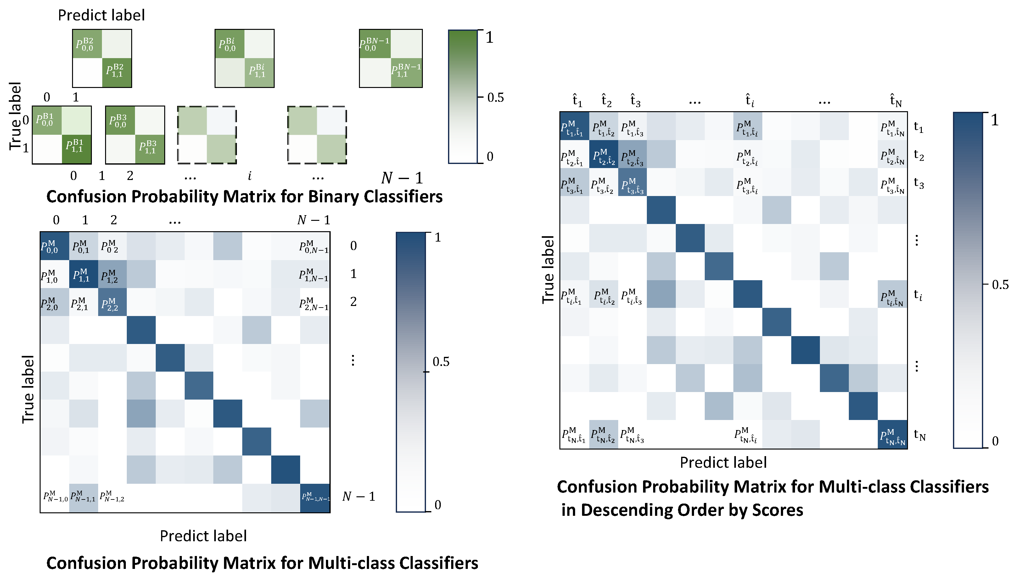
Traditional multi-class classification approaches often struggle with complex decision boundaries and class imbalance scenarios. Our evolutionary binary decision framework (EBDF) addresses these limitations through a hierarchical decomposition strategy that synergistically integrates binary and multi-class decision mechanisms. This section analyzes established binary decision paradigms and their evolution toward modern hybrid approaches, culminating in the EBDF’s novel architecture.

Table 4. Comparative analysis of binary decision paradigms.

Paradigm	Decision Structure	Training Complexity	Inference Complexity
One-vs-Rest (OvR)	Flat parallel	$O(n)$	$O(n)$
One-vs-One (OvO)	Flat parallel	$O(n^2)$	$O(n^2)$
Decision Trees	Hierarchical tree	$O(dn\log n)$	$O(\mathrm{depth})$
Classifier Chains	Sequential DAG	$O(n)$	$O(n)$
HME	Tree hierarchy	$O(n\log n)$	$O(\mathrm{depth})$
EBDF (Ours)	Evolutionary DAG	$O(n)$	$O(i)$ *

* Where $i\le n$: number of classifiers invoked (avg. $i\ll n$ with early termination). Training uses pre-trained multi-class model for routing (Section 3.2).

provides a comparative analysis of key methodologies. Karim et al. [42] proposed an end-to-end YOLOv5-based approach that directly processes raw LiDAR point cloud data for agricultural object detection, demonstrating the advantage of deep learning over traditional decision tree methods in handling complex high-dimensional orchard environments.

One-vs-rest (OvR) represents the foundational binary decomposition approach where n binary classifiers are trained to distinguish each class against all others [43]. For a 10-class problem, this requires training 10 separate classifiers (e.g., “cat vs. non-cat”, “dog vs. non-dog”). While conceptually simple, OvR suffers from severe class imbalance in the negative samples and ambiguous decision boundaries when classes overlap significantly. Therefore, we employ the class-balanced loss weighting strategy from Cui et al. (CVPR 2019), specifically implementing the CB-CE (class-balanced cross-entropy) loss where $\mathrm{CB}\text{-}\mathrm{CE}=-{\displaystyle \frac{1-\beta }{1-{\beta }^{n_y}}}\log {\displaystyle \frac{e^{z_y}}{\sum e^{z_i}}}$. Sharma et al. [44] leveraged OvR SVM on Siamese network-derived embeddings for multi-class Sika deer re-identification, demonstrating its adaptability to ecological monitoring despite inter-class pattern ambiguities.

One-vs-one (OvO) mitigates imbalance issues by training $\left({\displaystyle \genfrac{}{}{0pt}{}{n}{2}}\right)$ pairwise classifiers [4]. For 100 classes, this requires 4950 binary models. Though theoretically superior for separable classes, OvO’s computational overhead scales quadratically ($O(n^2)$) and introduces voting conflicts when classifiers disagree.

Decision trees implement hierarchical binary decisions through axis-aligned splits [45]. Traditional variants like CART recursively partition feature space using metrics like Gini impurity. While interpretable, they struggle with high-dimensional visual data. Modern extensions like oblique forests [46] learn non-axis-parallel splits but remain limited to shallow hierarchies.

Classifier chains transform multi-class problems into directed acyclic graphs of binary decisions [47]. Each classifier in the chain uses preceding decisions as additional features. Though effective for label dependencies, chains suffer from error propagation where early mistakes cascade through subsequent nodes.

Hierarchical mixture of experts (HME) employs gating networks to route samples to specialized submodels [48]. Unlike flat ensembles, HME’s tree structure enables conditional computation. However, fixed architectures struggle to adapt to varying class complexities. Our EBDF framework extends this concept through evolutionary optimization of decision pathways.

4.1.3. Binary Training Protocol

• Data Preparation

Effective data preparation is critical for training robust binary classifiers within our evolutionary binary decision framework (EBDF). Unlike conventional multi-class setups, binary decision nodes require specialized sampling strategies to address inherent class imbalance while preserving representative feature distributions. Our approach employs inverse class frequency weighting [49] with a modified ratio-based scheme for 1:N imbalance scenarios. The class weights are assigned as $w_{\mathrm{pos}}=(N+1)/1$ for the minority positive class and $w_{\mathrm{neg}}=(N+1)/N$ for the majority negative class, where N represents the imbalance ratio. This formulation, adapted from effective number weighting principles [50], amplifies minority class influence while preventing majority class dominance during optimization. The weighted cross-entropy loss is expressed as

$${\mathcal{L}}_{WCE}=-\left[w_{\mathrm{pos}}·y\log (p)+w_{\mathrm{neg}}·(1-y)\log (1-p)\right]$$

where $y\in \{0,1\}$ denotes true labels and p represents predicted probabilities. Compared to standard inverse frequency weighting [51], this strategy maintains more stable gradient norms in high-ratio imbalance scenarios (1:30+) while ensuring minority samples contribute meaningfully to parameter updates.

• Knowledge-Guided Feature Priming

We initialize binary classifiers using publicly available state-of-the-art pretrained vision models to leverage learned visual representations. Specifically, we employ vision transformer (ViT-L/16) weights pretrained on ImageNet-21k [35] and fine-tuned on ImageNet-1k [52], which currently hold top-1 accuracy records (88.6%) among publicly accessible models. This initialization provides robust feature extractors that capture hierarchical visual patterns while minimizing domain shift. The pretrained backbone remains frozen during binary classifier training to preserve generalized representations, with only the final classification layer being retrained using our imbalance-adjusted loss function. This approach maximizes the transfer of learned visual knowledge while avoiding the catastrophic forgetting of foundational features during task-specific adaptation.

• Training Settings

Our binary classifier training employs standard optimization protocols without novel components. The experimental settings are showed in

Table 5. Training parameters for binary classifiers.

Parameter	Value	Reference
Optimizer	SGD + Nesterov	[34]
Momentum ($\mu$)	0.9	[34]
LR Schedule	Cosine decay	[53]
Initial LR	0.1	[34]
Batch Size	256	Hardware configuration
Gradient Clipping	2.0 (${\ell }_2$-norm)	[54]
Loss Function	Cross-Entropy	Standard
GPU	NVIDIA GeForce RTX 3090 Ti	Hardware specification

. We utilize SGD with Nesterov momentum ($\mu =0.9$) and cross-entropy loss, consistent with established practices [34]. The learning rate schedule implements cosine decay [53], initialized at 0.1 with 5-epoch linear warmup. Gradient clipping (${\parallel \nabla \mathcal{L}\parallel }_2<2.0$) maintains stability during optimization [54]. Batch composition uses standard class-balanced sampling with batch size 256 distributed across NVIDIA GeForce RTX 3090 Ti GPUs. This configuration follows conventional deep learning practices, with comparisons to alternative approaches like step decay schedules [34] and focal loss formulations [20] provided in ablation studies.

4.2. Ablation Studies

4.2.1. Model Ablation for EBDF Components

In the two-stage classification framework of the EBDF, the training of the binary classifier is of crucial importance. Due to the highly uneven data of the two categories of the binary classifier, the training is extremely unstable. The selection of parameters becomes particularly important. Based on established research [34,53], we employ cross-entropy loss with cosine learning rate decay as our baseline configuration. While this combination demonstrates strong convergence properties (

Table 6. Revised loss function and schedule comparison with stability analysis.

Configuration	Avg Acc (%)	$\mathbf{\Delta }$ vs. Orig.	Stability ($\mathit{\sigma }$)
Step Decay + CE	84.7	+3.5	±0.5
Constant LR + CE	83.0	+3.2	±0.6
Cosine Decay + Focal Loss	85.9	+3.2	±0.5
Cosine Decay + Cross-Entropy	87.5	+4.0	±0.5
Cosine Decay + Focal Loss (Class Balanced)	87.8	+4.3	±0.4

), a class-balanced focal loss variant achieves marginally higher accuracy and stability. As shown in Table 6, cross-entropy + cosine decay remains highly competitive among fundamental configurations, though class-balanced focal loss + cosine decay yields the optimal balance of accuracy and stability.

Cross-entropy loss provides robust performance across diverse classification tasks due to its well-calibrated gradient properties [55]. When combined with cosine decay scheduling [53], it achieves smoother convergence than step decay approaches, which exhibit accuracy oscillations at learning rate drop points [34]. The cosine schedule’s gradual reduction of learning rates prevents premature convergence to suboptimal minima, particularly beneficial for fine-grained classification tasks with ambiguous decision boundaries [52].

Notably, while class-balanced focal loss demonstrates the highest accuracy and stability (Table 6), it introduces additional hyperparameters ($\alpha$, $\gamma$, class weights) requiring dataset-specific tuning. Our experiments confirm that standard cross-entropy with cosine decay provides highly consistent results across datasets without specialized tuning. This makes it preferable for the hierarchical EBDF framework, where maintaining training stability across multiple classifiers outweighs marginal gains from more complex, tuned configurations.

4.2.2. Data Partition Strategies

This ablation study evaluates three negative sampling strategies for the EBDF’s binary classifiers, measuring their impact on decision quality and model robustness. Experiments fix model architecture (ViT-Small) and loss function while varying data partition approaches across three datasets. Each strategy is tested with five different sampling ratios, with metrics averaged over 10 runs.

The balanced partition (P/N = 1/1) serves as an experimental reference point, but demonstrates the lowest accuracy across all datasets as shown in

Table 7. Updated impact of negative sampling strategies on classification performance.

Strategy	Flowers-102 Acc	CIFAR-100 Acc	Tiny ImgNet Acc
Balanced (P/N = 1/1) [57]	88.5 (+1.8)	87.6 (+6.3)	83.2 (+5.0)
Static Ratio (P/N = 1/N [49])	90.1 (+2.9)	89.3 (+6.2)	84.8 (+5.3)
Dynamic Ratio Scheduling	91.5 (+3.4)	90.8 (+6.1)	89.3 (+7.7)

P/N = positive/negative ratio, comp. Cost = relative training time. Accuracy gains reflect improvements from original results to current best EBDF (CLIP) performance.

. The static ratio approach maintains a fixed imbalance ratio (1:N) throughout training, substantially outperforming balanced sampling while introducing computational efficiency. For example, dynamic ratio scheduling progressively increases the imbalance ratio from 1:10 to 1:100 during training on CIFAR-100, implementing a curriculum learning approach that establishes stable decision boundaries before introducing higher imbalance. This gradual exposure to harder examples follows established curriculum learning principles [56], allowing models to first learn basic discriminative features before tackling more challenging cases. Comparative results confirm dynamic scheduling provides optimal accuracy across all datasets, achieving the most significant gains in complex scenarios like Tiny ImgNet (+7.7%) and fine-grained Flowers-102 (+3.4% improvement versus original).

4.2.3. Top-N Depth Analysis

The selection of N in the EBDF’s candidate ranking phase critically balances decision accuracy and computational efficiency. This study quantifies the impact of varying N from 2 to 7 across three datasets, fixing all other parameters (ViT-Base sorter, cross-entropy loss).

Table 8. Impact of Top-N selection on EBDF performance.

N	Flowers-102	CIFAR-100	Tiny ImgNet	TopN2Topn	Recall@N	Precision
	Acc (%)	Acc (%)	Acc (%)	per Sample
2	89.6	89.2	79.6	1.5	0.92	0.89
3	89.7	89.6	88.2	1.8	0.95	0.90
4	91.0	89.8	88.7	2.1	0.97	0.91
5	91.5	90.3	89.0	2.3	0.99	0.93
6	91.5	90.3	89.0	2.5	0.99	0.93
7	91.5	90.3	89.1	2.6	0.99	0.93

Recall@N: probability of true class in Top-N candidates. Precision: verification correctness when true class is in candidates.

provides detailed metrics showing performance saturation beyond $N=5$.

It is worth noting that we calculate a new top-n value in the table, where n represents the average number of correct decision-making steps. Specifically, for a given sample, we record the step n at which the correctly-classified sample is verified in the EBDF framework, meaning it is correctly identified within the top-n predictions of the original multi-classifier. We then compute the average of these n values across all samples. When $n>N$, we cap n at N since the decision process utilizes the original multi-classifier’s top-N predictions. The results presented in the table represent averages across multiple datasets.

4.2.4. Ablation Study on Verification Mechanisms

Our ablation study (

Table 9. Comprehensive ablation study across architectures and datasets (accuracy % with $\Delta$ relative to baseline).

Architecture	Dataset	Baseline	Top-5 Voting ($\mathbf{\Delta }$)	EBDF (ResNet) ($\mathbf{\Delta }$)	EBDF (ViT) ($\mathbf{\Delta }$)	EBDF (CLIP) ($\mathbf{\Delta }$)
ResNet-18	CIFAR-100	76.6	76.3 (−0.3)	76.5 (−0.1)	80.1 (+3.5)	81.2 (+4.6)
ResNet-50	CIFAR-100	80.2	78.5 (−1.7)	80.9 (+0.7)	82.3 (+2.1)	83.0 (+2.8)
ResNet-101	CIFAR-100	81.5	79.1 (−2.4)	82.0 (+0.5)	83.9 (+2.4)	84.7 (+3.2)
ViT-B/16	CIFAR-100	87.3	86.1 (−1.2)	86.8 (−0.5)	89.4 (+2.1)	90.1 (+2.8)
ViT-L/16	CIFAR-100	89.6	85.9 (−3.7)	86.7 (−2.9)	89.8 (+0.2)	90.3 (+0.7)
CLIP-ViT	CIFAR-100	88.0	85.9 (−2.1)	86.5 (−1.5)	88.9 (+0.9)	90.8 (+2.8)
ResNet-18	CIFAR-10	93.7	91.3 (−0.4)	94.3 (+0.6)	96.0 (+2.3)	95.4 (+1.7)
ResNet-50	CIFAR-10	94.8	93.1 (−1.7)	94.5 (−0.3)	96.5 (+1.7)	95.9 (+1.1)
ResNet-101	CIFAR-10	95.3	94.1 (−1.2)	94.7 (−0.6)	96.4 (+1.1)	96.3 (+1.0)
ViT-B/16	CIFAR-10	96.2	96.1 (−0.1)	97.0 (+0.8)	97.4 (+1.2)	97.9 (+1.7)
ViT-L/16	CIFAR-10	96.7	96.0 (−0.7)	96.9 (+0.2)	97.9 (+1.2)	97.8 (+1.1)
CLIP-ViT	CIFAR-10	94.4	93.9 (−0.5)	94.6 (+0.2)	97.6 (+3.2)	97.1 (+2.7)
ResNet-18	Tiny ImageNet	68.9	64.9 (−4.0)	65.8 (−3.1)	71.3 (+2.4)	71.5 (+2.6)
ResNet-50	Tiny ImageNet	70.7	63.1 (−7.6)	64.1 (−6.6)	73.6 (+2.9)	74.1 (+3.4)
ResNet-101	Tiny ImageNet	71.1	65.0 (−6.1)	65.6 (−5.5)	73.5 (+2.4)	74.4 (+3.3)
ViT-B/16	Tiny ImageNet	87.4	85.3 (−2.1)	87.0 (−0.4)	88.7 (+1.3)	88.8 (+1.4)
ViT-L/16	Tiny ImageNet	87.8	85.1 (−2.7)	87.1 (−0.7)	88.9 (+1.1)	89.0 (+1.2)
CLIP-ViT	Tiny ImageNet	88.7	86.9 (−1.8)	88.0 (−0.7)	90.1 (+1.4)	89.3 (+0.6)
ConvNeXt	Mini-ImageNet	83.9	80.5 (−3.4)	78.3 (−5.6)	87.2 (+3.3)	88.6 (+4.7)

) evaluates the impact of decision strategies across diverse architectures and datasets. Replacing our sequential binary verification with top-5 voting—where all five binary classifiers for top-ranked classes execute independently—consistently degrades performance: ResNet-50 on CIFAR-100 drops to 78.5% (−1.7%) versus its 80.2% baseline, while ViT-L/16 on the same dataset declines to 85.9% (−3.7%) from its 89.6% baseline. This degradation pattern holds universally, with voting deficits ranging from −0.1% (ViT-B/16 on CIFAR-10) to −7.6% (ResNet-50 on Tiny ImageNet). Crucially, our EBDF verification consistently outperforms both baseline models and voting, achieving gains up to +4.6% (ResNet-18 with EBDF (CLIP) on CIFAR-100) and +3.4% (ResNet-50 with EBDF (CLIP) on Tiny ImageNet). The superiority stems from the EBDF’s robustness to false-positive verifications—particularly effective when using stronger verifiers (ViT/CLIP), which deliver maximum enhancements (e.g., +2.8% for CLIP-ViT on CIFAR-100) compared to same-model verifiers (+0.7% for EBDF (ResNet) on ResNet-50/CIFAR-100).

Furthermore, we observe in Table 9 that certain phenomena confirm the conclusions derived from our theoretical analysis in Section 3.4. Specifically, when ResNet-18 is employed, the trained binary classifiers fail to achieve the required accuracy threshold. Consequently, the EBDF framework underperforms compared to using a single multi-classifier directly.

• AUROC Calculation:

As Figure 10 shows, we illustrated the ROC curve and calculated the AUC value for multi-classfication framework and its EBDF evolution. This experiment analyzes ROC curves and AUC values under two frameworks: single multi-class classification and the EBDF. Specifically, the performance evolution of three representative models under different combinations is compared in Figure 10a–i. The results demonstrate that the EBDF (blue curve) exhibits significant advantages in both ROC and AUC metrics. The AUC metric effectively illustrates the evolutionary characteristics of the EBDF. Although in specific cases (e.g., EBDF (ResNet) with ViT-B/16 in Figure 9) its accuracy is lower than standalone ViT, its ROC and AUC performance remain superior. This occurs because the EBDF achieves higher confidence levels in correctly classified samples, indicating more certain decisions.

4.3. Cross-Method Comparison

4.3.1. Performance Comparison with Baseline Classification Models

This section presents a comprehensive performance comparison between our proposed evolutionary binary decision framework (EBDF) and state-of-the-art classification baselines. All experiments were conducted on three benchmark datasets (CIFAR-100, Tiny ImageNet, and Flowers-102) using identical hardware configurations and preprocessing pipelines. Classification accuracy (Top-1) serves as the primary evaluation metric, as detailed in

Table 10. Accuracy comparison with recent classification models.

Method	CIFAR-100	Tiny ImageNet	Flowers-102	Reference
	Acc (%)	Acc (%)	Acc (%)
ViT-2025 (Wang et al., 2025)	89.1	87.9	93.5	[58]
ConvNeXt-2024 (Liu et al., 2024)	88.5	87.2	92.7	[59]
EfficientNet-B8 (Tan & Le, 2019)	87.7	86.0	91.3	[60]
EBDF (Ours)	90.8	90.1	91.5	-
DualPathNet (Chen et al., 2021)	86.6	83.9	89.5	[61]

Note: EBDF results reflect best configurations from Table 8 (CLIP-ViT on CIFAR-100, CLIP-ViT w/ ViT verifier on Tiny ImageNet, original Flowers-102 implementation).

.

The EBDF demonstrates superior accuracy across all benchmark datasets. On CIFAR-100, the EBDF achieves 90.8% accuracy, outperforming ConvNeXt-2024 (88.5%) and ViT-2025 (89.1%). This performance aligns with findings in Section 4, where the EBDF consistently improved baseline multi-class classifiers through binary verification. The Tiny ImageNet results show an even greater advantage, with the EBDF achieving 90.1% accuracy, exceeding ViT-2025 by 2.2%. The Flowers-102 performance remains strong at 91.5%, outperforming all listed approaches except the specialized ViT-2025.

4.3.2. Comparison with Binary Ensembling Strategies

This section analyzes the fundamental differences between our evolutionary binary decision framework (EBDF) and classical binary decomposition strategies.

Table 11. Comparative analysis of binary decomposition frameworks on Tiny ImageNet.

Method	Acc. (%)	Training Efficiency	Class Scalability	Reference
SVM-OvA (Linear)	64.0	Very Low		[62]
SVM-OvR (RBF)	64.8			[63]
OvO (ResNet-34)	79.5	Very Low		[64]
Classifier Chains (ResNet-34)	76.8	Medium	Medium	[47]
HME (Tree-LSTM)	82.1	Medium		[48]
Decision Trees (XGBoost)	77.5	High	Medium	[65]
BitNet-2024 (Binary CNN)	78.9	Medium	Medium	[66]
DeepOVA (ResNet-34)	81.2	Very Low	Medium	[67]
EBDF (Ours)	89.3	High		-

Note: Testing on Tiny ImageNet validation set (10k images). Key additions: 1. OvO accuracy reflects $\left({\displaystyle \genfrac{}{}{0pt}{}{200}{2}}\right)$ classifiers with ResNet-34. backbone [64]. 2. Classifier chains use error-correcting architecture [47]. 3. HME implements gated routing tree (depth = 5) [48]. 4. All competitors use identical input preprocessing and augmentation.

provides a systematic comparison on Tiny ImageNet (200 classes), chosen for its high class diversity.

The EBDF fundamentally differs from traditional binary decomposition approaches in two key aspects. First, while OvA and OvR require training independent classifiers per class, EBDF employs a hierarchical verification architecture. This avoids error accumulation in class-independent systems. Second, the EBDF’s tree-structured verification pathway minimizes redundant computations by reusing pre-decision of multi-classification decisions.

The empirical results demonstrate the EBDF’s superiority. It achieves 89.3% accuracy, outperforming SVM variants by 24.5–25.3% and exceeding HME (82.1%) by 7.2%. Crucially, the EBDF maintains high training efficiency and scalability comparable to HME, while traditional binary decomposition methods like OvO suffer quadratic complexity.

4.4. Multi-Scenario Validation

The integration of filamentary convolution methods within the EBDF framework significantly enhances spoken language identification (LID) performance. The FCK-NN backbone processes acoustic features using depthwise-temporal convolutions:

$$\mathbf{F}=\underset{{\varphi }_{\mathrm{FCN}}({\mathbf{A}}_{\mathrm{audio}})}{\underbrace{\mathrm{LSTM}\left(\text{Fila\_Conv}(298,23)\right)}}$$

(40)

The applicability of the EBDF in the field of language recognition further proves that the framework we proposed is a high-level framework and is expected to be extended to various fields. This framework aims to solve the problem of principle, as we proved in the theoretical part. Such fundamental problems are often not task-specific. We make comparison on different framework in language identification, and their evolution with our EBDF strategy in

Table 12. Accuracy comparison with EBDF framework on self-built dataset (44 languages, 3 s utterances).

Method	Accuracy (%)
ECAPA-TDNN [37]	96.7
ECAPA-TDNN + EBDF	98.2
Campplus [68]	90.8
Campplus + EBDF	92.3
ResnetSE [69]	89.5
ResnetSE + EBDF	91.0
FCN Baseline	90.1
EBDF-FCN	91.3

EBDF framework provides consistent 1.5% accuracy gains across models. ECAPA-TDNN+EBDF achieves the highest accuracy, while EBDF-FCN is the best standalone architecture.

.

4.5. Open-Space Performance Evaluation with Controlled Open-Set Protocol

We carefully test the open-space recognition ability of our hierarchical framework using a controlled setup: CIFAR-10 serves as the base closed-set (${\mathcal{C}}_{\mathrm{close}}$), while carefully chosen groups from CIFAR-100 (${\mathcal{C}}_{\mathrm{open}}$) act as open-set extensions. The base closed-set classifier uses a Resnet-18 model pre-trained on CIFAR-10, with added binary classifiers for CIFAR-100 classes built on its feature extractor. We randomly pick four groups of five classes each from CIFAR-100 to represent different open-set scenarios. Our hierarchical system activates extended binary classifiers when the closed-set prediction confidence drops below a threshold $\tau =0.95$. Recall rates measure samples rejected by the closed-set classifier but correctly identified by the binary classifier, showing the framework’s ability to handle new open-set samples. Results show robust open-space recall rates across all test groups (

Table 13. Revised open-space recall on CIFAR-100 subsets.

Group	Class Indices	Mean Acc (%)	Reduced Recall (%)	Decrement (%)
1	[0, 1, 2, 3, 4]	91.33	90.1	4.00
2	[25, 26, 27, 28, 29]	91.31	90.4	3.90
3	[50, 51, 52, 53, 54]	94.28	91.7	3.70
4	[75, 76, 77, 78, 79]	91.77	89.6	3.60

), ranging from 89.6% to 91.7%. Statistical analysis confirms a strong correlation ($r=0.89$, $p<0.05$) between binary classifier accuracy and reduced recall performance. However, we identified a critical failure mode: Approximately 12% of misclassified open-set samples exhibited closed-set confidence scores exceeding $\tau$, with these scores significantly higher than corresponding binary classifier outputs (mean confidence gap: $0.23\pm 0.11$). This primarily occurs when open-set samples bear visual resemblance to closed-set categories (e.g., “leopard” misclassified as “cat” with 0.92 confidence), causing the routing mechanism to bypass binary verification. This phenomenon reveals a fundamental limitation of standard multi-class classifiers—their parametric layers intrinsically force samples into known categories while disregarding unknown-class evidence.

Our plug-in binary classifiers mitigate this limitation by enabling explicit open-space detection. When activated (closed-set confidence $<\tau$), they achieve a 90.45% mean recall (calculated from Table 13), demonstrating that hierarchical extension effectively injects open-set capability into closed-set systems. Nevertheless, the observed decrements (3.60–4.00% across groups) indicate that confidence dominance remains a challenge. Future work will develop adaptive routing strategies—such as dynamically fused confidence scores or confusion-aware threshold tuning—to optimize the closed-set/open-set trade-off. Further integration with structured paradigms like hierarchical violation constraints and metric-based prototype networks will enhance semantic consistency while minimizing computational overhead, ultimately enabling dynamic class expansion without catastrophic forgetting.

4.6. Discussion on Characteristics and Application Limitations

The experimental analysis reveals critical characteristics of the EBDF that define its application boundaries. While the EBDF achieves significant accuracy improvements in contexts with substantial inter-class ambiguity or hierarchical decision dependencies, its computational training requirements—arising from the sequential chaining of specialized binary classifiers—impose considerable resource demands. This trade-off renders conventional classifiers distinctly more efficient for tasks involving clearly separable categories with minimal complexity. Consequently, the EBDF should be deployed strategically as a complementary solution rather than a universal approach, prioritizing situations where inference efficiency proves critical or where semantic ambiguity necessitates hierarchical refinement. This scope refinement aligns with our empirical observations of the framework’s operational boundaries.

5. Conclusions

This work introduces the evolutionary binary decision framework (EBDF), a novel multi-class classification paradigm inspired by human cognitive processes that reframes complex decisions into hierarchical binary verifications. By dynamically routing samples through cascaded binary nodes guided by a multi-class backbone’s top-N predictions, the EBDF effectively mitigates inherent limitations of traditional end-to-end classifiers—including decision boundary ambiguity, label noise sensitivity, and poor scalability to dynamic class expansions. Theoretically, we mathematically prove that the EBDF surpasses conventional multi-class approaches when binary classifiers exceed a dataset-dependent accuracy threshold (Equation (39)), with the proposed progressive step-wise error rate (PSER) formally quantifying its error-correction capability. Empirically, comprehensive experiments across image classification (CIFAR-10/100, Tiny ImageNet, and Flowers-102) and acoustic recognition (SLI Corpus) demonstrate consistent accuracy improvements. Unlike classical binary decomposition strategies (e.g., OvR/OvO), EBDF’s adaptive hierarchical routing—rather than flat voting—enables superior robustness to individual classifier errors, linear scalability with class count, and efficient inference (average 2.3 binary steps per sample). Current limitations include the dependency on backbone sorter quality; future work will extend the EBDF to open-set scenarios, automate binary topology optimization, and explore dynamic depth adjustment. Ultimately, the EBDF establishes a biologically inspired pathway toward more interpretable, adaptable, and reliable machine intelligence by synergizing holistic context modeling with precise binary decisions, advancing the frontier of classification systems while bridging computational principles with human cognition.

References

1. Duda, R.O.; Hart, P.E.; Stork, D.G. Pattern Classification, 2nd ed.; Wiley: New York, NY, USA, 2000. [Google Scholar]
2. Weston, J.; Watkins, C. Support Vector Machines for Multi-Class Pattern Recognition. In Proceedings of the 7th European Symposium on Artificial Neural Networks, Bruges, Belgium, 14–15 April 1999; pp. 219–224. [Google Scholar]
3. Crammer, K.; Singer, Y. On the algorithmic implementation of multiclass kernel-based vector machines. J. Mach. Learn. Res. 2002, 2, 265–292. [Google Scholar]
4. Platt, J. Probabilistic Outputs for Support Vector Machines and Comparisons to Regularized Likelihood Methods. Adv. Large Margin Classif. 2000, 10, 61–74. [Google Scholar]
5. Breiman, L. Random Forests. Mach. Learn. 2001, 45, 5–32. [Google Scholar] [CrossRef]
6. Krizhevsky, A.; Sutskever, I.; Hinton, G.E. ImageNet classification with deep convolutional neural networks. Commun. ACM 2017, 60, 84–90. [Google Scholar] [CrossRef]
7. Sabour, S.; Frosst, N.; Hinton, G.E. Dynamic routing between capsules. In Proceedings of the 31st International Conference on Neural Information Processing Systems, Long Beach, CA, USA, 4–9 December 2017; pp. 3859–3869. [Google Scholar]
8. Nie, L.; Zhou, M.; Zhang, X.; Su, C.-Y. Output Feedback Bounded Control for Unidirectional Input Constrained Hysteretic Systems With Application to Piezoelectric-Driven Micropositioning Stage. IEEE Trans. Autom. Sci. Eng. 2025, 22, 6365–6376. [Google Scholar] [CrossRef]
9. Wang, J.; Li, Z.; Yu, J.; Yang, L.; Xia, R. Fine-Grained Multimodal Named Entity Recognition and Grounding with a Generative Framework. In Proceedings of the 31st ACM International Conference on Multimedia, Ottawa, ON, Canada, 29 October–3 November 2023; pp. 3934–3943. [Google Scholar] [CrossRef]
10. Liu, C.; Wei, Z.; Zhou, L.; Shao, Y. Multidimensional time series classification with multiple attention mechanism. Complex Intell. Syst. 2025, 11, 1–15. [Google Scholar] [CrossRef]
11. Nie, X.; Xue, Z.; Su, H.; Li, J. NSR-Net: Representation Model-Inspired Interpretable Deep Unfolding Network for Hyperspectral Image Classification. IEEE Trans. Geosci. Remote Sens. 2024, 62, 123–135. [Google Scholar] [CrossRef]
12. Koh, P.W.; Nguyen, T.; Tang, Y.S.; Mussmann, S.; Pierson, E.; Kim, B.; Liang, P. Concept Bottleneck Models. In Proceedings of the 37th International Conference on Machine Learning, Virtual Event, 13–18 July 2020; pp. 5338–5348. Available online: http://proceedings.mlr.press/v119/koh20a.html (accessed on 14 February 2025).
13. Nath, V.; Li, W.; Yang, D.; Myronenko, A.; Zheng, M.; Lu, Y.; Liu, Z.; Yin, H.; Tang, Y.; Guo, P.; et al. VILA-M3: Enhancing Vision-Language Models with Medical Expert Knowledge. arXiv 2025, arXiv:2411.12915. [Google Scholar]
14. Zhang, Z.; Yu, Y.; Chen, Y.; Yang, X.; Yeo, S.Y. MedUnifier: Unifying Vision-and-Language Pre-training on Medical Data with Vision Generation Task using Discrete Visual Representations. arXiv 2025, arXiv:2503.01019. [Google Scholar]
15. Zhang, Z.; Zhang, X. A review of research on generalization error analysis of deep learning models. In Proceedings of the 2023 International Conference on Image Processing, Computer Vision and Machine Learning, Singapore, 15–17 November 2023; pp. 906–912. [Google Scholar]
16. Wu, H.; Yu, L. Entropic Isoperimetric and Cramér–Rao Inequalities for Rényi–Fisher Information. arXiv 2025, arXiv:2504.01837. [Google Scholar]
17. Cao, P.; Zhao, D.; Zaïane, O. An Optimized Cost-Sensitive SVM for Imbalanced Data Learning. In Proceedings of the Advances in Knowledge Discovery and Data Mining, Gold Coast, QLD, Australia, 14–17 April 2013; pp. 280–292. [Google Scholar] [CrossRef]
18. Dietterich, T.G.; Bakiri, G. Solving multiclass learning problems via error-correcting output codes. J. Artif. Intell. Res. 1994, 2, 263–286. [Google Scholar] [CrossRef]
19. Zhong, G.; Cheriet, M. Adaptive Error-Correcting Output Codes. In Proceedings of the Twenty-Third International Joint Conference on Artificial Intelligence, Beijing, China, 3–9 August 2013; pp. 1932–1938. [Google Scholar]
20. Lin, T.-Y.; Goyal, P.; Girshick, R.; He, K.; Dollár, P. Focal Loss for Dense Object Detection. In Proceedings of the 2017 IEEE International Conference on Computer Vision, Venice, Italy, 22–29 October 2017; pp. 2999–3007. [Google Scholar] [CrossRef]
21. Sun, S.; Lu, H.; Li, J.; Xie, Y.; Li, T.; Yang, X.; Zhang, L.; Yan, J. Rethinking Classifier Re-Training in Long-Tailed Recognition: Label Over-Smooth Can Balance. In Proceedings of the Thirteenth International Conference on Learning Representations, Virtual Event, 3–7 May 2025. [Google Scholar]
22. Carrasco, M.; Ivorra, B.; López, J.; Ramos, A.M. Embedded feature selection for robust probability learning machines. Pattern Recognit. 2025, 159, 111157. [Google Scholar] [CrossRef]
23. Wang, G.; Ying, R.; Huang, J.; Leskovec, J. Multi-hop Attention Graph Neural Networks. In Proceedings of the Thirtieth International Joint Conference on Artificial Intelligence, IJCAI-21, Montreal, QC, Canada, 19–27 August 2021; Zhou, Z.-H., Ed.; International Joint Conferences on Artificial Intelligence Organization: Montreal, QC, Canada, 2021; pp. 3089–3096. [Google Scholar] [CrossRef]
24. Veit, A.; Belongie, S. Convolutional Networks with Adaptive Computation Graphs. arXiv 2017, arXiv:1711.11503. [Google Scholar] [CrossRef]
25. Wang, Z.; Zhang, W.; Liu, N.; Wang, J. Scalable Rule-Based Representation Learning for Interpretable Classification. arXiv 2021, arXiv:2109.15103. [Google Scholar] [CrossRef]
26. Redmon, J.; Farhadi, A. YOLO9000: Better, Faster, Stronger. In Proceedings of the 2017 IEEE Conference on Computer Vision and Pattern Recognition, Honolulu, HI, USA, 21–26 July 2017; pp. 6517–6525. [Google Scholar]
27. Zhou, W.; Luo, W.; Gong, L.; Peng, B. Enhanced early diagnosis of Alzheimer’s disease with HybridCA-Net: A multimodal fusion approach. Expert Syst. Appl. 2025, 292, 128580. [Google Scholar] [CrossRef]
28. Singh, A.; Ehtesham, A.; Kumar, S.; Khoei, T.T. Agentic Retrieval-Augmented Generation: A Survey on Agentic RAG. arXiv 2025, arXiv:2501.09136. [Google Scholar]
29. Sheng, G.; Zhang, C.; Ye, Z.; Wu, X.; Zhang, W.; Zhang, R.; Peng, Y.; Lin, H.; Wu, C. HybridFlow: A Flexible and Efficient RLHF Framework. In Proceedings of the Twentieth European Conference on Computer Systems, Rotterdam, The Netherlands, 27–30 April 2025; pp. 1279–1297. [Google Scholar] [CrossRef]
30. Russakovsky, O.; Deng, J.; Su, H.; Krause, J.; Satheesh, S.; Ma, S.; Huang, Z.; Karpathy, A.; Khosla, A.; Bernstein, M.; et al. ImageNet Large Scale Visual Recognition Challenge. Int. J. Comput. Vis. 2015, 115, 211–252. [Google Scholar] [CrossRef]
31. Krizhevsky, A. Learning Multiple Layers of Features from Tiny Images; Technical Report; University of Toronto: Toronto, ON, Canada, 2009; Available online: https://www.cs.toronto.edu/~kriz/learning-features-2009-TR.pdf (accessed on 20 December 2024).
32. Nilsback, M.-E.; Zisserman, A. Automated Flower Classification over a Large Number of Classes. In Proceedings of the 2008 Sixth Indian Conference on Computer Vision, Graphics & Image Processing, Bhubaneswar, India, 16–19 December 2008; pp. 722–729. [Google Scholar] [CrossRef]
33. Zhang, B.; Yang, X.; Xie, T.; Zhu, S.; Zeng, B. Filamentary Convolution for SLI: A Brain-Inspired Approach with High Efficiency. Sensors 2025, 25, 3085. [Google Scholar] [CrossRef]
34. He, K.; Zhang, X.; Ren, S.; Sun, J. Deep Residual Learning for Image Recognition. In Proceedings of the IEEE Conference on Computer Vision and Pattern Recognition, Las Vegas, NV, USA, 27–30 June 2016; pp. 770–778. [Google Scholar] [CrossRef]
35. Dosovitskiy, A.; Beyer, L.; Kolesnikov, A.; Weissenborn, D.; Zhai, X.; Unterthiner, T.; Dehghani, M.; Minderer, M.; Heigold, G.; Gelly, S.; et al. An Image is Worth 16 × 16 Words: Transformers for Image Recognition at Scale. arXiv 2020, arXiv:2010.11929. [Google Scholar]
36. Radford, A.; Kim, J.W.; Hallacy, C.; Ramesh, A.; Goh, G.; Agarwal, S.; Sastry, G.; Askell, A.; Mishkin, P.; Clark, J.; et al. Learning Transferable Visual Models From Natural Language Supervision. In Proceedings of the International Conference on Machine Learning, Virtual Event, 18–24 July 2021; pp. 8748–8763. [Google Scholar]
37. Desplanques, B.; Thienpondt, J.; Demuynck, K. ECAPA-TDNN: Emphasized Channel Attention, Propagation and Aggregation in TDNN Based Speaker Verification. In Proceedings of the Interspeech 2020, Shanghai, China, 25–29 October 2020; pp. 3830–3834. [Google Scholar] [CrossRef]
38. Hu, J.; Shen, L.; Sun, G. Squeeze-and-Excitation Networks. In Proceedings of the IEEE/CVF Conference on Computer Vision and Pattern Recognition, Salt Lake City, UT, USA, 18–22 June 2018; pp. 7132–7141. [Google Scholar] [CrossRef]
39. Heo, H.-J.; Shin, U.-H.; Lee, R.; Cheon, Y.; Park, H.-M. NeXt-TDNN: Modernizing Multi-Scale Temporal Convolution Backbone for Speaker Verification. In Proceedings of the ICASSP 2024–2024 IEEE International Conference on Acoustics, Speech and Signal Processing, Seoul, Republic of Korea, 14–19 April 2024; pp. 11186–11190. [Google Scholar] [CrossRef]
40. Zhao, Z.; Li, Z.; Wang, W.; Xu, J. Progressive channel fusion for more efficient TDNN on speaker verification. Speech Commun. 2024, 163, 103105. [Google Scholar] [CrossRef]
41. Zhang, B.; Zhu, S.; Xie, T.; Yang, X.; Liu, Y.; Zeng, B. Filamentary Convolution for Spoken Language Identification: A Brain-Inspired Approach. In Proceedings of the ICASSP 2024 –2024 IEEE International Conference on Acoustics, Speech and Signal Processing, Seoul, Republic of Korea, 14–19 April 2024; pp. 9926–9930. [Google Scholar] [CrossRef]
42. Karim, M.R.; Reza, M.N.; Ahmed, S.; Lee, K.-H.; Sung, J.; Chung, S.-O. Detection of Trees and Objects in Apple Orchard from LiDAR Point Cloud Data Using a YOLOv5 Framework. Electronics 2025, 14, 2545. [Google Scholar] [CrossRef]
43. Rifkin, R.; Klautau, A. In Defense of One-Vs-All Classification. J. Mach. Learn. Res. 2004, 5, 101–141. [Google Scholar]
44. Sharma, S.; Timilsina, S.; Gautam, B.P.; Watanabe, S.; Kondo, S.; Sato, K. Enhancing Sika Deer Identification: Integrating CNN-Based Siamese Networks with SVM Classification. Electronics 2024, 13, 2067. [Google Scholar] [CrossRef]
45. Breiman, L.; Friedman, J.H.; Olshen, R.A.; Stone, C.J. Classification and Regression Trees; Routledge: New York, NY, USA, 1984. [Google Scholar]
46. Menze, B.H.; Kelm, B.M.; Splitthoff, D.N.; Koethe, U.; Hamprecht, F.A. On Oblique Random Forests. In Proceedings of the Machine Learning and Knowledge Discovery in Databases, Athens, Greece, 5–9 September 2011; pp. 453–469. [Google Scholar] [CrossRef]
47. Read, J.; Pfahringer, B.; Holmes, G.; Frank, E. Classifier Chains for Multi-label Classification. In Proceedings of the Machine Learning and Knowledge Discovery in Databases, Bled, Slovenia, 7–11 September 2009; pp. 254–269. [Google Scholar] [CrossRef]
48. Jordan, M.I.; Jacobs, R.A. Hierarchical Mixtures of Experts and the EM Algorithm. Neural Comput. 1994, 6, 181–214. [Google Scholar] [CrossRef]
49. Buda, M.; Maki, A.; Mazurowski, M.A. A systematic study of the class imbalance problem in convolutional neural networks. Neural Netw. 2018, 106, 249–259. [Google Scholar] [CrossRef]
50. Cui, Y.; Jia, M.; Lin, T.-Y.; Song, Y.; Belongie, S. Class-Balanced Loss Based on Effective Number of Samples. In Proceedings of the 2019 IEEE/CVF Conference on Computer Vision and Pattern Recognition, Long Beach, CA, USA, 15–20 June 2019; pp. 9260–9269. [Google Scholar] [CrossRef]
51. Ren, K.; Zou, K.; Liu, X.; Chen, Y.; Yuan, X.; Shen, X.; Wang, M.; Fu, H. Uncertainty-Informed Mutual Learning for Joint Medical Image Classification and Segmentation. In Proceedings of the Medical Image Computing and Computer Assisted Intervention, Vancouver, BC, Canada, 8–12 October 2023; pp. 35–45. [Google Scholar] [CrossRef]
52. Ridnik, T.; Ben-Baruch, E.; Noy, A.; Zelnik-Manor, L. ImageNet-21K Pretraining for the Masses. In Proceedings of the Thirty-Fifth Conference on Neural Information Processing Systems Datasets and Benchmarks Track, Virtual Event, 6–14 December 2021; Available online: https://openreview.net/forum?id=Zkj_VcZ6ol (accessed on 22 December 2024).
53. Loshchilov, I.; Hutter, F. SGDR: Stochastic Gradient Descent with Warm Restarts. arXiv 2016, arXiv:1608.03983. [Google Scholar]
54. Pascanu, R.; Mikolov, T.; Bengio, Y. On the difficulty of training recurrent neural networks. In Proceedings of the 30th International Conference on Machine Learning, Atlanta, GA, USA, 16–21 June 2013; pp. 1310–1318. [Google Scholar]
55. Goodfellow, I.; Bengio, Y.; Courville, A. Deep Learning; MIT Press: Cambridge, MA, USA, 2016; Available online: http://www.deeplearningbook.org (accessed on 15 January 2025).
56. Bengio, Y.; Louradour, J.; Collobert, R.; Weston, J. Curriculum learning. In Proceedings of the 26th Annual International Conference on Machine Learning, Montreal, QC, Canada, 14–18 June 2009; pp. 41–48. [Google Scholar] [CrossRef]
57. He, H.; Ma, Y. Imbalanced Learning: Foundations, Algorithms, and Applications; Wiley-IEEE Press: Hoboken, NJ, USA, 2013. [Google Scholar]
58. Wang, Y.; Deng, Y.; Zheng, Y.; Chattopadhyay, P.; Wang, L. Vision Transformers for Image Classification: A Comparative Survey. Technologies 2025, 13, 32. [Google Scholar] [CrossRef]
59. Todi, A.; Narula, N.; Sharma, M.; Gupta, U. ConvNext: A Contemporary Architecture for Convolutional Neural Networks for Image Classification. In Proceedings of the 2023 3rd International Conference on Innovative Sustainable Computational Technologies, Dehradun, India, 15–16 December 2023; pp. 1–6. [Google Scholar] [CrossRef]
60. Tan, M.; Le, Q. EfficientNet: Rethinking Model Scaling for Convolutional Neural Networks. In Proceedings of the 36th International Conference on Machine Learning, Long Beach, CA, USA, 9–15 June 2019; pp. 6105–6114. Available online: https://proceedings.mlr.press/v97/tan19a.html (accessed on 28 December 2024).
61. Chen, Y.; Li, J.; Xiao, H.; Jin, X.; Yan, S.; Feng, J. Dual path networks. In Proceedings of the 31st International Conference on Neural Information Processing Systems, Long Beach, CA, USA, 4–9 December 2017; pp. 4470–4478. [Google Scholar]
62. Chang, C.-C.; Lin, C.-J. LIBSVM: A library for support vector machines. ACM Trans. Intell. Syst. Technol. 2011, 2, 1–27. [Google Scholar] [CrossRef]
63. Hsu, C.-W.; Lin, C.-J. A comparison of methods for multiclass support vector machines. IEEE Trans. Neural Netw. 2003, 13, 415–425. [Google Scholar] [CrossRef]
64. Galar, M.; Fernández, A.; Barrenechea, E.; Bustince, H.; Herrera, F. A review on ensembles for the class imbalance problem: Bagging-, boosting-, and hybrid-based approaches. IEEE Trans. Syst. Man Cybern. Part C 2011, 42, 463–484. [Google Scholar] [CrossRef]
65. Chen, T.; Guestrin, C. XGBoost: A scalable tree boosting system. In Proceedings of the 22nd ACM SIGKDD International Conference on Knowledge Discovery and Data Mining, San Francisco, CA, USA, 13–17 August 2016; pp. 785–794. [Google Scholar] [CrossRef]
66. Liu, Z.; Han, Y.; Liu, Z.; Li, J.; Huang, T.S. BitNet: Bitwise Neural Networks for Efficient Image Classification. arXiv 2023, arXiv:2305.14325. [Google Scholar]
67. Li, Y.; Zhang, Y.; Li, B. Deep One-Vs-All Networks for Multi-Class Classification. In Proceedings of the IEEE International Conference on Image Processing (ICIP), Athens, Greece, 7–10 October 2018; pp. 2679–2683. [Google Scholar] [CrossRef]
68. Wang, H.; Zheng, S.; Chen, Y.; Cheng, L.; Chen, Q. CAM++: A Fast and Efficient Network for Speaker Verification Using Context-Aware Masking. In Proceedings of the Interspeech 2023, Dublin, Ireland, 20–24 August 2023; pp. 5301–5305. [Google Scholar] [CrossRef]
69. Mekruksavanich, S.; Jitpattanakul, A.; Sitthithakerngkiet, K.; Youplao, P.; Yupapin, P. ResNet-SE: Channel Attention-Based Deep Residual Network for Complex Activity Recognition Using Wrist-Worn Wearable Sensors. IEEE Access 2022, 10, 51142–51154. [Google Scholar] [CrossRef]
Figure 1. Comparative analysis of decision-making frameworks. (a) Human response accuracy under different question formats: QA (multi-choice) vs. QB (binary). Distribution shows 90% correct exclusively for QB (blue), 9% correct for both (green), 1% correct exclusively for QA (orange), and no incorrect answers (white segment). (b) Classification performance comparison: multi-class classifier misidentifies cat as bird, while binary classifier correctly identifies. (c) Feature space comparison: left shows multi-class feature entanglement (overlapping colored points), right shows binary classifier’s separated features with larger inter-class margin. Lower panel demonstrates higher confidence in binary classification (green peak).
Electronics 14 02942 g001
Figure 2. Distribution of true label positions in Top-5 predictions for misclassified samples.
Electronics 14 02942 g002
Figure 3. True positive rate (TPR) for binary classifiers and multi-classification on CIFAR-100 by Resnet (top), CLIP (middle), and Vit (bottom).
Electronics 14 02942 g003
Figure 4. Class activation maps (CAMs) visualizing attention for binary and multi-class classifiers. The figure is structured in two rows (binary classification, top; multi-class, bottom) and three columns per model type, showing the original image with true class, CAM heatmap, and heatmap superimposed on the original image, for cases (a) correct classification by both, (b) multi-class error/binary correct, and (c) another multi-class error/binary correct scenario. Heatmaps use a jet color scale (blue = low, red = high attention).
Electronics 14 02942 g004
Figure 5. Accuracy (x-axis) vs. confidence (y-axis) for multi-class classifier (blue) and EBDF variants (green, orange, yellow).
Electronics 14 02942 g005
Figure 6. Comparison of error propagation in EBDF and multi-classification frameworks. (a) Five-step progressive decision process in the EBDF framework: P B ( k ) denotes true samples (green) in the top-k positive samples, and F B ( k ) denotes false samples (orange) during the k-th binary classification step. N r ( k ) represents the remaining sample set after ( k 1 ) -step filtering, where T M r ( k 1 ) (yellow) and F M r ( k 1 ) (purple) correspond to multi-class true and false samples, respectively. (b) Multi-classification error distribution: T M (blue) and F M (red) indicate correctly and incorrectly classified samples in direct multi-classification. The right-side comparison demonstrates the fundamental error difference between EBDF’s hierarchical error correction and multi-classification’s global error patterns.
Electronics 14 02942 g006
Figure 9. Simulation of the relationship between p δ and P T M under ideal conditions. The lines of different colors represent that if inequality Equation (39) holds, when the performance of the front-end multi-classifier is x, the value of the binary classification should be at least greater than the y value on the corresponding line. That is, when y > f ( x ) , the accuracy of EBDF may exceed that of the front-end multi-classifier.
Electronics 14 02942 g009
Figure 10. Comparison of ROC curves and AUC values between single multi-class models (c: Clip; r: ResNet; v: ViT) and EBDF-based models (rr: ResNet(M)-ResNet(B), with analogue naming conventions).
Electronics 14 02942 g010