Transmission Opportunity and Throughput Prediction for WLAN Access Points via Multi-Dimensional Feature Modeling

Abstract

With the rapid development of wireless communication, Wireless Local Area Networks (WLANs) are widely deployed in high-density environments. Ensuring fast handovers and optimal AP selection during device roaming is critical for maintaining network throughput and user experience. However, frequent mobility, high access density, and dynamic channel fluctuations complicate throughput prediction. To address this, we propose a method combining the Snow-Melting Optimizer (SMO) with decision tree regression models to optimize feature selection and model transmission opportunities (TXOP) and AP throughput. Experimental results show that the Extreme Gradient Boosting (XGBoost) model performs best, achieving high prediction accuracy for TXOP (MSE = 1.3746, R² = 0.9842) and AP throughput (MAE = 2.5071, R² = 0.9896). This approach effectively captures the nonlinear relationships between throughput and network factors in dense WLAN scenarios, demonstrating its potential for real-world applications.

1. Introduction

In recent years, with the widespread deployment of wireless local area networks (WLANs) and other IoT-oriented wireless technologies such as LoRa and ZigBee in high-density scenarios, accurately predicting network throughput and improving user access experience have become research hotspots [1,2]. However, due to the frequent dynamic changes in network environments and complex interference, building predictive models with both generalization ability and real-time responsiveness remains a challenge [3,4,5].

Early studies mainly relied on traditional statistical modeling methods, such as throughput estimation models based on Markov chains, Poisson distributions, or queuing theory [2,6]. These methods were generally founded on idealized assumptions about network topology, channel state, and user behavior, making it difficult to capture the severe fluctuations and nonlinear characteristics of network states in real-world scenarios. Subsequently, some works introduced empirical models based on RSSI or SNR to estimate throughput. Although simple to implement, these models often suffer from poor adaptability and weak generalization ability, performing inadequately especially in complex applications such as roaming control or frequent handoffs [7,8].

To address these shortcomings, more researchers have begun to apply machine learning methods to model WLAN performance. Algorithms like Support Vector Machines (SVM), Decision Trees (DT), Random Forest (RF), and Extreme Gradient Boosting (XGBoost) have demonstrated significant advantages in nonlinear modeling and feature combination capabilities [9,10,11,12,13,14,15]. Some studies have integrated multi-source information including historical throughput, AP load, and RSSI to build multi-dimensional input feature models, significantly improving prediction accuracy [16]. However, most of these approaches are still limited to directly modeling raw physical or link layer metrics and lack deep exploration of high-level temporal behavioral features such as TXOP distributions. Additionally, they generally overlook potential collaborative behaviors among STAs within time windows, leading to insufficient accuracy and adaptability in modeling complex scenarios [10,17].

Meanwhile, feature engineering, a critical factor affecting model performance, has not received sufficient attention. Many current modeling methods directly use all raw features without effective feature selection mechanisms, which easily causes dimensional redundancy, model overfitting, and poor interpretability. Although a few studies have attempted dimensionality reduction through linear methods such as Principal Component Analysis (PCA) or L1 regularization, these transformations often fail to preserve complex nonlinear interactions among features [18]. Especially in high-dynamic scenarios involving concurrent multi-terminal access and rapid channel switching, model stability and generalization ability remain to be improved [19].

To improve feature selection efficiency and overcome the limitations of linear dimensionality reduction, researchers have gradually introduced swarm intelligence algorithms to optimize the feature or model parameter space. Algorithms such as Particle Swarm Optimization (PSO) and Ant Colony Optimization (ACO), inspired by natural group behaviors, achieve global search in high-dimensional spaces [20,21]. These methods have demonstrated good performance in various machine learning tasks and have been applied to feature selection and resource scheduling problems in WLAN-related scenarios. However, when facing WLAN modeling tasks with high feature dimensionality, drastic state changes, and complex feature interactions, traditional swarm intelligence algorithms face multiple challenges. For example, although PSO and ACO possess global search capability, they tend to become trapped in local optima in high-dimensional spaces, exhibit slow convergence and unstable behavior; moreover, they often operate independently of prediction models, lacking sufficient utilization of model feedback information, limiting their collaborative efficiency with machine learning models [18].

To overcome these bottlenecks, this paper proposes a feature selection and modeling method combining the Snow-Melting Optimizer (SMO) [22] with decision regression models. This approach first uses the SMO to efficiently select a key subset of features in the high-dimensional feature space, then inputs them into an ensemble of regression models for joint prediction of WLAN’s transmission opportunity (TXOP) and throughput. This strategy improves prediction accuracy while effectively reducing feature redundancy and computational complexity, providing a more robust solution for bandwidth modeling in dynamic wireless environments. The main contributions of this work are as follows:

• A WLAN performance modeling framework combining the Snow-Melting Optimizer (SMO) and regression models is proposed: addressing the high-dimensional, dynamic, and nonlinear prediction challenges of throughput and transmission opportunity in WLAN, this work introduces a novel metaheuristic algorithm, SMO, for efficient key feature selection and integration with regression models to improve prediction accuracy and robustness.
• A collaborative mechanism between the SMO and decision regression models is constructed: by integrating the SMO with decision tree regression models, which have good interpretability and generalization ability, a deep synergy between feature selection and modeling is achieved, effectively reducing feature redundancy and overfitting risks while enhancing adaptability to complex network fluctuations.
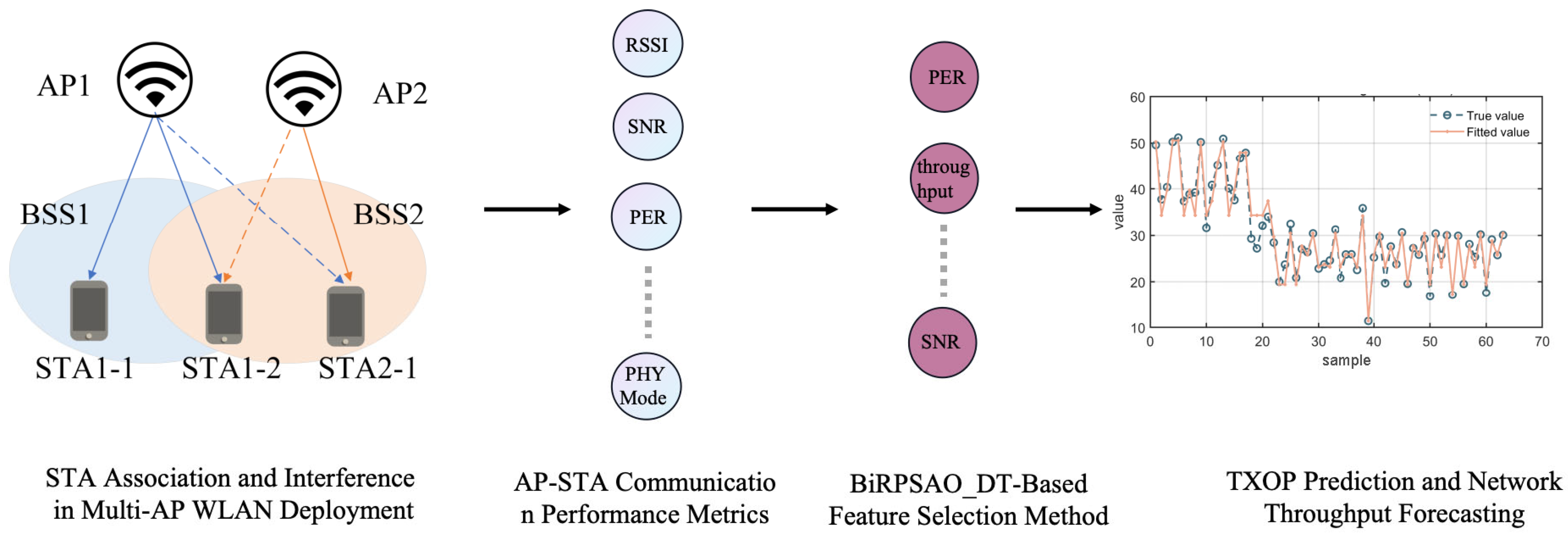
• Joint prediction of TXOP and throughput in dynamic WLAN scenarios: besides traditional throughput modeling, transmission opportunity (TXOP) is introduced as an auxiliary modeling target, constructing a prediction system more aligned with MAC layer transmission mechanisms, thereby better capturing the impact of terminal competition behaviors on bandwidth performance.
• Systematic evaluation on real or simulated datasets: comparative experiments with multiple baseline methods verify the advantages of the proposed method in feature selection efficiency, prediction accuracy, and model stability, demonstrating its practical potential in dynamic wireless environments.

2. Data Preprocessing and Feature Engineering

2.1. Dataset

The dataset used in this study originates from a specific wireless communication testing scenario. The raw data is stored in a structured database format, with key table fields summarized in

Table 1. Dataset label descriptions.

Field Name	Description
test_id	Test ID, used to identify each independent test
test_dur	Test duration (unit: s)
loc_id	Location ID, indicating the area where data collection occurred
protocol	Communication protocol type used (e.g., 802.11n, 802.11ac)
pkt_len	Network packet length (unit: bytes)
bss_id	Basic Service Set Identifier
ap_name	Access Point device name
ap_mac	Access Point MAC address
ap_id	Access Point ID, used to associate with terminals
pd	Preamble length
ed	Extended Detection flag
nav	Network Allocation Vector
eirp	Effective Isotropic Radiated Power
sta_mac	Terminal (STA) MAC address
sta_id	Terminal ID, used to uniquely identify each terminal device
sta_from_sta_0_rssi	RSSI received by STA from STA_0 (unit: dBm)
sta_from_sta_1_rssi	RSSI received by STA from STA_1 (unit: dBm)
nss	Number of Spatial Streams
mcs	Modulation and Coding Scheme number
per	Packet Error Rate
num_ampdu	Number of Aggregated MAC Protocol Data Units (AMPDU)
ppdu_dur	Physical layer Protocol Data Unit (PPDU) duration
other_air_time	Channel occupancy time by other devices
throughput	Network throughput (unit: Mbps)
seq_time	Timestamp sequence corresponding to the current record

. The data primarily includes basic test information, network parameters, device identification details, and statistical features such as an RSSI (Received Signal Strength Indicator), aiming to support subsequent feature extraction, modeling, and analysis.

During data collection, the test network topology is illustrated in Figure 1: under the same frequency band configuration, two Access Points (APs) were deployed, each transmitting downlink data to their associated terminal devices (STAs). The dataset records not only the network topology configuration, traffic load, threshold parameters, and RSSI between nodes but also key frame-level statistical information collected during testing, such as transmission duration per node, modulation and coding scheme (MCS), number of spatial streams (NSS), packet error rate (PER), and actual throughput.

2.2. Label Encoding

Since several variables in the dataset—such as loc_id, protocol, ap_name, ap_mac, ap_id, sta_mac, and sta_id—are in string format, they cannot be directly used for model training and prediction. Therefore, these categorical string variables need to be label encoded. Label encoding maps each unique category to an integer, thereby converting non-numerical data into a numerical form that can be processed by the model.

2.3. Feature Engineering

The features used in this study are shown in Table 1. However, since the RSSI values received by each antenna of the AP are collected every 0.5 s, these signals often contain noise, missing values, and irregular fluctuations. Therefore, it is necessary to preprocess the RSSI information between nodes. This primarily involves extracting statistical features from the received RSSI data. The extracted features include the following ten statistical metrics: maximum, minimum, mean, variance, standard deviation, kurtosis, skewness, rate of change in the RSSI, count of received RSSI values, and the time of RSSI reception.

Except for the count of received RSSI values, the other nine statistical features are extracted using the following methods:

(1)

Maximum (${RSSI}_{max}$)

$${RSSI}_{max}=\max \left(X_i\right)$$

(1)

where X_i represents the sequence of received RSSI values.

(2)

Minimum (${RSSI}_{min}$)

$${RSSI}_{min}=\min \left(X_i\right)$$

(2)

(3)

Mean (${RSSI}_{mean}$)

$${RSSI}_{mean}={\displaystyle \frac{1}{{RSSI}_N}}\sum _{i=1}^N{X}_i$$

(3)

(4)

Variance (${RSSI}_{var}$)

$${RSSI}_{var}={\displaystyle \frac{1}{{RSSI}_N}}\sum _{i=1}^{{RSSI}_N}{\left({X_i-RSSI}_{mean}\right)}^2$$

(4)

(5)

Standard Deviation (${RSSI}_{std}$)

$${RSSI}_{std}=\sqrt{{\displaystyle \frac{1}{{RSSI}_N}}\sum _{i=1}^{{RSSI}_N}{\left({X_i-RSSI}_{mean}\right)}^2}$$

(5)

(6)

Kurtosis (${RSSI}_{kur}$)

$${RSSI}_{kur}={\displaystyle \frac{1}{{RSSI}_N}}\sum _{i=1}^{{RSSI}_N}\left({\displaystyle \frac{{X_i-RSSI}_{mean}}{{RSSI}_{std}}}\right)-3$$

(6)

(7)

Skewness (${RSSI}_{Ske}$)

$${RSSI}_{Ske}={\displaystyle \frac{1}{{RSSI}_N}}\sum _{i=1}^{{RSSI}_N}\left({\displaystyle \frac{{X_i-RSSI}_{mean}}{{RSSI}_{std}}}\right)$$

(7)

(8)

Rate of Change in the RSSI (${RSSI}_{CR}$)

$${RSSI}_{CR}={\displaystyle \frac{X_t-X_{t-1}}{X_{t-1}}}$$

(8)

where $X_t$ is the RSSI value received at time t, and $X_{t-1}$ is the RSSI value collected at time $t-1$.

Reception Time of RSSI:

$${RSSI}_{time}={RSSI}_N\times 0.5$$

(9)

Through feature extraction, excluding the test ID (test_id), the features from two wireless receiving points total 221 dimensions, while the features from three wireless receiving points total 334 dimensions.

3. Method

This paper proposes a feature selection and modeling method that integrates the Snow-Melting Optimizer (SMO) with decision regression models, aiming to improve the prediction accuracy of transmission opportunity (TXOP) and throughput in WLANs. The method first performs a global search in the high-dimensional feature space using the SMO to efficiently select a subset of features that critically contribute to prediction performance. Subsequently, the selected feature subset is fed into multiple ensemble regression models for parallel modeling and joint prediction. This approach combines the accuracy of feature selection with the robustness of modeling and prediction. The overall process is illustrated in Figure 2.

3.1. Binary Random Pruning Snow Melting Optimizer with Decision Tree (BiRPSMO-DT)

Wrapper feature selection is regarded as a combinatorial optimization problem, where different subsets of features yield different scores using the same regression method. In this problem, each feature has two states: selected (represented as 1) or not selected (represented as 0). Since the SMO algorithm initializes individuals in a continuous space, the magnitude and range of feature values need to be considered, especially when dealing with large-scale datasets, which can lead to higher computational costs. In contrast, a binary population can more directly represent the solution space of the problem, enabling efficient searching within the feature subset space to find the optimal feature combination.

This study employs the Sigmoid function to map the SMO algorithm’s population from continuous space to a binary search space to explore feature subsets. The subsets are then evaluated using a decision tree (DT) to identify the optimal feature subset, thereby addressing the feature selection problem and improving the model’s generalization capability.

(1)

Binary Population Initialization

This paper uses the S-shaped function to transform the continuous space into a binary search space for population initialization. The S-shaped function maps values from the continuous space to the range between 0 and 1. The purpose of this transformation function is to convert continuous values into binary values. In BiRPSMO, the binary solution space is represented by an N × D matrix, where N is the population size and D is the dimensionality of the dataset. Values of 1 and 0, respectively, indicate that a feature is selected or not selected. The expression of the Sigmoid function is shown in Equation (10), illustrating the output of the S-shaped function in a continuous form.

$$X_{s_i}^k\left(t\right)={\displaystyle \frac{1}{1+e^{-X_i^k\left(t\right)}}}$$

(10)

where $X_i^k\left(t\right)$ represents the k dimension of the i particle at iteration t.

For the feature selection problem, introducing a certain degree of randomness can enhance the diversity and robustness of the search process. Therefore, the S-shaped function is combined with random perturbation, that is, a certain amount of random disturbance is added to the output value of the S-shaped function. This can be expressed as follows:

$$X_{s_i}^k\left(t\right)={\displaystyle \frac{1}{1+e^{-R_B{X}_i^k\left(t\right)}}}$$

(11)

where $R_B$ is a D random perturbation.

(2)

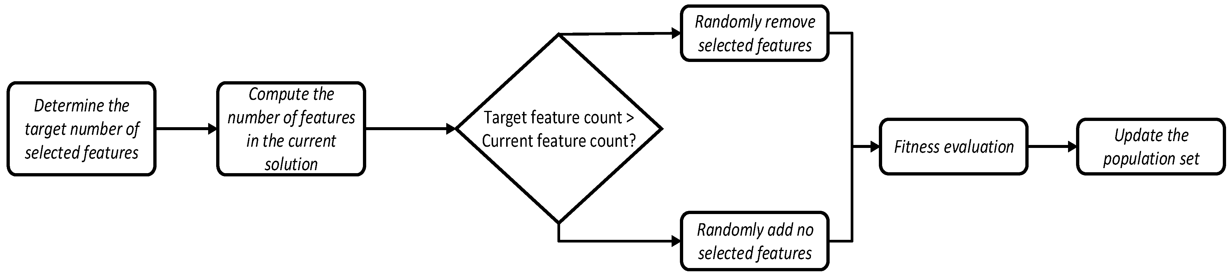
Population Constraint Strategy Based on Random Pruning

Meanwhile, a population constraint strategy based on random pruning is proposed. This strategy limits the updated population to ensure that the number of selected individuals equals the desired number of target features. The process of the random pruning strategy is illustrated in Figure 3.

Specific implementation process of the algorithm:

• Obtain the target number of features: First, retrieve the desired number of features num_features from the input parameters.
• Convert to binary representation: The population is converted into a binary representation, where each individual is represented as a binary string of length Dim, with Dim denoting the total number of features. In this binary string, each bit corresponds to a specific feature: a value of 1 indicates that the feature is selected, while a value of 0 means the feature is not selected.
• Calculate the number of selected features: Select the top 50% of individuals based on fitness and compute the number of selected features (select_features) for each individual.
• Adjust the number of features: If the number of selected features for any individual exceeds num_features, adjustment is required:
  If select_features > num_features, randomly deselect (select_features − num_features) features.
  If select_features < num_features, randomly select (num_features − select_features) additional features.
• Update the population: Based on the adjustments, update each individual’s representation in the population to ensure all individuals satisfy the constraint.

This random pruning constraint strategy ensures that the number of features selected by each solution generated during the BiRPSMO algorithm’s search process matches the required target number. It effectively narrows the search space and improves the algorithm’s performance and stability.

(3)

Fitness Function

Feature selection can be regarded as a combinatorial optimization problem, where meta-heuristic methods are employed as approximate solutions to find the optimal or near-optimal subset of features. To guide the optimization process effectively, it is essential to define an appropriate objective function that serves as the evaluation criterion during algorithm iterations. The objective function is defined as shown in Equation (12):

$${Fitness}_{regression}=\omega ({\displaystyle \frac{1}{N}}\sum _{i=1}^N{\left(y_i-\widehat{y_i}\right)}^2)+(1-\omega ){\displaystyle \frac{SF}{TF}}$$

(12)

(4)

Snow Ablation Optimizer Algorithm Process

In each generation of the SMO algorithm, new candidate solutions are generated based on the current feature subsets, and the best solution is updated by evaluating the performance of the wide learning system on these candidates. Through continuous iterative optimization, the final best solution represents the optimal feature subset along with the corresponding performance of the wide learning system. The specific algorithm process is as follows (Algorithm 1):

Algorithm 1: Feature Selection Based on BiRPSMO and DT

Definitions: Population size $X_i\left(i=\mathrm{1,2},\dots ,N\right)$, feature dimension Dim, iteration coun $t=0$, maximum iterations $t_{max}$, two subpopulations $N_a=N_b={\displaystyle \frac{N}{2}}$, optimal feature set $S_f=\mathrm{\varnothing }$, elite pool Elite = $\varnothing$. Steps: 1. Initialize the population (snow pile) X as N individuals of Dim-dimensional binary strings, and the best position G(t). 2. Apply constraints to the population. 3. Calculate the initial population’s objective function values using DT and record the best individual G(t). 4. Rank individuals by score and build the elite pool Elite(t). 5. While t < $t_{max}$, do:    5.1 Calculate snow melting rate M and the centroid of the population $\overline{X}\left(t\right)$ according to Formulas (10) and (6).    5.2 Randomly divide the population into two groups $P_a$ and $P_b$.    5.3 Update Pa based-on Elite(t), G(t), $\overline{X}\left(t\right)$, and the S-shaped transfer function.    5.4 Adjust Pa and Pb according to Formula (13).    5.5 Update Pb based on $G\left(t\right)$, $\overline{X}\left(t\right)$, and the S-shaped function.    5.6 Recalculate objective scores of the updated population; if improved, update best score and position.    5.7 Update Elite(t).    5.8 t = t + 1. 6. End. 7. Return the best position G(t). 8. Map the best position back to the binary population and select features $S_f$. 9. Output the feature subset $S_f$.

3.2. Decision Tree Regression

Decision Tree Regression is a nonlinear supervised learning method based on a tree structure. Its core idea is to recursively partition the data into multiple subregions and fit a constant value in each region to perform the prediction task. The entire tree consists of a series of nodes and branches: each internal node corresponds to a decision rule based on a feature; each branch represents a value range or condition for that feature; and the leaf nodes represent the final prediction output.

Depending on the splitting criteria and application tasks, decision tree algorithms come in several variants, such as ID3 (Iterative Dichotomiser 3), C4.5, CART (Classification and Regression Tree), and MARS (Multivariate Adaptive Regression Splines). Among them, ID3 and C4.5 build multi-way classification trees and are suitable for classification tasks with discrete labels, whereas the CART algorithm supports building both classification and regression trees, making it one of the most widely used methods for regression tasks.

In CART regression trees, the model selects the best splitting feature and split point by minimizing the Mean Squared Error (MSE) within the nodes. It then recursively splits the data in a binary fashion until a stopping condition is met. Unlike classification trees that use metrics like the Gini index or information gain, regression trees use variance or prediction error as the splitting criterion, ensuring that the samples in each leaf node are as similar as possible.

$$in=({\displaystyle \frac{1}{2n}}{\sum }_{i=1}^n\left(y_i-X_i\beta {)}^2+\lambda \parallel \beta {\parallel }_1\right)$$

(13)

where n is the number of samples; $y_i$ is the response value of the sample i; $X_i$ is the feature vector of the i sample; and $\lambda$ is the regularization parameter that controls the strength of the L1 regularization. ${‖\beta ‖}_1$ denotes the L1 norm. In this objective function, the first term is the loss function (mean squared error), and the second term is the L1 regularization term, which aims to achieve feature selection by penalizing large coefficients. By choosing an appropriate value for $\lambda$, the sparsity of the features can be controlled, thereby enabling feature selection.

4. Results and Discussion

The parameters used for feature selection and regression models are summarized in

Table 2. Parameter settings for different algorithms and models.

Model	Hyperparameters
Genetic Algorithm (GA)	Crossover rate = 0.8; Mutation rate = 0.1
Particle Swarm Optimization (PSO)	Cognitive coefficient (c1) = 0.5; Social coefficient; (c2) = 0.3; Inertia weight (ω) = 0.9
Snow Melting Algorithm (SMO)	Elite pool size = 0.5 × N
BiRPSMO	Elite pool size = 0.5 × N
Multiple Linear Regression	Intercept term enabled (fit_intercept = True)
LASSO Regression	Regularization parameter (alpha) = 1.0 Intercept term enabled (fit_intercept = True)
Ridge Regression	Regularization parameter (alpha) = 1.0 Intercept term enabled (fit_intercept = True)
Decision Tree Regression	Minimum samples per leaf = 1
Random Forest Regression	Number of trees = 100; Minimum samples per leaf = 1
XGBoost Regression	Number of weak learners = 100; Learning rate = 0.3

. For the feature selection task, the maximum number of iterations (t) for the GA [23], PSO [24], SMO, and the hybrid algorithm BiRPSMO was uniformly set to 100, with a population size (N) of 30. To reduce the impact of randomness on the results, all optimization algorithms and regression models were independently executed 10 times under identical parameter settings. The average performance over these runs was then evaluated and compared.

4.1. Feature Selection

The experimental results shown in

Table 3. Performance comparison of different feature selection methods.

Model	MAE	MAPE	MSE	RMSE	R2	Number of Selected Features
GA_DT	2.1866	6.5722	13.1898	3.6318	0.8830	96
PSO_DT	2.1947	6.5835	13.7231	3.7045	0.8782	109
BiSMO_DT	2.3524	7.4458	15.8739	3.9842	0.8592	39
BiRPSMO_DT	1.9141	5.7604	11.2816	3.3588	0.8999	44

demonstrate significant differences in prediction performance and feature dimension control when applying different feature selection methods within the decision tree model. Overall, the BiRPSMO_DT model achieves the best performance across all evaluation metrics, with a mean absolute error (MAE) of 1.9141, mean absolute percentage error (MAPE) of 5.7604, mean squared error (MSE) of 11.2816, root mean squared error (RMSE) of 3.3588, and a coefficient of determination (R²) reaching 0.8999, while selecting only 44 features. This demonstrates a good balance between predictive accuracy and feature compression. In comparison, although GA_DT and PSO_DT maintain relatively high R² values (0.8830 and 0.8782, respectively), their error metrics are slightly higher, and they select more features—96 and 109, respectively—indicating lower feature selection efficiency than BiRPSMO_DT. BiSMO_DT controls the number of selected features well by retaining only 39 features but exhibits relatively lower predictive accuracy, with an MAE of 2.3524 and R² dropping to 0.8592, indicating that it loses considerable useful information while compressing features. In summary, BiRPSMO_DT significantly improves model prediction performance while maintaining fewer selected features, proving its superior feature selection capability for device identification and signal feature data, making it the optimal feature selection method for this task.

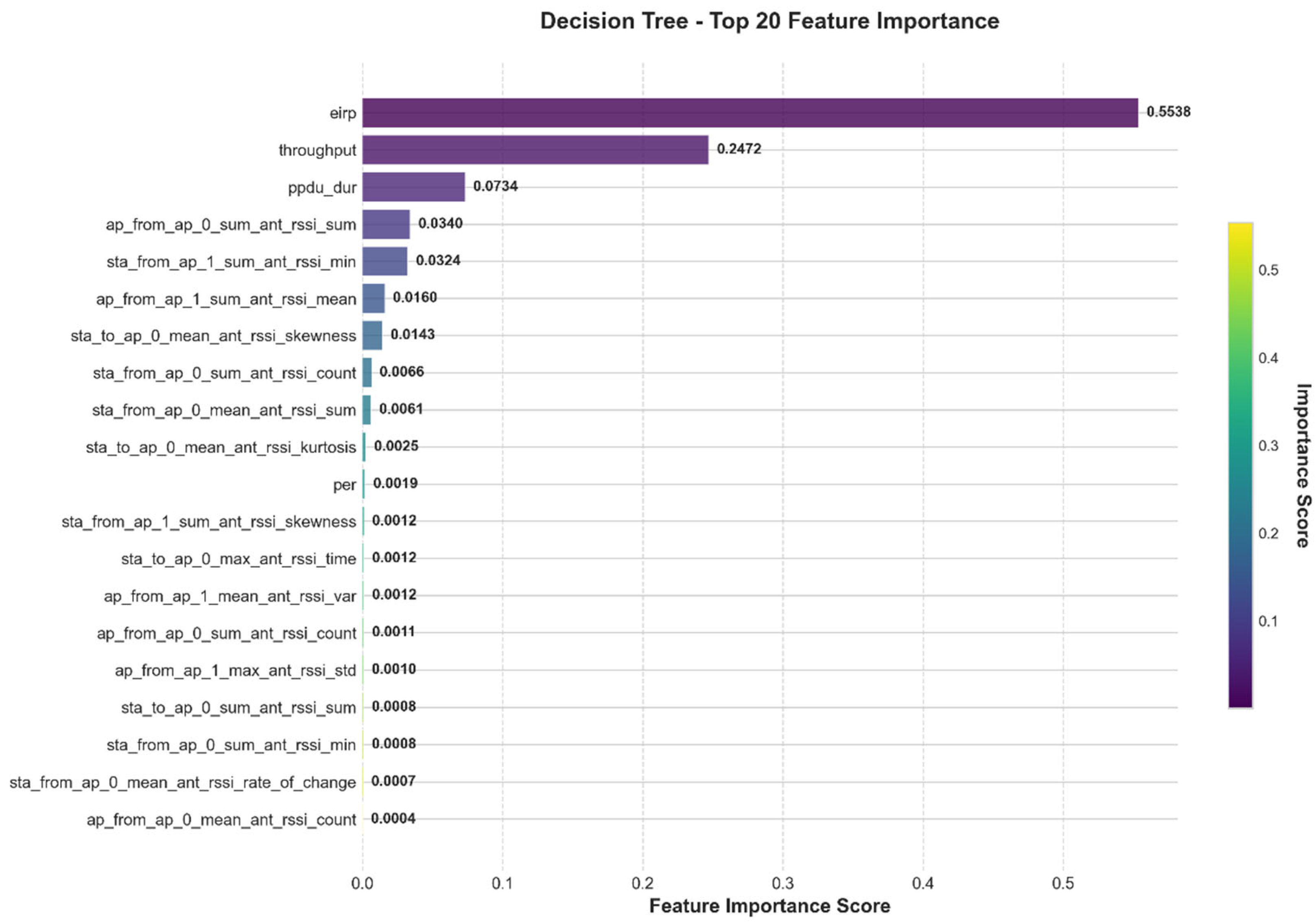
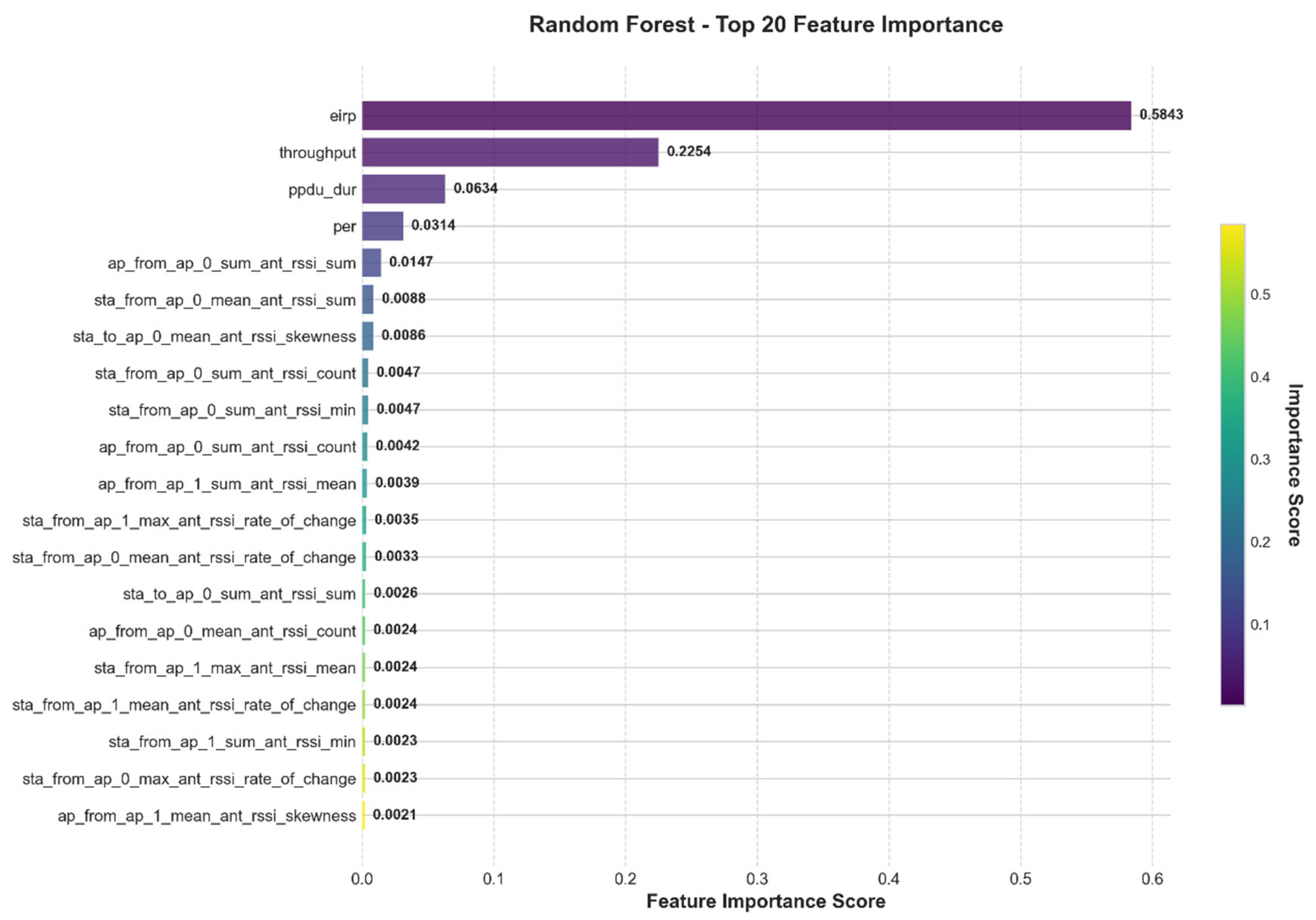
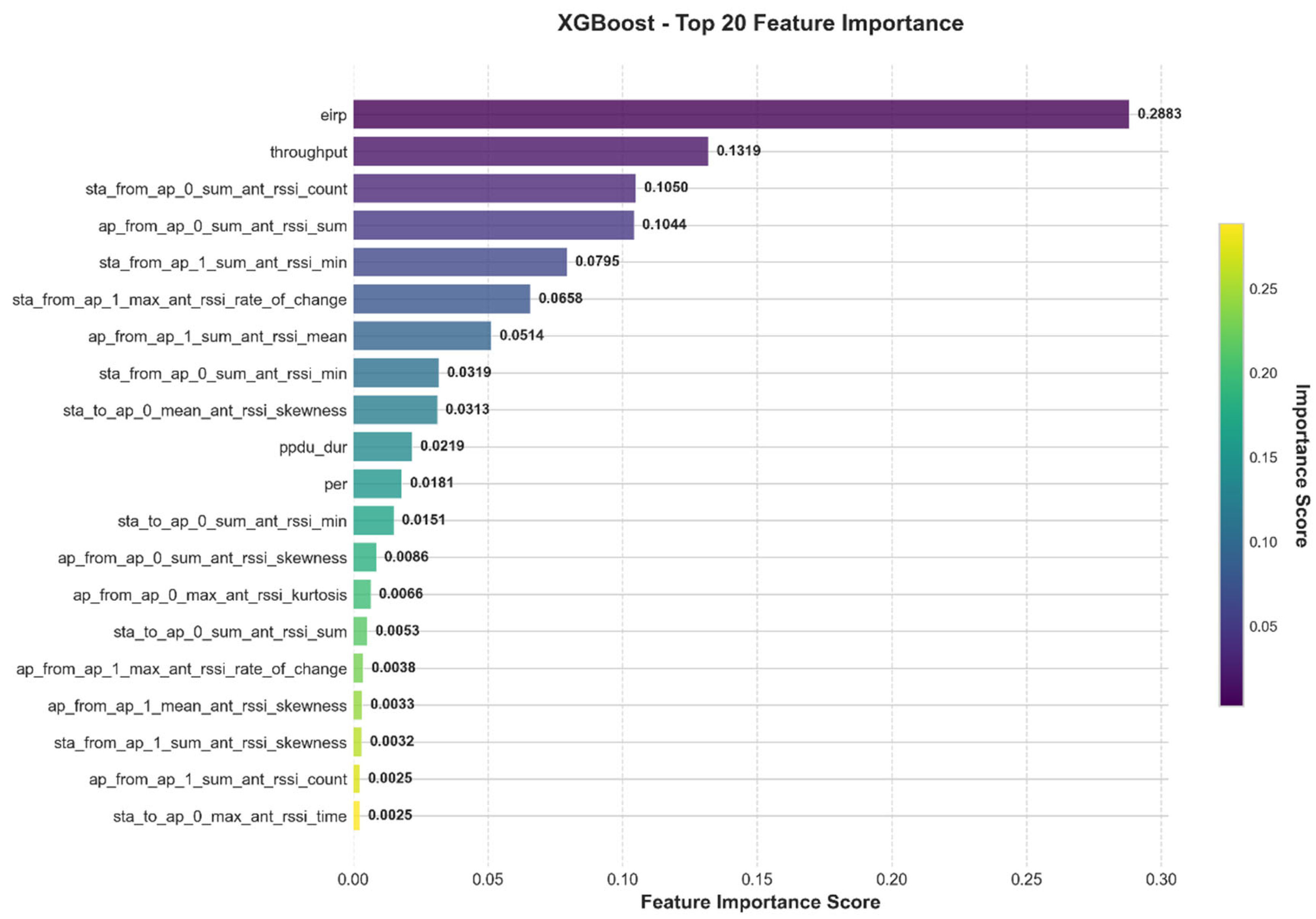
4.2. Feature Contribution

Based on the data obtained from the previous feature selection, Decision Tree, Random Forest, and XGBoost methods were used, respectively, to analyze the feature contributions of wireless network performance characteristics. The analysis results are shown in Figure 4, Figure 5, Figure 6 and Figure 7.

From the feature importance analysis results, eirp (Equivalent Isotropically Radiated Power) demonstrates significant importance across all three models, serving as a core variable influencing model prediction performance. In the Decision Tree, Random Forest, and XGBoost models, the feature importance of eirp is 0.5538, 0.5843, and 0.2883, respectively, all markedly higher than other features. This indicates its dominant role in device identification and wireless signal modeling. This finding also confirms the fundamental impact of transmission power on signal quality and reception performance in wireless communication systems.

Throughput ranks as the second most important feature across all three models, with importance values of 0.2472 in Decision Tree, 0.2254 in Random Forest, and 0.1319 in XGBoost. This indicates that throughput also has strong explanatory power for system performance and may reflect the intrinsic relationship between device communication quality and stability. Additionally, the models differ in their sensitivity to other features. Both the Decision Tree and Random Forest methods identify ppdu_dur (PPDU duration) as the third most important feature, highlighting its strong discriminative ability in traditional information gain-based tree models. In contrast, the XGBoost model assigns relatively higher weights to RSSI-related features such as sta_from_ap_0_sum_ant_rssi_count, ap_from_ap_0_sum_ant_rssi_sum, and sta_from_ap_1_sum_ant_rssi_min, suggesting that the gradient boosting mechanism is better at capturing nonlinear patterns in RSSI statistical features. Looking at overall statistics, the average feature importance across the three models is 0.0227, but the standard deviations differ: Decision Tree (0.0896) and Random Forest (0.0923) are relatively high, whereas XGBoost’s standard deviation is 0.0514. This implies that XGBoost distributes importance more evenly, showing a more balanced reliance on multiple features and potentially stronger generalization capability.

Overall, eirp and throughput are consistently recognized as key features across models, indicating their high stability and broad applicability. In contrast, the importance of the RSSI and its statistical derivatives is more influenced by the model structure, showing especially strong performance in ensemble-based models.

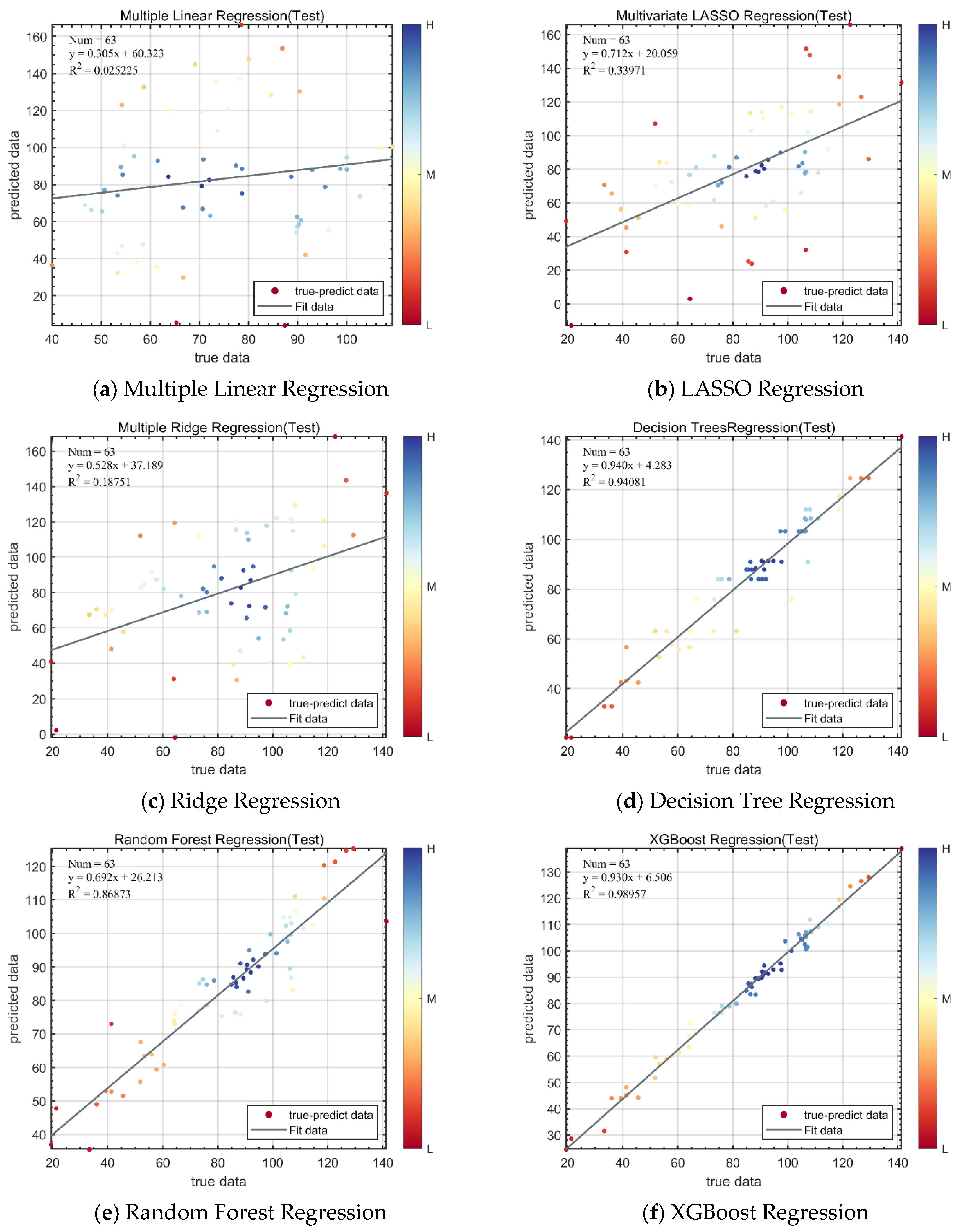
4.3. Transmission Opportunity Prediction

This study employs multiple linear regression, LASSO Regression, Ridge Regression, Decision Tree Regression, Random Forest Regression, and XGBoost Regression to build prediction models. The fitted plots and evaluation results of each model are shown in Figure 8 and

Table 4. Evaluation metrics of the 2AP model predictions.

Model	MAE	MAPE	MSE	RMSE	R2
Multiple Linear Regression	3.321	0.11569	17.292	4.1584	0.80155
LASSO Regression	3.321	0.11571	17.2848	4.1575	0.80164
Ridge Regression	3.3392	0.11782	16.7709	4.0952	0.80753
Decision Tree Regression	1.3623	0.046989	4.3808	2.093	0.94973
Random Forest Regression	2.0796	0.084708	7.0621	2.6575	0.91895
XGBoost Regression	0.9016	0.035258	1.3746	1.1724	0.98422

.

As shown in Figure 8 and Table 4, the six regression models exhibit notable differences in prediction accuracy based on various evaluation metrics (MAE, MAPE, MSE, RMSE, R²). The traditional linear models—Multiple Linear Regression, LASSO Regression, and Ridge Regression—demonstrate relatively weaker overall performance, with R² values around 0.80, indicating that they can explain approximately 80% of the variance in the target variable. Among them, Ridge Regression slightly outperforms the others in terms of MSE and R², suggesting its advantage in handling multicollinearity.

In contrast, tree-based methods significantly improve model fitting capabilities. Decision Tree Regression achieves lower MAE and RMSE values of 1.3623 and 2.093, respectively, with an R² of 0.94973, demonstrating strong capacity in modeling nonlinear relationships. However, its relatively limited generalization ability may pose a risk of overfitting, especially when dealing with small sample sizes or complex feature spaces.

Random Forest Regression outperforms linear models across all metrics and effectively mitigates the overfitting risk associated with a single decision tree. With an R² of 0.91895 and substantially reduced prediction errors, it showcases the robustness and strong generalization capability of ensemble learning methods.

Among all models, XGBoost Regression delivers the best performance. It achieves the lowest MAE of 0.9016, MAPE of 0.035258, and MSE and RMSE values of 1.3746 and 1.1724, respectively, with a remarkably high R² of 0.98422. These results indicate that XGBoost nearly perfectly fits the data. By integrating regularization, automatic feature selection, and weighted boosting mechanisms, XGBoost not only prevents overfitting but also significantly enhances model expressiveness.

In summary, although linear models offer advantages in interpretability, they are limited in modeling complex relationships. Tree-based models and ensemble methods—especially XGBoost—demonstrate excellent performance in terms of both fitting accuracy and stability, making them the preferred approach for this type of prediction task. The experimental results confirm that XGBoost regression can effectively enhance the prediction accuracy of AP transmission opportunities.

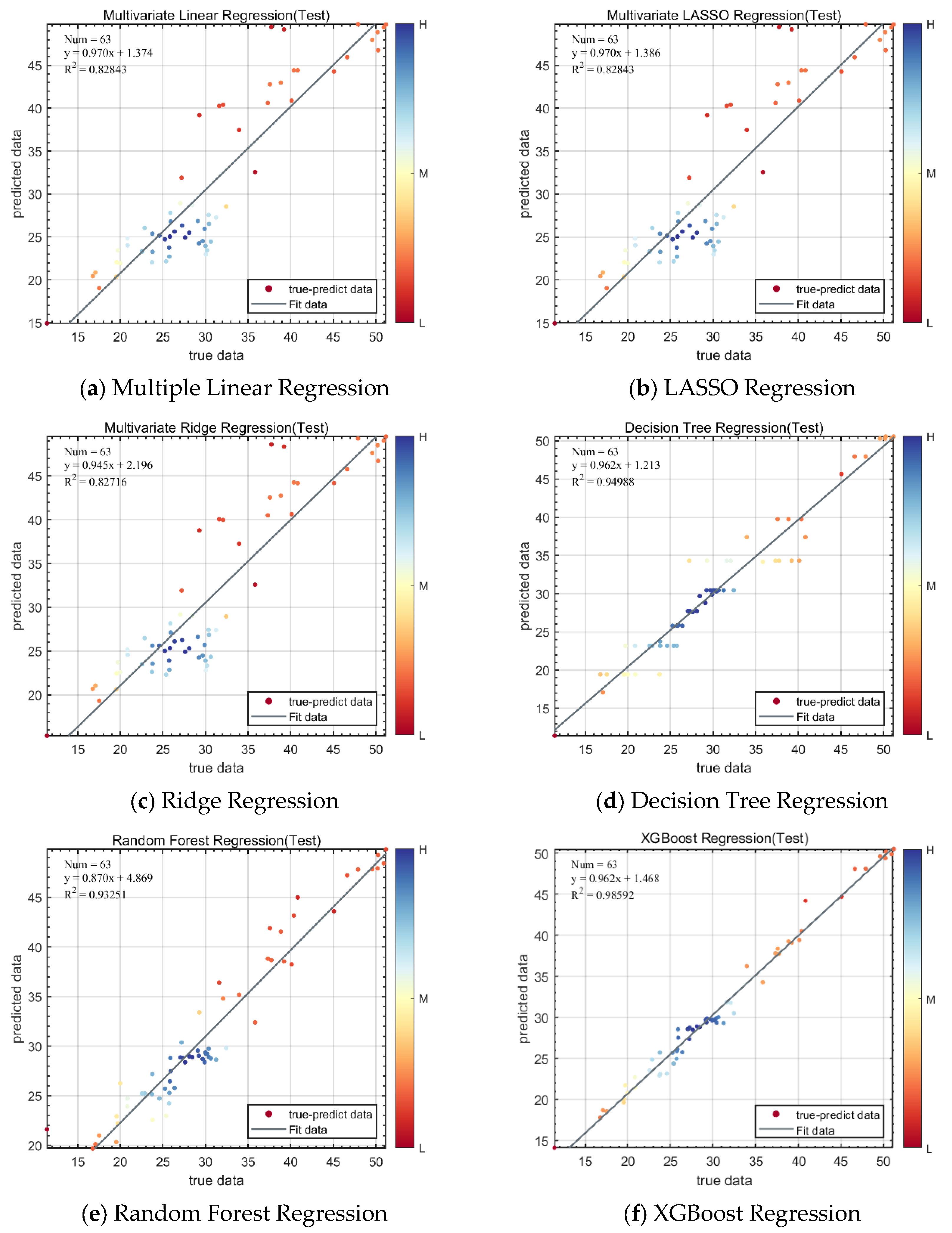
4.4. AP Throughput and Bandwidth Prediction

This section builds models to predict the uplink and downlink bandwidth of the transmitting AP using six regression algorithms—Multiple Linear Regression [25], LASSO Regression [26], Ridge Regression [27], Decision Tree Regression [28], Random Forest Regression [29], and XGBoost Regression [30]—based on the selected features. The performance of each regression model is comprehensively evaluated using three metrics: Mean Squared Error (MSE), Root Mean Squared Error (RMSE), and the coefficient of determination (R²), The relevant experimental results are shown in Figure 9.

As shown in

Table 5. Throughput prediction results under 2-AP scenario.

Model	MAE	MAPE	MSE	RMSE	R2
Multiple Linear Regression	22.624	0.32647	808.9904	28.4428	0.025225
LASSO Regression	22.7191	0.32735	809.9635	28.45999	0.33971
Ridge Regression	27.0598	0.37995	1066.7536	32.6612	0.18751
Decision Tree Regression	4.6083	0.062756	44.5059	6.6713	0.94081
Random Forest Regression	8.0441	0.13538	124.2838	11.1483	0.86873
XGBoost Regression	2.5071	0.043215	10.8037	3.2869	0.98957

, the comparison of prediction performances across multiple regression models reveals significant differences in their ability to predict throughput. Among the traditional linear models, both Multiple Linear Regression and LASSO Regression exhibit relatively large prediction errors, with MAE values above 22 and R² values of 0.0252 and 0.3397, respectively, indicating limited explanatory power for throughput. This limitation likely stems from the complex nonlinear relationships among features involved in throughput prediction, which exceed the fitting capacity of linear models. Ridge regression performs even worse, with an RMSE of 32.66 and R² of 0.1875, possibly due to its sensitivity to outliers or overly strong regularization.

In contrast, ensemble learning algorithms show much better performance. Decision Tree Regression stands out with an R² of 0.9408, meaning it can explain the majority of data variance. Its MAE is only 4.61 and RMSE just 6.67, demonstrating strong fitting accuracy. However, single trees are prone to overfitting, so the model’s generalization ability requires further validation. Random forest regression significantly improves stability and generalization; although its MAE (8.04) is slightly higher than that of the decision tree, its overall RMSE (11.15) and R² (0.8687) still indicate solid performance. As a model combining multiple decision trees, Random Forest effectively handles nonlinear feature interactions and noise robustness.

The best performing model is XGBoost regression, which achieves the top scores across all metrics: MAE of only 2.51, MAPE of 0.0432, MSE of 10.80, and an R² as high as 0.9896. This indicates near-perfect fitting on the training data. By leveraging gradient boosting and regularization techniques, XGBoost effectively enhances both accuracy and robustness, making it especially suitable for datasets with complex relationships and numerous features.

4.5. Discussion

The experimental results, presented in Table 4 and Table 5, correspond to the prediction of WLAN transmission opportunity and throughput, respectively. Among the evaluated models, the XGBoost Regression model consistently outperforms others across all metrics, demonstrating lower prediction errors and better fitting performance. This superiority mainly stems from XGBoost’s use of the gradient boosting tree method, which effectively captures complex nonlinear relationships in the data through iterative weak learners. Its built-in regularization mechanism helps prevent overfitting, thereby enhancing model stability and generalization capability. Additionally, XGBoost’s automatic handling of missing values and efficient computational performance enable it to achieve stronger predictive accuracy and practicality when dealing with complex tasks influenced by multiple factors, such as WLAN throughput and transmission opportunity prediction. Although the methods proposed in this study have achieved good performance in transmission opportunity and throughput prediction tasks, there are still some limitations. First, the feature selection process relies on the global search capability of SAO, whose convergence speed and stability may be affected when dealing with larger-scale datasets. Second, this study mainly evaluates static datasets and has yet to consider modeling requirements for dynamic scenarios in real WLANs. Moreover, some model parameters were not automatically tuned during training, which might impact the final prediction performance. Future work could further incorporate adaptive parameter optimization strategies combined with time-series modeling methods to enhance the model’s generalization ability and real-time prediction performance in practical network environments.

In addition, correlation analysis (see Figure 4, Figure 5, Figure 6 and Figure 7) indicates that transmission opportunity and throughput exhibit a nonlinear or weak correlation. This suggests that in certain cases, even with sufficient transmission opportunities, overall throughput may still decline due to deteriorated channel conditions, frequent collisions, or inefficient resource scheduling, reflecting a complex coupling relationship between the two. Further analysis shows that among all influencing factors, Equivalent Isotropically Radiated Power (eirp) demonstrates the strongest correlation with network throughput, indicating that signal transmission strength has a significant impact on overall data transmission performance.

5. Conclusions

This paper proposes a feature selection and modeling method that integrates the Snow Melt Optimizer (SMO) with a Decision Tree Regression model to predict transmission opportunities and throughput in WLANs. Experimental results show that this method can significantly reduce feature dimensionality while maintaining high prediction accuracy. Notably, after employing the XGBoost model, all performance metrics outperform traditional methods, validating the effectiveness and reliability of this approach in handling high-dimensional network data and modeling complex relationships.

6. Limitations and Future Work

The proposed method shows good results but still has some limitations. In this paper, “static scenarios” means the Sta devices stay in fixed positions and do not move. First, the feature selection method based on the Snow Melt Optimizer (SMO) may have slower convergence and less stability when working with larger datasets. Further theoretical analysis and experimental validation are needed to study this problem and find other solutions. Second, our experiments use only static datasets. We have not fully considered dynamic scenarios where Sta devices move. The effects of device movement on the channel, multipath, and model performance need to be explained more clearly. In future work, we will combine spatiotemporal feature analysis with trajectory prediction. This will help improve the model’s ability to adapt and predict in real time for dynamic WLAN environments. It will also better support network resource allocation and service quality.

References

1. Gao, D.; Wang, H.; Chen, Y.; Ye, Q.; Wang, W.; Guo, X.; Wang, S.; Liu, Y.; He, T. LoBee: Bidirectional Communication between LoRa and ZigBee based on Physical-Layer CTC. IEEE Trans. Wirel. Commun. 2025. [Google Scholar] [CrossRef]
2. Wilhelmi, F.; Barrachina-Muñoz, S.; Bellalta, B.; Cano, C.; Jonsson, A.; Ram, V. A flexible machine-learning-aware architecture for future WLANs. IEEE Commun. Mag. 2020, 58, 25–31. [Google Scholar] [CrossRef]
3. Pan, D. Analysis of Wi-Fi Performance Data for a Wi-Fi Throughput Prediction Approach. 2017. Available online: https://www.diva-portal.org/smash/record.jsf?pid=diva2:1148996 (accessed on 4 November 2024).
4. Lee, C.; Abe, H.; Hirotsu, T.; Umemura, K. Analytical modeling of network throughput prediction on the internet. IEICE Trans. Inf. Syst. 2012, 95, 2870–2878. [Google Scholar] [CrossRef]
5. Venkatachalam, I.; Palaniappan, S.; Ameerjohn, S. Compressive sector selection and channel estimation for optimizing throughput and delay in IEEE 802.11 ad WLAN. Int. J. Inf. Technol. 2025, 17, 987–998. [Google Scholar]
6. Zhang, J.; Han, G.; Qian, Y. Queuing theory based co-channel interference analysis approach for high-density wireless local area networks. Sensors 2016, 16, 1348. [Google Scholar] [CrossRef] [PubMed]
7. Oghogho, I.; Edeko, F.O.; Emagbetere, J. Measurement and modelling of TCP downstream throughput dependence on SNR in an IEEE802. 11b WLAN system. J. King Saud Univ.Eng. Sci. 2018, 30, 170–176. [Google Scholar] [CrossRef]
8. Khan, M.A.; Hamila, R.; Al-Emadi, N.A.; Kiranyaz, S.; Gabbouj, M. Real-time throughput prediction for cognitive Wi-Fi networks. J. Netw. Comput. Appl. 2020, 150, 102499. [Google Scholar] [CrossRef]
9. Divya, C.; Naik, P.V.; Mohan, R. Throughput Analysis of Dense-Deployed WLANs Using Machine Learning. In Proceedings of the 2023 International Conference on Advances in Electronics, Communication, Computing and Intelligent Information Systems (ICAECIS), Bangalore, India, 19–21 April 2023; IEEE: Piscataway, NJ, USA, 2023; pp. 332–337. [Google Scholar]
10. Szott, S.; Kosek-Szott, K.; Gawłowicz, P.; Gómez, J.T.; Bellalta, B.; Zubow, A.; Dressler, F. Wi-Fi meets ML: A survey on improving IEEE 802.11 performance with machine learning. IEEE Commun. Surv. Tutor. 2022, 24, 1843–1893. [Google Scholar] [CrossRef]
11. Ali, R.; Nauman, A.; Zikria, Y.B.; Kim, B.-S.; Kim, S.W. Performance optimization of QoS-supported dense WLANs using machine-learning-enabled enhanced distributed channel access (MEDCA) mechanism. Neural Comput. Appl. 2020, 32, 13107–13115. [Google Scholar] [CrossRef]
12. Shao, S.; Fan, M.; Yu, C.; Li, Y.; Xu, X.; Wang, H. Machine Learning-Assisted Sensing Techniques for Integrated Communications and Sensing in WLANs: Current Status and Future Directions. Prog. Electromagn. Res. 2022, 175, 45–79. [Google Scholar] [CrossRef]
13. Shaabanzadeh, S.S.; Sánchez-González, J. Contribution to the Development of Wi-Fi Networks Through Machine Learning Based Prediction and Classification Techniques. Ph.D. Thesis, Universitat Politècnica de Catalunya Barcelona, Barcelonam, Spain, 2024. [Google Scholar]
14. Feng, Y.; Liu, L.; Shu, J. A link quality prediction method for wireless sensor networks based on XGBoost. IEEE Access 2019, 7, 155229–155241. [Google Scholar] [CrossRef]
15. Sheng, C.; Yu, H. An optimized prediction algorithm based on XGBoost. In Proceedings of the 2022 International Conference on Networking and Network Applications (NaNA), Urumchi, China, 3–5 December 2022; IEEE: Piscataway, NJ, USA, 2002; pp. 1–6. [Google Scholar]
16. Mohan, R.; Ramnan, K.V.; Manikandan, J. Machine Learning approaches for predicting Throughput of Very High and EXtreme High Throughput WLANs in dense deployments. In Proceedings of the 2021 12th International Conference on Computing Communication and Networking Technologies (ICCCNT), Kharagpur, India, 6–8 July 2021; IEEE: Piscataway, NJ, USA, 2021; pp. 1–6. [Google Scholar]
17. Min, G.; Hu, J.; Jia, W.; Woodward, M.E. Performance analysis of the TXOP scheme in IEEE 802.11 e WLANs with bursty error channels. In Proceedings of the 2009 IEEE Wireless Communications and Networking Conference, Budapest, Hungary, 5–8 April 2009; IEEE: Piscataway, NJ, USA, 2009; pp. 1–6. [Google Scholar]
18. Vergara, J.R.; Estévez, P.A. A review of feature selection methods based on mutual information. Neural Comput. Appl. 2014, 24, 175–186. [Google Scholar] [CrossRef]
19. Fernandez, G.A. Machine Learning for Wireless Network Throughput Prediction. Adv. Mach. Learn. Artif. Intell. 2023, 5, 1–6. [Google Scholar]
20. Zhao, X.; Liu, W. Artificial Intelligence Based Feature Selection and Prediction of Downlink IP Throughput. In Proceedings of the 2023 International Conference on Wireless Communications and Signal Processing (WCSP), Hangzhou, China, 2–4 November 2023; IEEE: Piscataway, NJ, USA, 2023; pp. 116–121. [Google Scholar]
21. Jiwane, U.B.; Jugele, R.N. A Hybrid Swarm Intelligence Technique for Feature Selection in Support Vector Machine (SVM) Classifier using Particle Swarm Optimization (PSO) and Ant Colony Optimization (ACO). Cureus J. 2025, 2. [Google Scholar] [CrossRef]
22. Deng, L.; Liu, S. Snow ablation optimizer: A novel metaheuristic technique for numerical optimization and engineering design. Expert Syst. Appl. 2023, 225, 120069. [Google Scholar] [CrossRef]
23. Mirjalili, S. Genetic algorithm. In Evolutionary Algorithms and Neural Networks: Theory and Applications; Springer: Cham, Switzerland, 2019; pp. 43–55. [Google Scholar]
24. Wang, D.; Tan, D.; Liu, L. Particle swarm optimization algorithm: An overview. Soft Comput. 2018, 22, 387–408. [Google Scholar] [CrossRef]
25. Tranmer, M.; Elliot, M. Multiple linear regression. Cathie Marsh Cent. Census Surv. Res. 2008, 5, 1–5. [Google Scholar]
26. Ranstam, J.; Cook, J.A. LASSO regression. J. Br. Surg. 2018, 105, 1348. [Google Scholar] [CrossRef]
27. McDonald, G.C. Ridge regression. Wiley Interdiscip. Rev. Comput. Stat. 2009, 1, 93–100. [Google Scholar] [CrossRef]
28. Fürnkranz, J. Decision Tree. In Encyclopedia of Machine Learning; Sammut, C., Webb, G.I., Eds.; Springer: Boston, MA, USA, 2010; pp. 263–267. [Google Scholar]
29. Segal, M.R. Machine Learning Benchmarks and Random Forest Regression. Center for Bioinformatics and Molecular Biostatistics. 2004. Available online: https://escholarship.org/uc/item/35x3v9t4#author (accessed on 20 July 2025).
30. Chen, T.; Guestrin, C. Xgboost: A scalable tree boosting system. In Proceedings of the 22nd Acm Sigkdd International Conference on Knowledge Discovery and Data Mining, San Francisco, CA, USA, 13–17 August 2016; pp. 785–794. [Google Scholar]
Figure 1. Schematic diagram of wireless dataset feature collection.
Electronics 14 02941 g001
Figure 2. Proposed method in this study.
Electronics 14 02941 g002
Figure 3. The process of handling population constraints.
Electronics 14 02941 g003
Figure 4. Feature contribution results of decision tree.
Electronics 14 02941 g004
Figure 5. Feature contribution results of random forest.
Electronics 14 02941 g005
Figure 6. Feature contribution results of XGBoost.
Electronics 14 02941 g006
Figure 7. Comparison of feature importance across Decision Tree, Random Forest, and XGBoost methods.
Electronics 14 02941 g007
Figure 8. Fitting results of the 2-AP transmission opportunity prediction models.
Electronics 14 02941 g008
Figure 9. Fitting results of the AP throughput and bandwidth prediction models.
Electronics 14 02941 g009