SVRG-AALR: Stochastic Variance-Reduced Gradient Method with Adaptive Alternating Learning Rate for Training Deep Neural Networks

Abstract

The stochastic variance-reduced gradient (SVRG) theory is particularly well-suited for addressing gradient variance in deep neural network (DNN) training; however, its direct application to DNN training is hindered by adaptation challenges. To tackle this issue, the present paper proposes a series of strategies focused on adaptive alternating learning rates to effectively adapt SVRG for DNN training. Firstly, within the outer loop of SVRG, both the full gradient and the learning rate specific to DNN training are computed. For two distinct formulas used for calculating the learning rate, an alternating strategy is introduced that employs them alternately across iterations. This approach allows for simultaneous provision of diverse guidance information regarding parameter change rates and gradient change rates during DNN weight updates. Additionally, a threshold method is utilized to correct the learning rate into an appropriate range, thereby accelerating convergence. Secondly, in the inner loop of SVRG, DNN weights are updated using mini-batch average gradient along with the proposed learning rate. Concurrently, mini-batch average gradients from each iteration within the inner loop are refined and aggregated into a single gradient exhibiting reduced variance through an inertia strategy. This refined gradient is then relayed back to the outer loop to recalculate the new learning rate. The efficacy of the proposed algorithm has been validated on models including LeNet, VGG11, ResNet34, and DenseNet121 while being compared against several classic and advanced optimizers. Experimental results demonstrate that the proposed algorithm exhibits remarkable training robustness across DNN models with diverse characteristics. In terms of training convergence, the proposed algorithm demonstrates competitiveness with state-of-the-art algorithms, such as Lion, developed by the Google Brain team.

1. Introduction

Deep learning has a wide range of applications across various fields, including computer vision [1], natural language processing [2], healthcare [3], architecture [4], machinery [5], agriculture [6], and power systems [7]. The training of DNN involves utilizing training samples alongside optimization methods to identify the optimal weight parameters for the DNN model. This process enables the model to effectively capture the features of the training set, ultimately resulting in a trained DNN suitable for tasks such as prediction and classification. To accommodate large-scale datasets, DNN training is typically conducted using stochastic optimization algorithms, such as stochastic gradient descent (SGD) and Adam. These algorithms enhance training efficiency by randomly sampling either one or a mini-batch of samples during each iteration to update the DNN model. However, this random sampling can lead to significant gradient variances within the training algorithm throughout the iterative process. Such variances may result in oscillations during training and diminish solution quality, thereby adversely impacting the performance of the DNN model. Consequently, reducing gradient variance during DNN training remains an important area for research within contemporary deep learning studies. In recent years, several algorithms aimed at reducing gradient variance have been developed, among which the stochastic average gradient (SAG) [8] and stochastic variance-reduced gradient (SVRG) [9] stand out as prominent examples. The SAG method retains the most recent gradient for each sample and subsequently updates the weight parameters by averaging all sample gradients, thereby mitigating the variance in gradient estimation. However, this approach necessitates storing the gradients of each individual sample, which can result in substantial memory overhead when dealing with large datasets. Conversely, the SVRG algorithm computes the full gradient once during an outer loop iteration and adjusts the current gradient of a randomly selected sample using this full gradient within an inner loop. This process effectively reduces the variance associated with the random sample’s gradient. Notably, SVRG requires only storing the value of the current full gradient, leading to reduced memory overhead compared to SAG and making it more suitable for large-scale problems.

The application of SVRG and its variants in the domain of machine learning has been documented. However, existing research primarily concentrates on logistic regression (LR) and support vector machine (SVM) models. The findings from these studies indicate that machine learning models trained using SVRG exhibit remarkable training convergence and classification performance [10,11,12,13]. Conversely, Ref. [14] reveals that directly applying SVRG to DNN training proves ineffective, with performance even inferior to that of SGD. The theoretical advantages of SVRG have yet to be fully leveraged in the context of DNN training. Although LR, SVM, and DNN all fall within the realm of machine learning, it is noteworthy that the parameter scale associated with DNN is significantly larger than that for LR and SVM. For instance, ResNet18—despite being a relatively shallow DNN—contains as many as 11,689,512 parameters. Consequently, employing SVRG to address such high-dimensional, stochastic, and non-convex optimization challenges presents considerable difficulties. It becomes evident that the primary challenge currently confronting SVRG theory within deep learning lies in its adaptation to these complexities. The incompatibility does not imply that the SVRG theory is invalid; rather, it indicates that when applied to DNN training, there is a lack of effective alignment in certain connection details. This misalignment results in the near-ineffectiveness of SVRG for DNN training.

Applying SVRG to DNN training fundamentally involves the optimization of weight parameters, enabling the DNN model to effectively capture the features of the training data while maintaining robust generalization capabilities for test data. The primary information utilized during the weight search process includes gradients and learning rates. The main role of SVRG is to calculate the gradient with reduced variance, and the adaptability of the learning rate in relation to the gradient significantly influences the efficacy of weight optimization. Consequently, designing an appropriate adaptive learning rate for SVRGs represents a crucial step in extending SVRG methodologies to DNN training scenarios. Currently, there are many adaptive learning rate techniques. For instance, Refs. [15,16,17] proposed a variable step size (VSS), which is derived by minimizing the power of the augmented noise-free a posteriori error vector. Its convergence performance is superior to that of a fixed step size. VSS has demonstrated its effectiveness in system identification scenarios; however, its performance in DNN contexts warrants further investigation. In contrast, the Barzilai–Borwein method can construct an adaptive learning rate by utilizing the variation information of parameters and gradients. In recent years, it has achieved relevant application results in stochastic optimization scenarios [18,19,20,21]. Building upon these advancements, this paper investigates the utilization of the Barzilai–Borwein method to establish adaptive learning rates for SVRG, thereby extending its applicability to DNN training scenarios. This paper proposes a set of strategies centered around adaptive alternating learning rates (AALRs) to adapt SVRG for DNN training, culminating in the development of the proposed SVRG-AALR algorithm. The primary contributions of this paper encompass the following aspects. (i) In the outer loop of SVRG, the learning rate for DNN training is computed to ensure its global applicability. The two formulas used for calculating the learning rate are derived from the quasi-Newton method and the Barzilai–Borwein method, thereby incorporating second-order information into the learning rate. By alternately employing these two calculation formulas with equal probability during iterations, both the parameter change rate and gradient change rate can simultaneously provide distinct guidance for updating DNN weights. Furthermore, a thresholding approach is utilized to adjust the learning rate within an appropriate range, ensuring that it achieves satisfactory convergence speed throughout the iterative process. (ii) In the inner loop of SVRG, the global gradient is employed to compute the mini-batch average gradient, which effectively reduces variance. This averaged gradient is subsequently utilized to update the weights of the DNN. The mini-batch average gradients obtained during each iteration of the inner loop are aggregated into a single gradient with reduced variance following inertial correction. Ultimately, this refined gradient is relayed back to the outer loop to calculate an updated learning rate. (iii) The SVRG-AALR algorithm was evaluated on the LeNet, VGG11, ResNet34, and DenseNet121 models and compared with several classic and advanced optimizers. The results demonstrate that the SVRG-AALR algorithm exhibits excellent training convergence and robust generalization capabilities across DNN models of varying characteristics and scales. Furthermore, its overall training performance surpasses that of advanced optimizers such as AdamW, AdaBound, and Lion.

The subsequent sections of this paper are organized as follows. Section 2 presents a summary of the related work relevant to this research. Section 3 outlines the traditional SVRG algorithm framework and reviews recent optimization methods associated with SVRG. We detail the derivation process for the AALR calculation formula, introduce the framework of the SVRG-AALR algorithm, and conduct a convergence analysis of the proposed method. Section 4 validates the SVRG-AALR algorithm on various models including LeNet, VGG11, ResNet34, and DenseNet121 while comparing its performance against several classic and advanced optimizers. Additionally, the experimental results were analyzed. Finally, Section 5 concludes with a summary of the entire paper.

2. Related Work

The basic framework of the SVRG algorithm for addressing the minimization problem is presented in Algorithm 1 [9,14].

Algorithm 1. The fundamental structure of the SVRG algorithm

Input: N training samples. The maximum allowable iterations for the outer loop M. The maximum allowable iterations for the inner loop T. The learning rate α. Output: Optimal parameter w*.

1: Initialize the parameter ${\tilde{w}}_0$. 2: for k = 1, 2, …, M 3:      ${\tilde{w}}_k$$= {\tilde{w}}_{k-1}.$ 4:      $\tilde{\mu }={\displaystyle \frac{1}{N}}{{\displaystyle \sum }}_{i=1}^N\nabla f_i\left({\tilde{w}}_k\right)$. 5:      $w_0={\tilde{w}}_k.$ 6:      for t = 1, 2, …, T 7:            Randomly pick up a training sample $i_t$∈{1, 2, …, N}. 8:            $w_t=w_{t-1}- \alpha$ $\times (\nabla f_{i_t}\left(w_{t-1}\right)-\left(\nabla f_{i_t}\left({\tilde{w}}_k\right)-\tilde{\mu }\right))$. 9:      end for 10:    ${\tilde{w}}_k$ $=w_T.$ 11: end for 12: $w^{*}={\tilde{w}}_M$.

In Algorithm 1, $w$ denotes the parameters to be optimized; $f\left(w\right)$ represents a continuously differentiable loss function, with its first-order derivative indicated as $\nabla f\left(w\right)$. The algorithm consists of two nested loops. The outer loop, beginning at line 2, primarily computes the full gradient $\tilde{\mu }$, which is subsequently utilized by the inner loop to reduce the variance of the gradient. The inner loop, commencing at line 6, focuses on calculating the variance-reduced gradient based on a random sample $i_t$, and employs this information to update the parameter $w_t$. After completing T iterations within the inner loop, the newly obtained parameter $w_T$ is then used by the outer loop in the next round to compute the full gradient.

In line 7 of Algorithm 1, the inner loop randomly picks up a sample $i_t$ to compute the gradient. This random pickup introduces variance into the gradient estimation. To mitigate this issue, Refs. [22,23,24,25,26,27,28] advocate for the use of a mini-batch in place of $i_t$, thereby reducing the variance associated with the gradient. The fundamental concept behind this approach is as follows: randomly select b samples from the training set J = {1,2,…,N} to create a mini-batch sample set J_b = {j₁,j₂,…,j_b}, where $J_b\subseteq J$; subsequently, calculate the average mini-batch gradient ${\upsilon }_t$ on J_b, as illustrated below.

$${\upsilon }_t={\displaystyle \frac{1}{b}}{{\displaystyle \sum }}_{j\in J_b}\left(\nabla f_j\left(w_{t-1}\right)-\left(\nabla f_j\left({\tilde{w}}_k\right)-\tilde{\mu }\right)\right)$$

(1)

Equation (1) computes the average of gradients over the mini-batch, with the objective of mitigating the positive correlation between the sum of gradients and mini-batch size b. This approach helps to prevent fluctuations in the sum of gradients that could arise as b varies, ensuring it does not become excessively large or small. The gradient ${\upsilon }_t$ serves as an unbiased estimate of the gradient across the entire dataset. When drawn from a random and representative subset, mini-batch data allows ${\upsilon }_t$ to closely approximate the global gradient. Consequently, ${\upsilon }_t$ exhibits lower variance compared to gradients calculated from individual samples. In accordance with Equation (1), the weight update formula found in line 8 of Algorithm 1 is modified to

$$w_t=w_{t-1}-\alpha \times {\upsilon }_t$$

(2)

In line 8 of Algorithm 1, the learning rate $\alpha$ plays a crucial role in the weight update process. There are typically three approaches to determine $\alpha$. The first method involves setting it as a constant [9]. However, for specific applications, identifying an appropriate $\alpha$ through repeated experiments can be quite time-consuming. The second approach is to design the learning rate as a decay factor that gradually decreases with increasing iterations. For instance, in Ref. [29], $\alpha$ is formulated as a decreasing constant sequence and utilized as an initial parameter for SVRG iteration. Experimental results indicate that this strategy effectively reduces gradient variance and leads to lower training loss function values in DNN training. The third method entails designing the learning rate as a dynamic and adaptive coefficient. Currently, one of the more prevalent techniques is employing the Barzilai–Borwein method to construct an adaptive learning rate [18,19,20,21]. This approach offers the advantage of allowing the learning rate to adjust based on current iteration information, often resulting in improved convergence performance. Nevertheless, there are relatively few reports on applying SVRG combined with Barzilai–Borwein methods in DNN training; thus, certain implementation details and effects warrant further investigation.

Inspired by the aforementioned research findings, this paper presents a comprehensive set of strategies aimed at enhancing SVRG through the integration of adaptive alternating learning rates. This advancement enables SVRG to be effectively applied in the training of DNNs.

3. SVRG Algorithm with Adaptive Alternating Learning Rate

3.1. Adaptive Alternating Learning Rate

DNN training can be characterized as an unconstrained minimization problem, as illustrated below.

$$\underset{w\in R^d}{\mathit{min}}f\left(w\right)$$

(3)

where $w\in R^d$ represents the weights of the DNN. The training loss function $f\left(w\right):R^d\to R$ is continuously differentiable.

The iterative formula for updating weights in the context of solving Problem (3) through the SGD method can be articulated as follows.

$$w_{k+1}=w_k-{\alpha }_k\times \nabla f\left(w_k\right)$$

(4)

where k denotes the iteration number, $-\nabla f\left(w_k\right)$ represents the search direction, and ${\alpha }_k>0$ signifies the learning rate. Equation (4) relies solely on first-order gradient information. To enhance convergence speed, one can employ the quasi-Newton method that utilizes second-order gradient information to address Problem (3). Consequently, Equation (4) can be reformulated as follows:

$$w_{k+1}=w_k-D_k\times \nabla f\left(w_k\right)$$

(5)

where $D_k$ a scalar matrix defined in the Barzilai–Borwein method [21]. $D_k$ can be expressed as follows [21,30]:

$$D_k={\alpha }_{k}I$$

(6)

where the matrix $I$ is a unit matrix, and ${\alpha }_k$ represents a scalar. Let$B_k=D_k^{-1}$. To ensure the effectiveness of the iterative direction, it is generally required that $B_k$ satisfies the secant equation (quasi-Newton condition) [30]:

$$B_k{s}_k=y_k$$

(7)

where $g_k=\nabla f\left(w_k\right)$, $s_k=w_k-w_{k-1}$, and $y_k=g_k-g_{k-1}$.

The optimal value of ${\alpha }_k$ can be determined by addressing the following residual minimization problem.

$$\underset{\alpha }{\mathit{min}}{\left|\right|s_{k-1}-\alpha y_{k-1}\left|\right|}^2$$

(8)

where $\left|\right|•\left|\right|$ is the Euclidean norm.

The learning rate derived from the solution of Equation (8) is referred to as

$${\alpha }_k^S={\displaystyle \frac{\left|s_{k-1}^T{y}_{k-1}\right|}{{\left|\right|y_{k-1}\left|\right|}^2}}$$

(9)

where $\left|•\right|$ is the absolute value operator, which is used to ensure that the learning rate is non-negative. The term $s_{k-1}^T$ is the transpose of the column vector $s_{k-1}$.

Furthermore, the optimal value of ${\alpha }_k$ can be determined by addressing the following minimization problem:

$$\underset{\alpha }{\mathit{min}}{\left|\right|{\displaystyle \frac{1}{\alpha }}{s}_{k-1}-y_{k-1}\left|\right|}^2$$

(10)

The learning rate obtained by solving Equation (10) is denoted as

$${\alpha }_k^L={\displaystyle \frac{{\left|\right|s_{k-1}\left|\right|}^2}{\left|s_{k-1}^T{y}_{k-1}\right|}}$$

(11)

In general, the value of ${\alpha }_k^L$ is larger than that of ${\alpha }_k^S$. Since the iterative information contained in ${\alpha }_k^L$ and ${\alpha }_k^S$ differs, they can be utilized in the algorithm through a mixed usage approach. Given that the value of ${\alpha }_k^S$ is relatively small, which impacts the convergence speed, the following convex combination method may be employed to enhance its value [30]. This approach facilitates the construction of a new learning rate denoted as ${\alpha }_k^C$ as follows.

$${\alpha }_k^C={\sigma }_k{\alpha }_k^L+\left(1-{\sigma }_k\right){\alpha }_k^S$$

(12)

where the combination coefficient ${\sigma }_k$ is a scalar parameter that lies within the interval [0, 1]. The method for calculating this coefficient is outlined as follows:

$${\sigma }_k=min\left\{1,max\left\{0,\left({\tilde{\alpha }}_{k-1}-{\alpha }_k^S \right)/\left({\alpha }_k^L-{\alpha }_k^S\right)\right\}\right\}$$

(13)

where ${\tilde{\alpha }}_{k-1}$ represents the learning rate utilized in the previous iteration. In subsequent algorithm designs, ${\alpha }_k^C$ is utilized in place of ${\alpha }_k^S$.

During the algorithm iteration process, Ref. [30] proposed a method of dynamically using ${\alpha }_k^L$ and ${\alpha }_k^C$ by comparing their values. However, this conclusion was derived under a deterministic optimization framework. In the context of DNN training, due to randomness in sample selection and inherent gradient variance, the values of ${\tilde{\alpha }}_{k-1}$, ${\alpha }_k^L$, and ${\alpha }_k^C$ exhibit deviations. Consequently, it is inappropriate to directly apply this methodology for calculating the learning rate. Recognizing that both ${\alpha }_k^L$ and ${\alpha }_k^C$ contribute significantly during DNN training, we propose utilizing them with equal probability throughout the iteration process. This approach facilitates simultaneous utilization of both parameters—${\alpha }_k^L$ and ${\alpha }_k^C$—in each iteration. Based on this idea, this paper introduces an equal-probability alternating strategy for computing the learning rate:

$${\ddot{\alpha }}_k=\left\{\begin{array}{l}{\alpha }_k^L, if the number of iterations k is odd\\ {\alpha }_{k }^C, otherwise \end{array}\right.$$

(14)

Refs. [30,31] have demonstrated that when the value of ${\ddot{\alpha }}_k$ falls within a specific range, it significantly enhances the stability and convergence speed of algorithm iterations. Consequently, it is essential to implement appropriate out-of-bound corrections for ${\ddot{\alpha }}_k$. To prevent ${\ddot{\alpha }}_k$ from exceeding acceptable limits, Ref. [31] offers a method for calculating the lower bound threshold when the learning rate becomes excessively large:

$${\alpha }_k^{min}=\left|\right|w_{k-1,T}-w_{k-2,T}\left|\right|/\left|\right|g_{k-2,T}\left|\right|$$

(15)

To avoid the situation where ${\ddot{\alpha }}_k$ becomes excessively small, Ref. [32] presents a method for calculating the upper bound threshold when the learning rate is insufficiently large:

$${\alpha }_k^{atn}={\phi }_0/\left(k+1\right)$$

(16)

where ${\phi }_0>0$ is a constant close to zero to control the minimum value of AALR learning rate allowed in the kth epoch loop. For example, when ${\phi }_0=1\times {10}^{-5}$ and $k=99$, according to Equation (16), the minimum value of AALR learning rate allowed in this loop is ${\alpha }_k^{atn}=1\times {10}^{-7}$. The term ${\alpha }_k^{atn}$ is designed to decrease as the number of iterations k increases, exhibiting a damping property that enhances the convergence of the algorithm.

By integrating the two thresholds presented in Equations (15) and (16), this paper proposes a strategy to address the issue of ${\ddot{\alpha }}_k$ being either excessively small or overly large:

$${\tilde{\alpha }}_k=max\left\{{\alpha }_k^{atn},min\left\{{\ddot{\alpha }}_k,{\alpha }_k^{min}\right\}\right\}$$

(17)

In Equation (17), when ${\ddot{\alpha }}_k$ is excessively large, the function $\min \left\{•\right\}$ will constrain it to ${\alpha }_k^{min}$; conversely, when ${\ddot{\alpha }}_k$ is insufficiently small, the function $\max \left\{•\right\}$ will limit it to ${\alpha }_k^{atn}$. The value ${\tilde{\alpha }}_k$, generated by Equation (17), represents the adaptive alternating learning rate (AALR) proposed in this paper. This approach adapts based on information from the current iteration and demonstrates a decreasing trend throughout the iterative process.

3.2. The SVRG-AALR Algorithm for Training DNN

The framework of the SVRG-AALR algorithm for training the DNN model presented in this paper is illustrated in Algorithm 2. This algorithm framework retains the double-loop structure characteristic of traditional SVRG, where the outer loop primarily computes the global gradient $\tilde{\mu }$ and the AALR learning rate ${\tilde{\alpha }}_k$, while the inner loop calculates the mini-batch average gradient and updates the weights accordingly.

Algorithm 2. The SVRG-AALR algorithm framework for training DNN

Input: N training samples. The maximum number of iterations M (max epoch) for the outer loop. The maximum number of iterations T for the inner loop. Learning rate parameters ${\phi }_0$, ${\tilde{\alpha }}_0$, ${\tilde{\alpha }}_1={\tilde{\alpha }}_0$. The combination coefficient $\gamma \in \left(0,1\right]$, and mini batch size b. Output: The optimal weights $w_{out}$ of DNN.

1: Initialize the weight variable $w_{0,0}$ of the DNN and let ${\tilde{w}}_{0,0}=w_{0,0}$. 2: for k = 0, 1, …, M − 1 3:           $\tilde{\mu }={\displaystyle \frac{1}{N}}{{\displaystyle \sum }}_{i=1}^N\nabla f_i\left({\tilde{w}}_{k,0}\right)$. 4:           if k > 1 then 5:                   $y_{k-1}=g_{k-1,T}-g_{k-2,T}$. 6:                   $s_{k-1}=w_{k-1,T}-w_{k-2,T}$. 7:                   Calculate the learning rate ${\tilde{\alpha }}_k$ by utilizing $s_{k-1}$, $y_{k-1}$, and Equation (17). Let ${\tilde{\alpha }}_k= {\tilde{\alpha }}_k/T$. 8:             end if 9:             $g_{k,0}=0.$ 10:           for t = 0, 1, …, T − 1 11:                     Randomly select b samples to create the mini-batch sample set $J_b$. 12:                     ${\upsilon }_{k,t}={\displaystyle \frac{1}{b}}{\displaystyle \sum }_{j\in J_b}\left(\nabla f_j\left(w_{k,t}\right)-\left(\nabla f_j\left({\tilde{w}}_{k,0}\right)-\tilde{\mu }\right)\right)$. 13:                     $w_{k,t+1}=w_{k,t}- {\tilde{\alpha }}_k{\upsilon }_{k,t}$. 14:                     $g_{k,t+1}=\left(1-\gamma \right)g_{k,t}+\gamma {\upsilon }_{k,t}$. 15:              end for 16:              ${\tilde{w}}_{k+1,0}$$=w_{k,T}.$ 17:              $w_{k+1,0}=w_{k,T}$. 18: end for 19: $w_{out}={\tilde{w}}_{M,0}$.

Some details of Algorithm 2 are described as follows.

(i)

In the input parameters, ${\tilde{\alpha }}_0$ and ${\tilde{\alpha }}_1$ represent the learning rates utilized during the initial two iterations of the outer loop, expressed as constant values. The initial values of ${\tilde{\alpha }}_0$ and ${\tilde{\alpha }}_1$ are chosen from the interval (0, 1], for instance, setting ${\tilde{\alpha }}_0=0.01$. In subsequent iterations, the value of ${\tilde{\alpha }}_k$ is updated at line 7.

(ii)

The second line defines the outer loop of SVRG, implementing the epoch loop in DNN training.

(iii)

The third line is the calculation of the full gradient $\tilde{\mu }$ of SVRG.

(iv)

Lines 5 to 7 detail the computation of the AALR learning rate, denoted as ${\tilde{\alpha }}_k$. It is important to emphasize that ${\tilde{\alpha }}_k$ is determined in the outer loop and possesses a global characteristic. The parameters necessary for calculating ${\tilde{\alpha }}_k$, specifically $g_{k-1,T}$ and $w_{k-1,T}$, are derived from T iterations conducted within the inner loop. Consequently, after computing ${\tilde{\alpha }}_k$, an average correction is applied through the formula ${\tilde{\alpha }}_k= {\tilde{\alpha }}_k/T$ to mitigate the positive correlation between ${\tilde{\alpha }}_k$ and T.

(v)

Line 10 defines the inner loop of SVRG.

(vi)

Lines 11 and 12 calculate the mini-batch average gradient ${\upsilon }_{k,t}$.

(vii)

The 13th line updates the DNN weights utilizing ${\tilde{\alpha }}_k$ and ${\upsilon }_{k,t}$.

(viii)

Line 14 corrects and aggregates the average gradient of the mini-batch to derive a gradient $g_{k,T}$ with reduced variance, which is subsequently fed back into the outer loop for calculating the new learning rate. The selection of mini-batch samples is conducted randomly, introducing variability in the gradient as a result. To mitigate the adverse effects stemming from this randomness, line 14 implements inertial correction and aggregation on $v_t$. In motion dynamics, an inertial effect is observed; leveraging this characteristic allows for utilizing historical gradients $g_{k,t}$ as an inertial component to adjust $v_t$ through a linear convex combination approach. This strategy effectively diminishes the variance in gradients induced by the stochastic nature of the mini-batch. When $g_{k,t}$ and $v_t$ are aligned in the same direction, their linear combination enhances the gradient and accelerates convergence. Conversely, when $g_{k,t}$ and $v_t$ are oriented in opposite directions, this linear combination mitigates the influence of the opposing gradient from $v_t$, thereby reducing oscillations. The combination coefficient $\gamma$ is a scalar value within the interval (0, 1], with one suggested method for its determination being to set it as 4/T, where $T\ge 4$. Upon completion of the inner loop iteration, the aggregated gradient $g_{k,T}$ is then relayed back to the outer loop.

(ix)

Lines 16 and 17 transfer the newly obtained weights $w_{k,T}$ from the inner loop back to the corresponding variables of the outer loop. This enables the outer loop to compute the full gradient $\tilde{\mu }$ and determine the learning rate ${\tilde{\alpha }}_k$.

From the design of Algorithm 2 presented above, it is evident that the AALR learning rate proposed in this paper differs from related methods found in the existing literature [18,30]. The calculation and application of this learning rate are specifically tailored to adapt to the SVRG gradient ${\upsilon }_{k,t}$, thereby enabling SVRG to effectively contribute to DNN training. For instance, Equations (12) and (13) are the generalization of the method in Ref. [30] to the SVRG scenario in this paper. Notably, the term ${\tilde{\alpha }}_{k-1}$ in Equation (13) originates from the outer loop of SVRG, distinguishing it from the original formulation found in Ref. [30]. In Algorithm 2, the AALR learning rate is computed in line 7 of the outer loop of SVRG and is ultimately employed to update the weights in the inner loop at line 13. Consequently, both the calculation and application methods for the AALR learning rate differ from those presented in Refs. [18,30].

3.3. Convergence Analysis of SVRG-AALR Algorithm

DNNs do not inherently satisfy the conditions of Lipschitz continuity and smoothness. Nevertheless, from the standpoint of statistical learning theory, DNN training can be classified under empirical risk minimization. Consequently, in this section, the convergence of SVRG-AALR in training DNNs is analyzed from the perspective of empirical risk minimization.

Based on Equation (3) and Algorithm 2, the empirical risk function for training DNNs is defined as follows:

$$\mathcal{R}\left(w\right)={\displaystyle \frac{1}{N}}{{\displaystyle \sum }}_{i=1}^N{f}_i\left(w\right)$$

(18)

where i denotes the training sample $x_i$. The empirical risk function $\mathcal{R}\left(w\right)$ presented in Equation (18) represents the average of the loss function evaluated over the training set.

According to Equation (18), the gradient of $\mathcal{R}\left(w\right)$ can be expressed as follows:

$$\nabla \mathcal{R}\left(w\right)={\displaystyle \frac{1}{N}}{{\displaystyle \sum }}_{i=1}^N\nabla f_i\left(w\right)$$

(19)

To prove the convergence of SVRG-AALR in training DNNs, it suffices to demonstrate that as the outer loop count $k$ of SVRG-AALR approaches infinity, the sequence of DNN weight parameters $\left\{w_{k,0}\right\}$ converges to the stationary point of the empirical risk function. That is,

$$\underset{k\to \infty }{\mathit{lim}}\mathbb{E}\left[{\left|\right|\nabla \mathcal{R}\left(w_{k,0}\right)\left|\right|}^2\right]=0$$

(20)

where $\mathbb{E}\left[·\right]$ represents the expectation operation.

Proof. 

The formula for updating the weights in the DNN presented on Line 13 of Algorithm 2 is as follows:

$$w_{k,t+1}=w_{k,t}-{\tilde{\alpha }}_k{\upsilon }_{k,t} \Rightarrow w_{k,t+1}-w_{k,t}=-{\tilde{\alpha }}_k{\upsilon }_{k,t}$$

(21)

In the scenario of training DNN with SVRG-AALR, the following assumptions are established.

Assumption 1. 

There exists a constant  $G>0$ such that for any training sample  $i\in \left\{1,2,3,\dots ,N\right\}$, the gradient of the sample loss function satisfies

$$\left|\right|\nabla f_i\left(w\right)\left|\right|\le G$$

(22)

According to Assumption 1, Equation (19), and the triangular inequality for vectors, there are

$$\begin{array}{ll}\left|\right|\nabla \mathcal{R}\left(w\right)||=& {\displaystyle ||\frac{1}{N}}{{\displaystyle \sum }}_{i=1}^N\nabla f_i\left(w\right)||={\displaystyle \frac{1}{N}}||\nabla f_1\left(w\right)+\nabla f_2\left(w\right)+\cdots +\nabla f_N\left(w\right)||\\ & \le {\displaystyle \frac{1}{N}}\left(\left|\right|\nabla f_1\left(w\right)\left|\right|+\left|\right|\nabla f_2\left(w\right)\left|\right|+\cdots +\left|\right|\nabla f_N\left(w\right)\left|\right|\right)\\ & \le {\displaystyle \frac{1}{N}}\left(N\times G\right)=G\end{array}$$

(23)

Equation (23) indicates that the gradient of $\mathcal{R}\left(w\right)$ is bounded.

Assumption 2. 

There exists a constant  $R^{*}>0$ such that for any  $w\in R^d$, there is  $\mathcal{R}\left(w\right)>R^{*}$.

Assumption 3. 

The AALR learning rate  ${\tilde{\alpha }}_k$ is non-negative, and there exist constants  $l,L>0$ such that

$$l\le {\tilde{\alpha }}_k\le L$$

(24)

Assumption 4: 

The SVRG-AALR gradient  ${\upsilon }_{k,t}$ on the mini-batch  $J_b$ is an unbiased estimate of the true gradient  $\nabla \mathcal{R}\left(w_{k,t}\right)$, i.e., ${\mathit{𝔼}}_{J_b}\left[{\upsilon }_{k,t}\right]=\nabla \mathcal{R}\left(w_{k,t}\right)$. Additionally, the gradient  ${\upsilon }_{k,t}$ can be decomposed into the true gradient  $\nabla \mathcal{R}\left(w_{k,t}\right)$ and the noise term  ${\delta }_{k,t}$, that is

$${\upsilon }_{k,t}=\nabla \mathcal{R}\left(w_{k,t}\right)+{\delta }_{k,t} ⟹ {\upsilon }_{k,t}-\nabla \mathcal{R}\left(w_{k,t}\right)={\delta }_{k,t}$$

(25)

Taking the expectation of Equation (25) across a mini-batch $J_b$ gives

$${\mathbb{E}}_{J_b}\left[{\upsilon }_{k,t}-\nabla \mathcal{R}\left(w_{k,t}\right)\right]={\mathbb{E}}_{J_b}\left[{\delta }_{k,t}\right]=0$$

(26)

where the expectation of the noise term ${\delta }_{k,t}$ is zero.

According to Equation (25), there exists a constant $\lambda >0$ such that

$$\left|\right|{\upsilon }_{k,t}-\nabla \mathcal{R}\left(w_{k,t}\right)\left|\right|\le \lambda$$

(27)

Equation (27) indicates that the variance of the SVRG-AALR gradient is bounded.

At the point $w_{k,t}$, the empirical risk function is expanded by Taylor series, yielding

$$\mathcal{R}\left(w_{k,t+1}\right)=\mathcal{R}\left(w_{k,t}\right)+\nabla \mathcal{R}{\left(w_{k,t}\right)}^T\left(w_{k,t+1}-w_{k,t}\right)+o\left(\left|\right|w_{k,t+1}-w_{k,t}\left|\right|\right)$$

(28)

where $o\left(·\right)$ is the higher-order infinitesimal term of the Taylor expansion. Substituting Equation (21) into Equation (28) results in

$$\mathcal{R}\left(w_{k,t+1}\right)=\mathcal{R}\left(w_{k,t}\right)-{\tilde{\alpha }}_k\nabla \mathcal{R}{\left(w_{k,t}\right)}^T{\upsilon }_{k,t}+o\left(\right|\left|{\tilde{\alpha }}_k{\upsilon }_{k,t} \right|\left|\right)$$

(29)

The term $\nabla \mathcal{R}{\left(w_{k,t}\right)}^T{\upsilon }_{k,t}$ in Equation (29) can be rewritten as

$$\nabla \mathcal{R}{\left(w_{k,t}\right)}^T{\upsilon }_{k,t}={\left|\right|\nabla \mathcal{R}\left(w_{k,t}\right)\left|\right|}^2+\nabla \mathcal{R}{\left(w_{k,t}\right)}^T\left({\upsilon }_{k,t}-\nabla \mathcal{R}\left(w_{k,t}\right)\right)$$

(30)

Taking the expectation of Equation (30) and according to Equation (26), it follows that

$$\begin{array}{ll}{\mathbb{E}}_{J_b}\left[\nabla \mathcal{R}{\left(w_{k,t}\right)}^T{\upsilon }_{k,t}\right]& ={\left|\right|\nabla \mathcal{R}\left(w_{k,t}\right)\left|\right|}^2+\nabla \mathcal{R}{\left(w_{k,t}\right)}^T{\mathbb{E}}_{J_b}\left[{\upsilon }_{k,t}-\nabla \mathcal{R}\left(w_{k,t}\right)\right]\\ & ={\left|\right|\nabla \mathcal{R}\left(w_{k,t}\right)\left|\right|}^2\end{array}$$

(31)

For the term $\nabla \mathcal{R}{\left(w_{k,t}\right)}^T\left({\upsilon }_{k,t}-\nabla \mathcal{R}\left(w_{k,t}\right)\right)$ in Equation (30), according to the Cauchy–Schwarz inequality, one has

$$\left|\nabla \mathcal{R}{\left(w_{k,t}\right)}^T\left({\upsilon }_{k,t}-\nabla \mathcal{R}\left(w_{k,t}\right)\right)\right|\le \left|\right|\nabla \mathcal{R}\left(w_{k,t}\right)\left|\right|·\left|\right|{\upsilon }_{k,t}-\nabla \mathcal{R}\left(w_{k,t}\right)\left|\right|$$

(32)

Taking the expectation of Equation (32) and according to Equation (27), it is obtained that

$$\begin{array}{ll}{\mathbb{E}}_{J_b}\left[\left|\nabla \mathcal{R}{\left(w_{k,t}\right)}^T\left({\upsilon }_{k,t}-\nabla \mathcal{R}\left(w_{k,t}\right)\right)\right|\right]& \le \left|\right|\nabla \mathcal{R}\left(w_{k,t}\right)\left|\right|·{\mathbb{E}}_{J_b}\left[\right|\left|{\upsilon }_{k,t}-\nabla \mathcal{R}\left(w_{k,t}\right)\right|\left|\right]\\ & \le \lambda \left|\right|\nabla \mathcal{R}\left(w_{k,t}\right)\left|\right|\end{array}$$

(33)

According to Equation (29) and Assumption 3, it follows that

$$\mathcal{R}\left(w_{k,t+1}\right)\le \mathcal{R}\left(w_{k,t}\right)-l·\nabla \mathcal{R}{\left(w_{k,t}\right)}^T{\upsilon }_{k,t}+o\left(\right|\left|{\tilde{\alpha }}_k{\upsilon }_{k,t} \right|\left|\right)$$

(34)

Taking the expectation of Equation (34) and substituting Equation (31) into it, while noting that ${\mathbb{E}}_{J_b}\left[o\left(·\right)\right]=0$, it is obtained that

$$\begin{array}{ll}{\mathbb{E}}_{J_b}\left[\mathcal{R}\left(w_{k,t+1}\right)\right]& \le {\mathbb{E}}_{J_b}\left[\mathcal{R}\left(w_{k,t}\right)\right]-l·{\mathbb{E}}_{J_b}\left[\nabla \mathcal{R}{\left(w_{k,t}\right)}^T{\upsilon }_{k,t}\right]\\ & \le {\mathbb{E}}_{J_b}\left[\mathcal{R}\left(w_{k,t}\right)\right]-l{\left|\right|\nabla \mathcal{R}\left(w_{k,t}\right)\left|\right|}^2\end{array}$$

(35)

Additionally, Equation (35) can also be rewritten as

$$l{\left|\right|\nabla \mathcal{R}\left(w_{k,t}\right)\left|\right|}^2\le {\mathbb{E}}_{J_b}\left[\mathcal{R}\left(w_{k,t}\right)\right]-{\mathbb{E}}_{J_b}\left[\mathcal{R}\left(w_{k,t+1}\right)\right]$$

(36)

From Equation (36), it can be seen that, based on the non-negativity of the learning rate and the empirical risk function, on average, there is almost certainly:

$$\mathcal{R}\left(w_{k,t+1}\right)\le \mathcal{R}\left(w_{k,t}\right)$$

(37)

Equation (37) shows that the empirical risk function decreases monotonically with the number of iteration steps.

Fixing $k$, summing Equation (36) from $t=0$ to $T-1$ and taking the expectation, after rearrangement, it follows that

$${{\displaystyle \sum }}_{t=0}^{T-1}{\mathbb{E}}_{J_b}\left[{\left|\right|\nabla \mathcal{R}\left(w_{k,t}\right)\left|\right|}^2\right]\le {\displaystyle \frac{1}{l}}{\mathbb{E}}_{J_b}\left[\mathcal{R}\left(w_{k,0}\right)-\mathcal{R}\left(w_{k,T}\right)\right]$$

(38)

Fixing $t$, then summing Equation (38) from $k=0$ to $M-1$, and noting that in Algorithm 2, $w_{k,T}$ and $w_{k+1,0}$ are the same, after rearrangement, it is obtained that

$${{\displaystyle \sum }}_{k=0}^{M-1}{{\displaystyle \sum }}_{t=0}^{T-1}{\mathbb{E}}_{J_b}\left[{\left|\right|\nabla \mathcal{R}\left(w_{k,t}\right)\left|\right|}^2\right]\le {\displaystyle \frac{1}{l}}{\mathbb{E}}_{J_b}\left[\mathcal{R}\left(w_{0,0}\right)-\mathcal{R}\left(w_{M-1,T}\right)\right]$$

(39)

According to Equation (37), let $C_1= \mathcal{R}\left(w_{0,0}\right)-\mathcal{R}\left(w_{M-1,T}\right)>0$. Equation (39) can be rewritten as

$${{\displaystyle \sum }}_{k=0}^{M-1}{{\displaystyle \sum }}_{t=0}^{T-1}{\mathbb{E}}_{J_b}\left[{\left|\right|\nabla \mathcal{R}\left(w_{k,t}\right)\left|\right|}^2\right]\le {\displaystyle \frac{C_1}{l}}<\infty$$

(40)

Fix $T$, that is, the total number of iterations in the inner loop of SVRG-AALR is finite. Let $S_k={{\displaystyle \sum }}_{t=0}^{T-1}\mathbb{E}\left[{\left|\right|\nabla \mathcal{R}\left(w_{k,t}\right)\left|\right|}^2\right]$, where $\mathbb{E}$ is a simplified notation for ${\mathbb{E}}_{J_b}$. Define a series as follows:

$${{\displaystyle \sum }}_{k=0}^{\infty }{S}_k$$

(41)

where $S_k$ represents the general term of the series. From Equation (23), it is evident that ${\left|\right|\nabla \mathcal{R}\left(w_{k,t}\right)\left|\right|}^2$ is non-negative; therefore, the general term $S_k$ of the series is also non-negative.

From Equation (40), it can be known that the sum of the first M terms of the series in Equation (41) has an upper bound, that is

$${{\displaystyle \sum }}_{k=0}^{M-1}{S}_k\le {\displaystyle \frac{C_1}{l}}<\infty$$

(42)

Since the general term $S_k$ of the series presented in Equation (41) is non-negative and the sum of the first M terms of this series has an upper bound, it follows that the series in Equation (41) converges. According to the properties of convergent series, when $k\to \infty$, the general term $S_k$ of the series in Equation (41) satisfies

$$\underset{k\to \infty }{\mathit{lim}}{S}_k={{\displaystyle \sum }}_{t=0}^{T-1}\mathbb{E}\left[{\left|\right|\nabla \mathcal{R}\left(w_{k,t}\right)\left|\right|}^2\right]=0$$

(43)

Since every term in the summation of Equation (43) is non-negative, it follows that each term must converge to zero. That is

$$\underset{k\to \infty }{\mathit{lim}}\mathbb{E}\left[{\left|\right|\nabla \mathcal{R}\left(w_{k,t}\right)\left|\right|}^2\right]=0, \forall t=0,1,2,\cdots ,T-1$$

(44)

In particular, when $t=0$, $w_{k,t}=w_{k,0}$, and according to Equation (44), we have

$$\underset{k\to \infty }{\mathit{lim}}\mathbb{E}\left[{\left|\right|\nabla \mathcal{R}\left(w_{k,0}\right)\left|\right|}^2\right]=0$$

(45)

Proof completed. □

From Equation (45), it is evident that for the number of outer loops $k$ of SVRG-AALR, the sequence of DNN weight parameters $\left\{w_{k,0}\right\}$ converges to a stationary point of the empirical risk function when $k\to \infty$. Consequently, the training process of DNNs using SVRG-AALR demonstrates convergence.

4. Results

4.1. Experimental Setups

In this paper, the proposed algorithm and the DNN models are implemented within the PyTorch 2.4.1 environment. The codes are available at https://github.com/bscmf/NN-AALR (accessed on 23 July 2025).

4.1.1. Datasets

The image classification datasets CIFAR10 [33], CIFAR100 [33], and CINIC10 [34] are frequently employed to assess the performance of DNN algorithms and models. Consequently, these datasets are utilized in this paper to evaluate the effectiveness of the SVRG-AALR algorithm. CIFAR10 consists of 60,000 color images, each measuring 32 × 32 pixels, categorized into 10 coarse-grained categories. The dataset includes 50,000 images in the training set (comprising 10 categories with 5000 images per category) and an additional 10,000 images in the test set (also divided into 10 categories with 1000 images per category). In contrast, CIFAR100 contains a total of 600,000 color images of the same dimensions—32 × 32 pixels—but is organized into 100 fine-grained categories. This dataset features a training set comprising 50,000 images (with each of the 100 categories containing approximately 500 images) and a test set consisting of another 10,000 images (where each category has around 100 samples). When compared to CIFAR10, CIFAR100 presents fewer training samples per category; consequently, it is frequently employed to assess the generalization capabilities of DNN models. CINIC10 is derived from CIFAR10 and down-sampled images from ImageNet [35,36]. It comprises 270,000 color images with a resolution of 32 × 32 pixels across 10 categories. The training set of CINIC10 contains 90,000 images (comprising 9000 images per category), while the test set also consists of 90,000 images (again featuring 9000 images per category). CINIC10 presents a greater challenge than CIFAR10 but is smaller in scale compared to ImageNet. It serves as an appropriate benchmark dataset for validating DNN algorithms and models in resource-constrained environments.

4.1.2. DNN Models

The SVRG-AALR algorithm was employed to train several classic DNN models in order to assess its practical performance. The models evaluated included LeNet [37], VGG11 [38], ResNet34 [39], and DenseNet121 [40]. LeNet is a lightweight DNN that, due to its limited depth, exhibits relatively weak capabilities in recognizing complex scenes. Consequently, this paper evaluates it solely on the comparatively simple CIFAR10 dataset. VGG11 introduced the concept of modular design, which has significantly influenced subsequent DNN architecture development. ResNet overcame the limitations associated with depth through residual learning and marked a milestone in the evolution of DNN models. Among various ResNet variants, ResNet34 demonstrates a well-balanced overall performance and is frequently utilized in research settings to validate the effectiveness of related algorithms and domain applications [41]. Compared to networks such as VGG and ResNet, DenseNet121 effectively reduces the number of parameters through feature reuse while maintaining or even surpassing the performance of comparable models. This architecture is particularly well-suited for resource-constrained environments and demonstrates a relatively high accuracy rate.

Table 1. Detailed configurations of the DNN models and datasets.

DNN Model	Dataset	Layer	BN	RHF	TP
LeNet	CIFAR10	5	−	+	62,006
VGG11	CIFAR10, CIFAR100, CINIC10	11	+	+	9,756,426
ResNet34	CIFAR10, CIFAR100, CINIC10	34	+	+	21,282,122
DenseNet121	CIFAR10, CIFAR100	121	+	+	6,956,298

provides a comprehensive overview of the specific configurations for the DNN models and datasets. In Table 1, the “Layer” column denotes the total number of layers present in each DNN model, while the “TP” column indicates the count of trainable parameters within the model. The symbol “+” in the “BN” column signifies that batch norm layers are included in the DNN model, whereas a “−” indicates their absence. Additionally, a “+” in the “RHF” column denotes that random horizontal flipping is employed as a data augmentation technique for the dataset.

The weight initialization for all DNN models adheres to the strategies outlined in the original research papers. For DNN models that incorporate batch normalization layers, the default initialization method provided by PyTorch is employed.

4.1.3. Comparative DNN Optimizers

The SVRG-AALR algorithm was evaluated against several classic DNN optimizers, including SGD [42], Adam [43], and AdamW [44]. The initial learning rate for all these optimizers was set to 0.001, while the momentum parameter for SGD was established at 0.9. Other parameters were configured according to their default values as specified in the original papers. To further assess the superiority of the proposed algorithm, it was also compared with a selection of recent high-performing DNN optimizers, such as SGD-BB [32], AdaBelief [45], Adan [46], AdaBound [47], and Lion [48]. The hyperparameters for these algorithms were likewise set to their default values as outlined in their respective original papers. Lion is a novel optimizer developed by the Google Brain team in 2023. It utilizes a sign function to binarize gradients and employs an evolutionary algorithm to derive optimized update formulas. In large-scale scenarios, this optimizer exhibits exceptional convergence and optimization capabilities. The initial learning rate for Lion is set at 0.0001, while the weight decay parameter is established at 0.01. Recognizing that the original SVRG algorithm presented in Algorithm 1 has limited effectiveness on DNN training [14], this paper adapts it as a baseline algorithm by incorporating the mini-batch to enhance its applicability to DNNs. Specifically, a mini-batch $J_b$ is constructed in line 7 of Algorithm 1, with weights updated according to Equations (1) and (2) in line 8. The initial learning rate for this adaptation is set at 0.01.

The weight decay parameter for the relevant optimizer is set to $5\times {10}^{-4}$ in order to mitigate overfitting. The number of epochs for all experiments is established at 100 (M = 100), and the mini-batch size is configured to be 128 (b = 128). For SVRG-AALR, the initial learning rate ${\tilde{\alpha }}_0$ is set to 0.01, ${\phi }_0$ is specified as 0.00002, and γ is defined as 4/T.

4.1.4. Evaluation Indicators

Since the datasets used in experiments are multi-class, accuracy (Acc) and the macro-average metrics precision (Prec), recall (Recall), and F1 score (F1) are adopted to evaluate the performance of a DNN model. The calculation formulas of these metrics are presented below:

$$Acc=\left(correct predictions\right)/\left(all predictions\right)$$

(46)

$$Prec\left(q\right)=T{P}_q/\left(T{P}_q+F{P}_q\right)$$

(47)

$$Prec={\displaystyle \frac{1}{q^{\prime }}}{{\displaystyle \sum }}_{q=1}^{q^{\prime }}Prec\left(q\right)$$

(48)

$$Recall\left(q\right)=T{P}_q/\left(T{P}_q+F{N}_q\right)$$

(49)

$$Recall={\displaystyle \frac{1}{q^{\prime }}}{{\displaystyle \sum }}_{q=1}^{q^{\prime }}Recall\left(q\right)$$

(50)

$$F1\left(q\right)=2\times \left(Prec\left(q\right)\times Recall\left(q\right)\right)/\left(Prec\left(q\right)+Recall\left(q\right)\right)$$

(51)

$$F1={\displaystyle \frac{1}{q^{\prime }}}{{\displaystyle \sum }}_{q=1}^{q^{\prime }}F1\left(q\right)$$

(52)

where $q^{\prime }$ represents the total number of categories in a dataset, and $q$ stands for the $q$th category. For samples of the $q$th category, $T{N}_q$ denotes that model correctly predicted positive samples; $T{P}_q$ denotes that model correctly predicted negative samples; $F{P}_q$ denotes that model incorrectly predicted positive samples; $F{N}_q$ denotes that model incorrectly predicted negative samples.

4.2. Experimental Results and Analysis

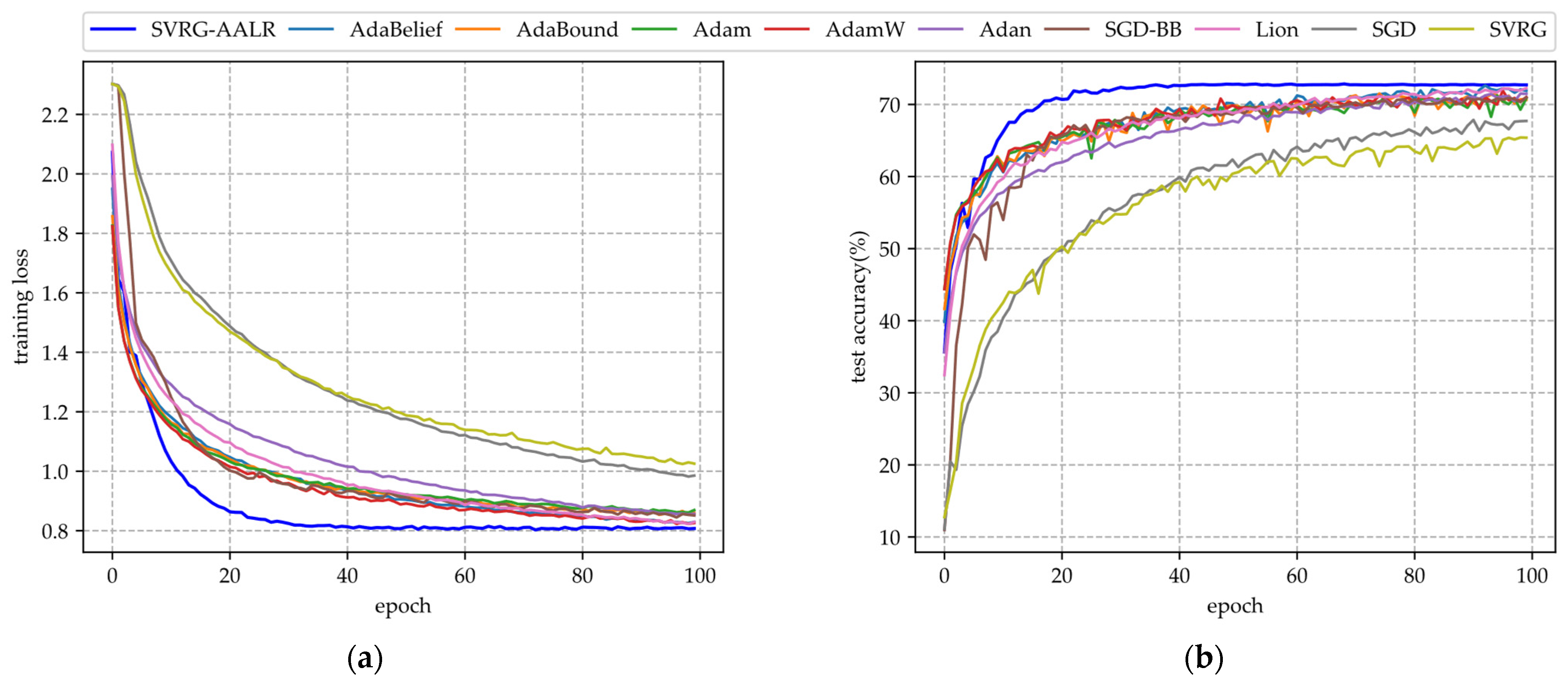
Figure 1 presents the training results on LeNet.

(i)

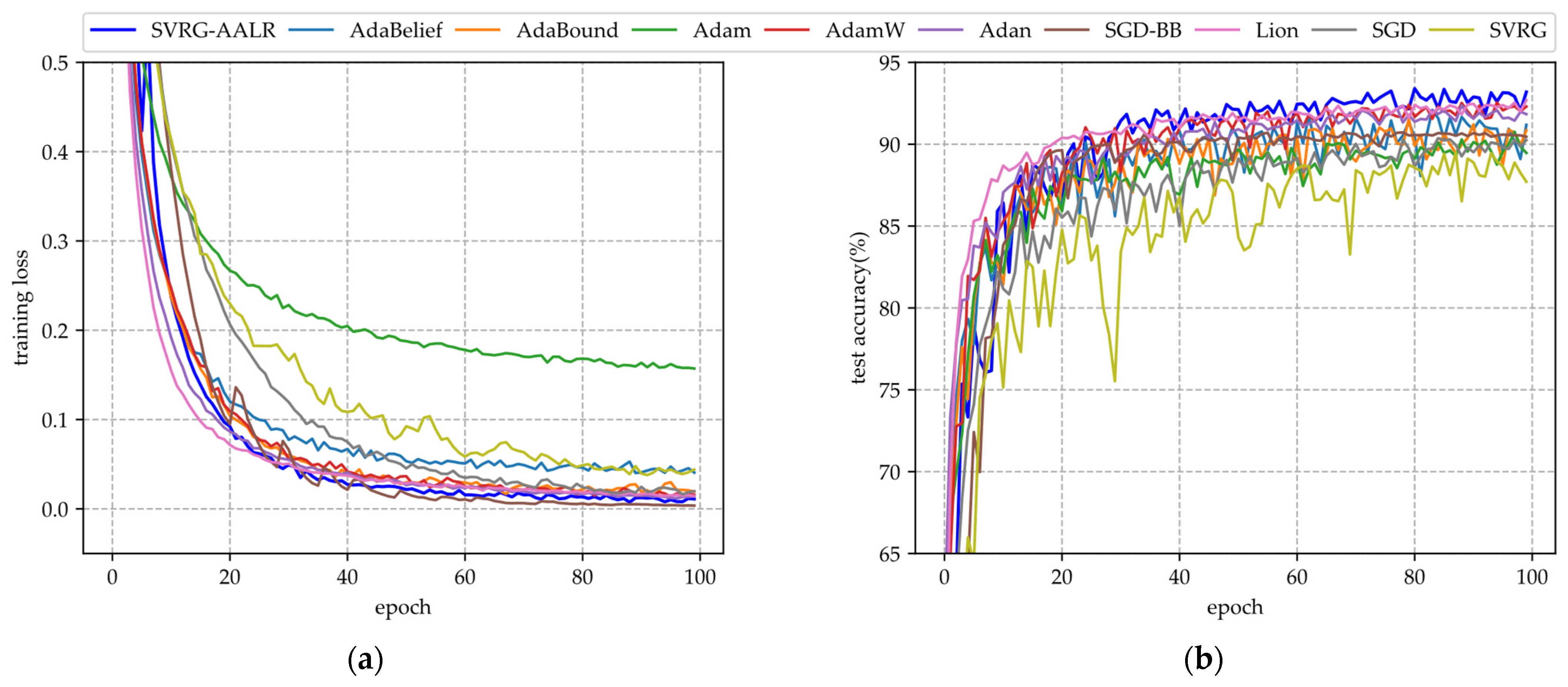
In Figure 1a, SVRG-AALR exhibits the fastest convergence rate, reaching approximately 0.8 by the 40th epoch. In contrast, Lion, AdamW, and AdaBelief only attain a similar level by the 100th epoch. Furthermore, the loss function values achieved by these four algorithms are significantly lower than those of other methods, highlighting their exceptional convergence performance. Conversely, SVRG and SGD demonstrate the poorest convergence outcomes, with SVRG performing even worse than SGD. Despite incorporating mini-batches into the SVRG framework during experimentation, its convergence performance remains unsatisfactory.

(ii)

In Figure 1b, the test accuracy of SVRG-AALR is observed to be the highest, with the curve beginning to stabilize in a flat region at the 40th iteration. In contrast, Lion, AdamW, and AdaBelief only approach the test accuracy achieved by SVRG-AALR at the 100th iteration. This finding indicates that SVRG-AALR possesses superior optimization capabilities and can identify more effective weights to enhance the test accuracy of the LeNet model. Furthermore, with the exception of SVRG-AALR, the test accuracy curves for other algorithms exhibit pronounced sawtooth patterns, suggesting that SVRG-AALR demonstrates greater stability compared to its counterparts. Given LeNet’s relatively simple deep model architecture and limited classification ability, it is noteworthy that all algorithms yield a test accuracy around 70%. In Figure 1, it is also evident that the overall performance of SVRG is slightly inferior to that of SGD.

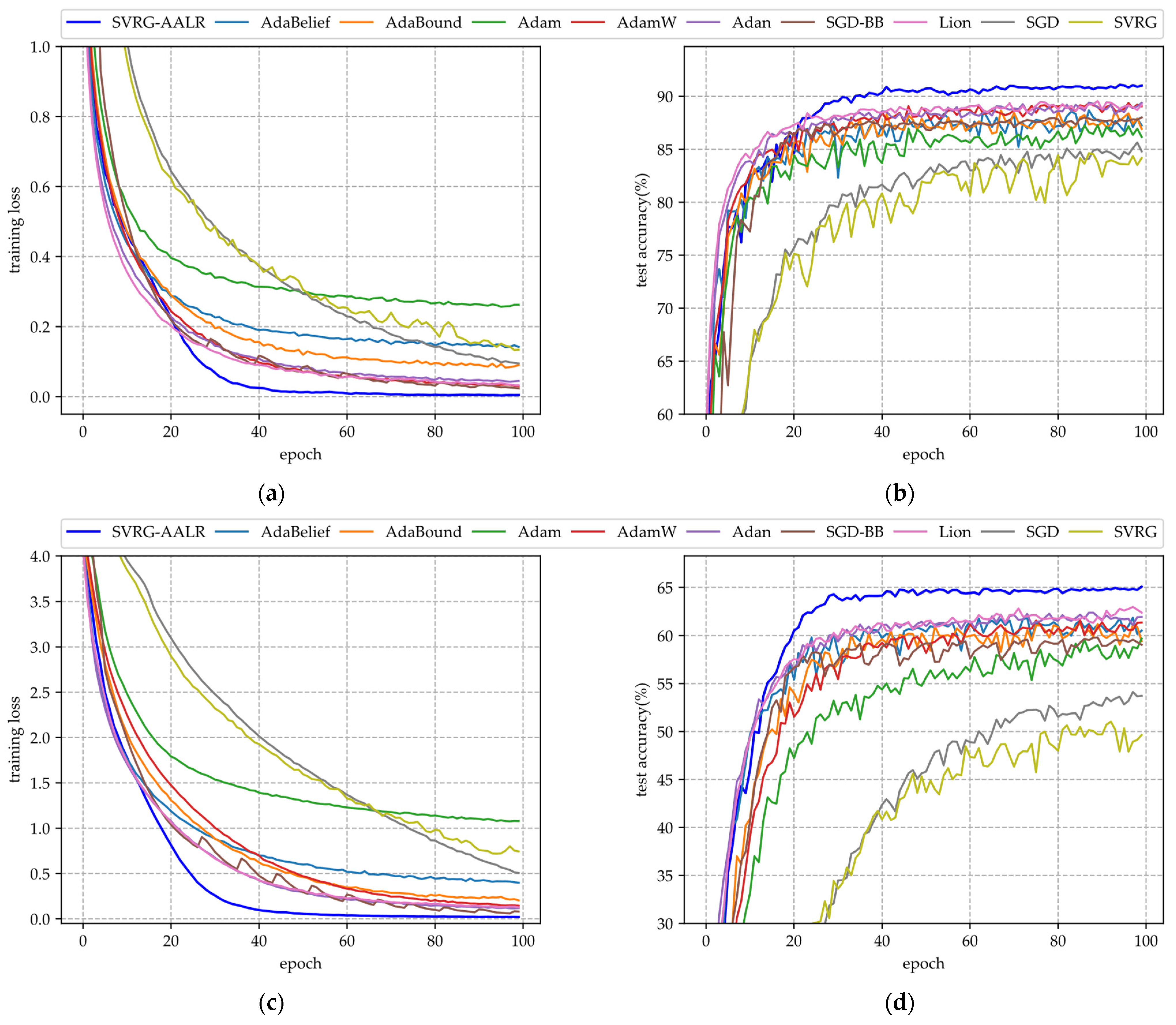
Figure 2 shows the training results on the VGG11 model.

(i)

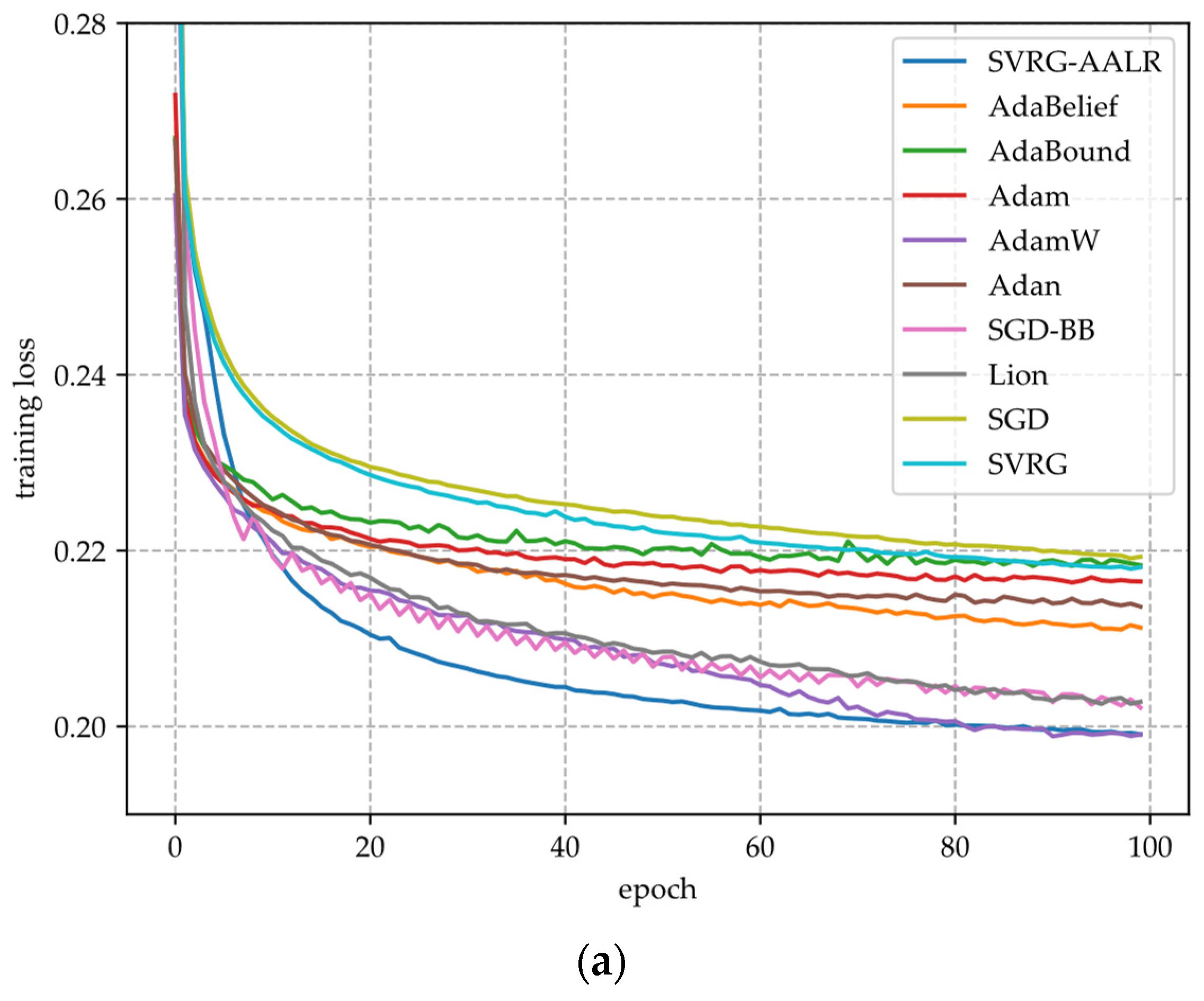
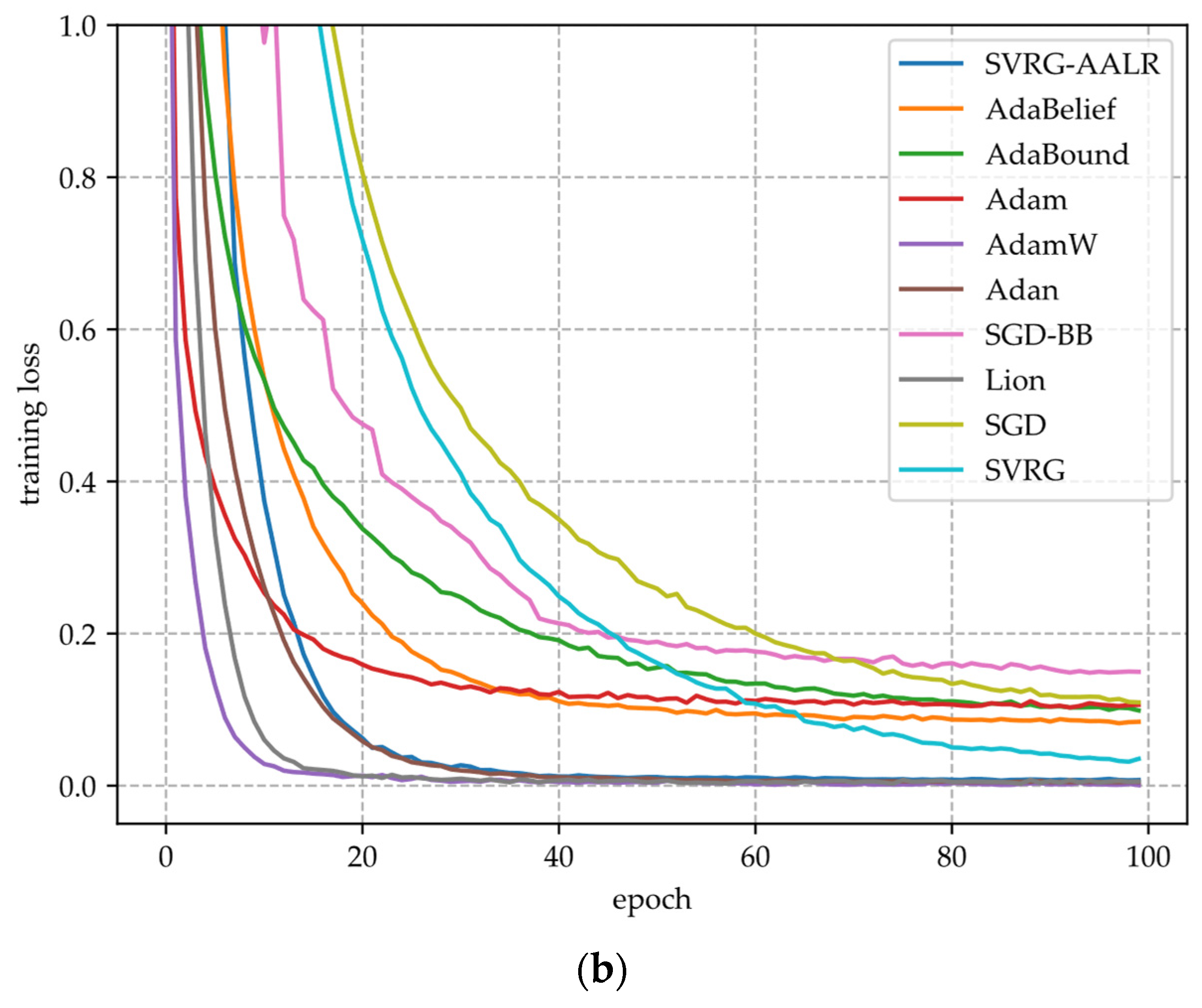
Figure 2a,c,e illustrate the training loss function curves of various algorithms applied to VGG11 across three datasets. From these figures, it is evident that SVRG-AALR achieves a final loss value approaching zero after 100 iterations. Both Lion and SGD-BB demonstrate convergence performance on CIFAR10 and CIFAR100 that closely aligns with SVRG-AALR; however, minor discrepancies remain. In contrast, Adam, SVRG, and SGD exhibit relatively poor performance across all three datasets. On the large-scale CINIC10 dataset, the loss function value for SVRG-AALR can also approach zero, while Lion, AdamW, and SGD-BB show deviations of approximately 10%. This finding indicates that SVRG-AALR maintains excellent convergence performance even on large-scale datasets. Furthermore, in all three datasets examined, the convergence curves for SVRG and SGD-BB display pronounced sawtooth patterns; conversely, those for SVRG-AALR are notably smoother. This suggests that SVRG-AALR possesses superior stability compared to its counterparts.

(ii)

Figure 2b,d,f illustrate the test accuracy curves of various algorithms across three datasets. From these figures, it is evident that SVRG-AALR achieves the highest accuracy, underscoring its superior optimization performance in identifying optimal weights to enhance the generalization capability of the VGG11 model, thereby resulting in elevated test accuracy. In all three figures, the test accuracy curves exhibit varying degrees of sawtooth patterns. This phenomenon can be attributed to the CIFAR100 dataset’s composition of 100 categories with relatively few training samples per category, which leads to significant fluctuations in model accuracy during training. Notably, SVRG-AALR displays the least pronounced sawtooth pattern among them; its test accuracy curve begins to stabilize around the 40th epoch of training. This outcome further illustrates the excellent iterative stability and convergence characteristics of SVRG-AALR and suggests that this proposed algorithm holds considerable potential for application in multi-classification scenarios with limited training data. The number of training samples for each category in CIFAR-100 is lower than that in CIFAR-10, resulting in a significantly reduced test accuracy as illustrated in Figure 2d compared to Figure 2b. At this juncture, the test accuracy achieved by SVRG-AALR is approximately 5% higher than that of Lion, indicating that the model trained using SVRG-AALR demonstrates commendable robustness and generalization capabilities even in scenarios with limited training data. In Figure 2f, both the smoothness of the SVRG-AALR curve and its corresponding test accuracy are superior to those of all other algorithms. Furthermore, it is noteworthy that the test accuracy curve begins to stabilize when the algorithm reaches the 40th epoch. This observation suggests that SVRG-AALR can attain a high level of accuracy with fewer training iterations on large-scale datasets, highlighting its potential competitiveness in extensive applications. In Figure 2, the overall performance of SVRG is worse than SGD, while the overall performance of SVRG-AALR is better than Lion.

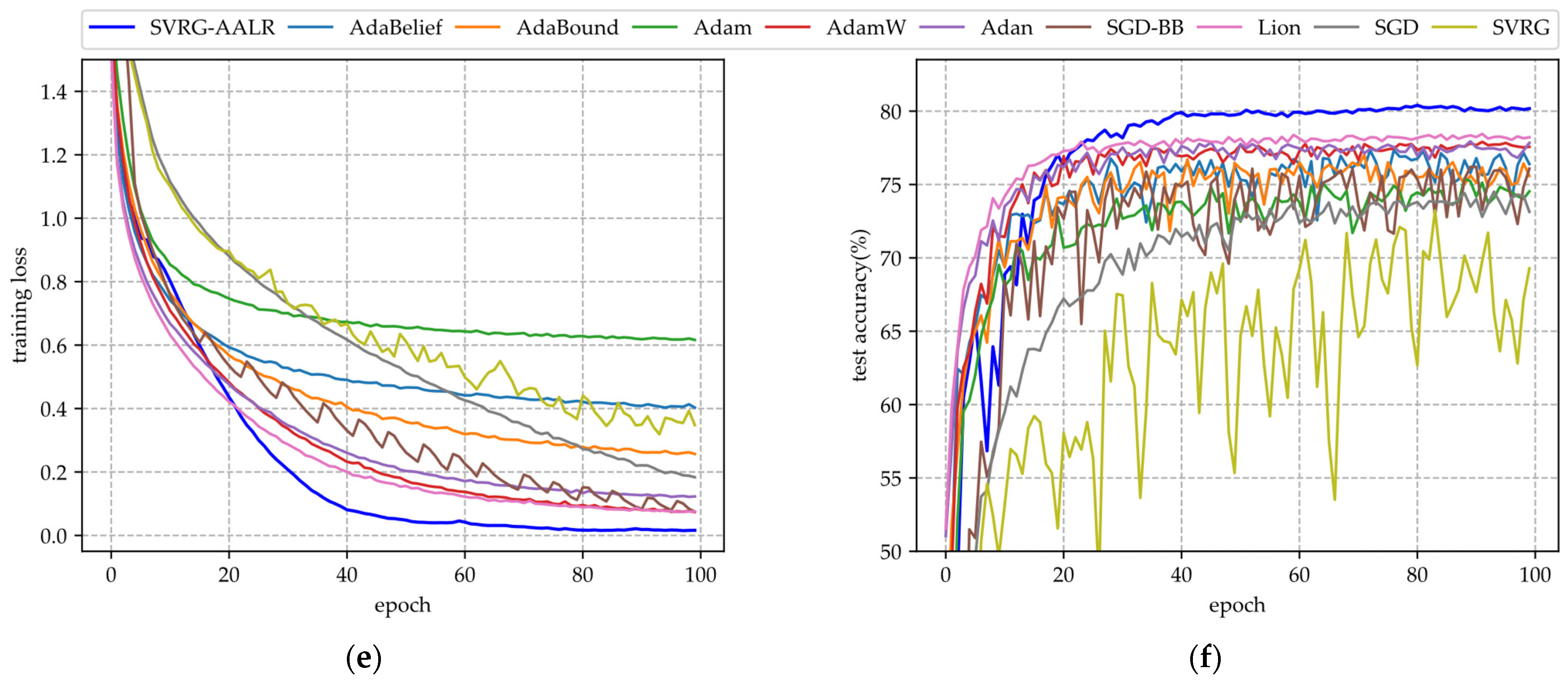
Figure 3 shows the training results on ResNet34.

(i)

Figure 3a,c,e illustrate the training loss function curves of various algorithms across three datasets. From these figures, it is evident that the convergence curve of SVRG-AALR begins to enter a flat region at the 40th iteration and approaches zero, exhibiting a generally smooth trajectory. This behavior indicates that this algorithm possesses characteristics of rapid convergence and stable iterations. In contrast, the loss function values for Lion, AdamW, and SGD-BB only converge towards those of SVRG-AALR by the 100th iteration, suggesting that their convergence speeds are slower than that of SVRG-AALR. Additionally, the three curves corresponding to SGD-BB display more pronounced sawtooth patterns, reflecting its instability during iterations. Overall, across all three datasets, it can be concluded that the convergence performance of SVRG remains inferior to that of SGD.

(ii)

The test accuracy curves of various algorithms for the three datasets are presented in Figure 3b,d,f. From these figures, it is evident that the test accuracy curves of all algorithms exhibit varying degrees of sawtooth patterns, with those of SGD-BB, SVRG, and Adam being particularly pronounced. Notably, while the training loss function of SGD-BB converges to zero after 100 iterations, its corresponding test accuracy curve displays the most significant sawtooth pattern along with a relatively low overall accuracy. This observation indicates potential overfitting during training. Overall, SVRG-AALR achieves the highest accuracy among the tested algorithms. Its test accuracy curve begins to stabilize after approximately 40 iterations and exhibits the smallest amplitude in its sawtooth pattern. This suggests that SVRG-AALR possesses strong anti-overfitting capabilities and that the trained ResNet34 model demonstrates good generalization performance. The test accuracy curve for Lion ranks second overall; however, when compared to SVRG-AALR, there exists an average gap of about 5% in their respective accuracies. This finding implies that SVRG-AALR outperforms Lion in terms of optimization performance. In Figure 3, it is also observed that SVRG performs worse than SGD.

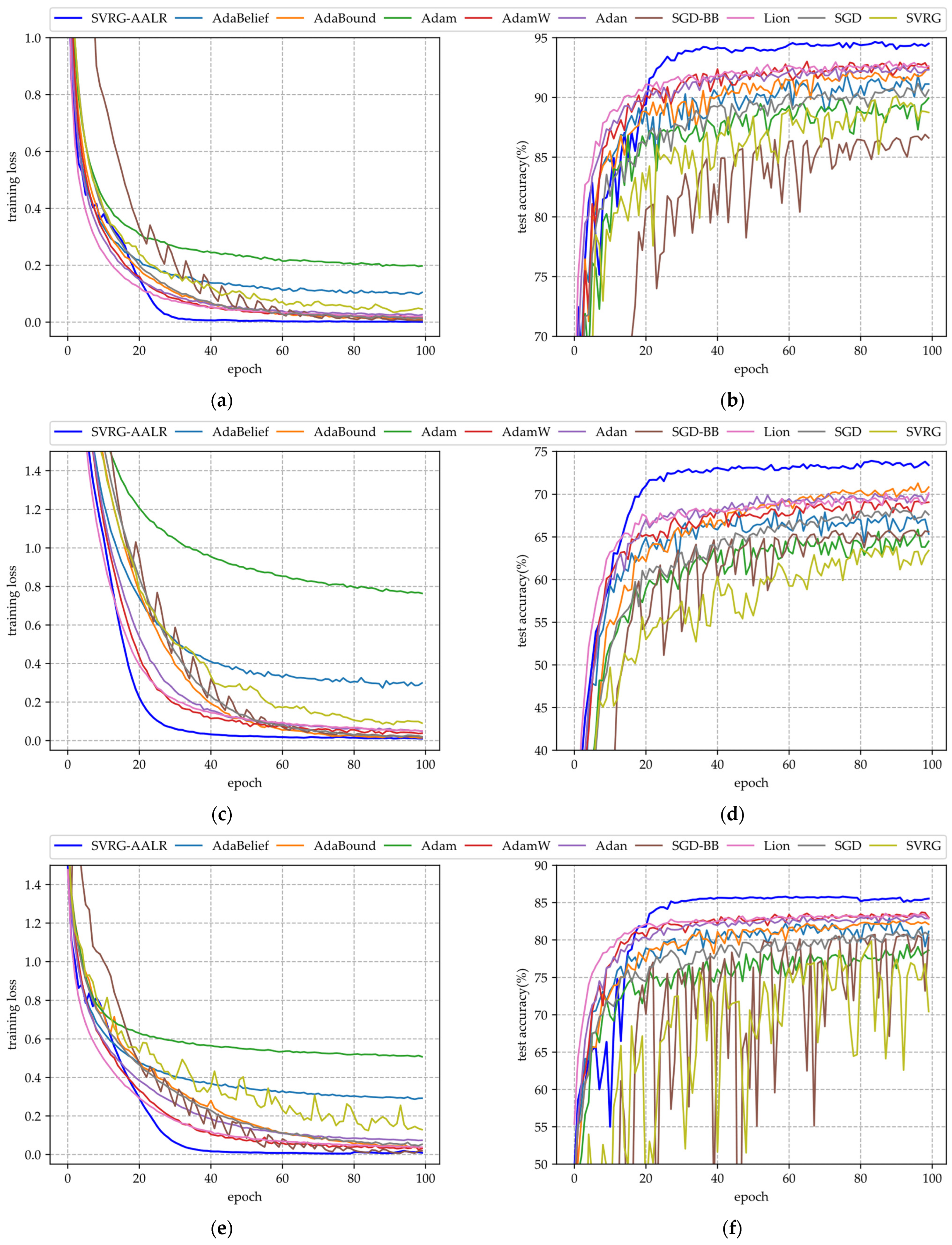
Figure 4 reveals the training results on DenseNet.

(i)

Figure 4a,c illustrate the training loss function curves for each algorithm across two datasets. From these curves, it is evident that SVRG-AALR and SGD-BB exhibit superior convergence, approaching a loss of zero after 100 iterations, thereby demonstrating excellent performance in terms of convergence. In comparison to Figure 2a,c and Figure 3a,c, the sawtooth phenomenon observed in Figure 4a,c is more pronounced. This phenomenon can be attributed to the structural characteristics inherent in the DenseNet model. To mitigate the parameter scale of the model, DenseNet employs dense connections and feature reuse techniques within its architecture. However, this dense connectivity introduces significant parameter coupling issues; specifically, each layer’s output in DenseNet is concatenated with feature maps from all preceding layers along the channel dimension. Consequently, there exists a high degree of parameter interdependence among layers. Adjusting any single layer may disrupt the global feature propagation path, complicating weight adjustments throughout the model. This challenge manifests as an increased number of sawteeth in the convergence curve.

(ii)

Figure 4b,d illustrate the test accuracy curves of various algorithms across two datasets. In comparison to Figure 3b,d, the sawtooth patterns present in each curve are significantly diminished, indicating that DenseNet, which utilizes dense connections and feature reuse techniques, exhibits a superior capability for mitigating overfitting when compared to ResNet. However, it is noteworthy that SVRG-AALR still achieves the highest accuracy in Figure 4b,d; nonetheless, its accuracy is slightly lower than before, with more pronounced sawtooth patterns relative to the corresponding curves in Figure 3b,d. This observation further suggests that weight adjustment within DenseNet poses greater challenges. Nevertheless, it is evident from Figure 4b,d that SVRG-AALR continues to outperform other baseline algorithms regarding accuracy. This finding demonstrates that SVRG-AALR maintains strong performance on DNN models where weight adjustment proves difficult. In Figure 4, while the overall performance of SVRG remains inferior to that of SGD, it is observed that SVRG-AALR performs slightly better than Lion overall.

Appendix A presents the confusion matrix plots for ResNet34 applied to the CIFAR10 and CINIC10 datasets. Figure A1 illustrates the results on the CIFAR10 dataset, where the maximum misclassification rate for any single category is approximately 1%, indicating a relatively high level of accuracy. In contrast, Figure A2 displays the outcomes on the CINIC10 dataset, revealing that around 10% of samples in the automobile category are misclassified as trucks, and vice versa. Similarly, about 10% of samples in the cat category are incorrectly classified as dogs, and vice versa. These elevated misclassification rates can primarily be attributed to downsampling of the original ImageNet images, which leads to image distortion. Overall, the two confusion matrix plots presented in Appendix A demonstrate that ResNet34 trained using SVRG-AALR achieves high accuracy across large-scale multi-category image datasets, suggesting that SVRG-AALR is well-suited for training DNN models.

Table 2. The classification results of ResNet34 trained by each optimizer on the test set.

(a) CIFAR10 dataset
Optimizer	Acc	Prec	Recall	F1
AdaBelief	0.9204	0.9222	0.9204	0.9207
AdaBound	0.9254	0.9252	0.9254	0.9250
Adam	0.8995	0.8999	0.8995	0.8990
AdamW	0.9301	0.9305	0.9301	0.9301
Adan	0.9267	0.9268	0.9267	0.9266
SGD-BB	0.8689	0.8690	0.8689	0.8688
Lion	0.9303	0.9304	0.9303	0.9303
SVRG	0.9012	0.9028	0.9012	0.9015
SGD	0.9116	0.9116	0.9116	0.9115
SVRG-AALR	0.9465	0.9465	0.9465	0.9464
(b) CIFAR100 dataset
Optimizer	Acc	Prec	Recall	F1
AdaBelief	0.6824	0.7000	0.6824	0.6815
AdaBound	0.7127	0.7176	0.7127	0.7133
Adam	0.6587	0.6813	0.6587	0.6584
AdamW	0.6926	0.7020	0.6926	0.6929
Adan	0.7009	0.7105	0.7009	0.7014
SGD-BB	0.6576	0.6604	0.6576	0.6577
Lion	0.7016	0.7061	0.7016	0.7006
SVRG	0.6392	0.6594	0.6392	0.6407
SGD	0.6844	0.6894	0.6844	0.6840
SVRG-AALR	0.7389	0.7405	0.7389	0.7383
(c) CINIC10 dataset
Optimizer	Acc	Prec	Recall	F1
AdaBelief	0.8292	0.8296	0.8292	0.8289
AdaBound	0.8264	0.8275	0.8264	0.8259
Adam	0.7937	0.7963	0.7937	0.7933
AdamW	0.8370	0.8366	0.8370	0.8364
Adan	0.8325	0.8345	0.8325	0.8230
SGD-BB	0.8071	0.8077	0.8071	0.8073
Lion	0.8355	0.8353	0.8355	0.8351
SVRG	0.7985	0.8008	0.7985	0.7977
SGD	0.8129	0.8147	0.8129	0.8135
SVRG-AALR	0.8587	0.8584	0.8587	0.8585

presents the classification results of ResNet34 trained by various optimizers on the test set.

(i)

On the CIFAR10 dataset, the model trained using SVRG-AALR achieved an F1 score of 0.9464, securing the top position among all optimizers. In comparison, the model trained with the Lion optimizer attained an F1 score of 0.9303, placing it in second position. Overall, on the CIFAR10 dataset, SVRG-AALR demonstrates a marginally superior performance compared to Lion.

(ii)

On the CIFAR100 dataset, the model trained using SVRG-AALR achieved an F1 score of 0.7383, securing the top position among all optimizers. In comparison, the model trained with the AdaBound optimizer attained an F1 score of 0.7133, placing it in second position. Overall, the performance of SVRG-AALR on the CIFAR100 dataset demonstrates a slight advantage over that of AdaBound.

(iii)

On the CINIC10 dataset, the model trained using SVRG-AALR achieved an F1 score of 0.8585, securing the top position among all optimizers. In comparison, the model trained with the AdamW optimizer attained an F1 score of 0.8364, placing it in second position. Overall, on the CINIC10 dataset, SVRG-AALR demonstrates a marginally superior performance compared to AdamW.

Based on the analysis of the data presented in Table 2, it is evident that the performance of SVRG-AALR is comparable to, and in some cases even superior to, that of advanced optimizers such as AdamW, AdaBound, and Lion utilized in recent years. Consequently, SVRG-AALR demonstrates both effectiveness and advancement for training DNN models.

Table 3. Comparison of the average computation time per epoch for each algorithm on the CIFAR-10 dataset.

Algorithm	Computation Time/s
	LeNet	VGG11	ResNet34	DenseNet121
SVRG-AALR	16.6	29.6	159.8	331.1
AdaBelief	10.1	17.3	64.3	138.1
AdaBound	9.5	17.5	63.3	135.8
Adam	9.1	17.8	58.9	115.3
AdamW	9.5	16.2	60.1	115.5
Adan	10.3	23.5	68.5	149.7
SGD-BB	8.7	15.3	60.6	123.9
Lion	8.9	16.9	60.4	130.5
SGD	8.6	15.1	57.7	114.9
SVRG	19.1	32.9	172.8	361.3

presents the average computing time (in seconds) for each algorithm over one epoch on the CIFAR-10 dataset. As illustrated in Table 3, the computing time of SVRG-AALR is comparable to that of traditional SVRG, with both significantly exceeding the computation times of other algorithms. The primary reason for this discrepancy is that SVRG requires additional time to compute the full gradient across all samples.

Figure 5 illustrates the dynamic curves of the AALR for the VGG11 and ResNet34 models during training on the CIFAR-10 dataset, with an initial learning rate set at 0.01. As depicted in Figure 5, both learning rate curves exhibit a rapid increase during the first ten iterations, followed by a gradual decline that brings them below 0.01, where they stabilize relatively. Figure 2a and Figure 3a demonstrate that the training loss functions for both the VGG11 and ResNet34 models decrease sharply within the initial ten iterations before entering a more stable phase. Notably, during these early iterations, both AALR learning rate curves maintain a state of fluctuation without exhibiting prolonged periods of constancy (i.e., no change). This observation indicates that the AALR learning rate is capable of adapting to variations in parameters and gradients effectively. Furthermore, as illustrated in Figure 5, the AALR learning rates on both curves exceed 0.05 during the early iterations and maintain a certain distance from zero in the later iterations. This observation suggests that the AALR learning rate rarely activates the overly conservative revision strategies outlined in Equations (16) and (17) throughout the iteration process. In this experiment, with ${\phi }_0=0.00002$, it follows from Equations (16) and (17) that if the AALR learning rate were to trigger these overly conservative revision strategies, we would expect to see both learning rate curves in Figure 5 approaching zero. Simultaneously, no instances of a learning rate exceeding 1—indicative of an excessively high learning rate—are observed in Figure 5. Therefore, it can be concluded that the sensitivity of the AALR learning rate to the threshold revision strategies described by Equations (16) and (17) is contingent upon the value of ${\phi }_0$. When ${\phi }_0$ is small, there exists a low probability for the AALR learning rate to activate these threshold revision strategies; consequently, under such conditions, it exhibits reduced sensitivity towards them. Conversely, when ${\phi }_0$ is large, there is an increased likelihood for triggering these threshold revisions; thus, at this point, the AALR learning rate becomes more sensitive to such strategies. Moreover, Figure 5 further indicates that adopting a smaller value for ${\phi }_0$ proves more advantageous—for instance, using ${\phi }_0=0.00002$ as proposed in this paper allows for optimal adaptability of the AALR learning rate to variations in parameters and gradients while minimizing excessive intervention through revisions. Based on the analysis of Figure 5 above, it is evident that the AALR demonstrates excellent adaptability. In the initial stages of iteration, it can automatically increase to expedite the convergence of DNN training. Conversely, in the later stages of iteration, it decreases and stabilizes at a small value to prevent divergence during DNN training. Furthermore, the magnitude of the learning rate is effectively maintained within a reasonable range. Overall, Figure 5 illustrates that both the calculation method for AALR and its application within SVRG are effective.

Figure 6 illustrates the training loss function curves of VGG11 applied to two non-computer vision datasets. The bank marketing dataset pertains to direct marketing campaigns (phone calls) conducted by a Portuguese banking institution, with the objective of predicting whether clients will subscribe to a term deposit [49]. The 20 Newsgroups dataset is a multi-class text classification resource that encompasses 20 major categories and approximately 20,000 documents in total [50]. As depicted in Figure 6, the training loss function for SVRG-AALR consistently decreases across both datasets.

Table 4. The classification metric values of the models trained by each algorithm on two non-computer vision datasets.

(a) Bank marketing dataset
Optimizer	Acc	Prec	Recall	F1
SVRG-AALR	0.9009	0.7789	0.6953	0.7266
AdaBelief	0.9020	0.7857	0.6900	0.7242
AdaBound	0.9014	0.7879	0.6782	0.7149
Adam	0.9014	0.7910	0.6723	0.7104
AdamW	0.9011	0.7816	0.6903	0.7234
Adan	0.9005	0.7810	0.6844	0.7185
SGD-BB	0.9011	0.7833	0.6860	0.7203
Lion	0.9024	0.7868	0.6910	0.7253
SGD	0.9010	0.7863	0.6780	0.7144
SVRG	0.8998	0.7834	0.6714	0.7080
(b) 20 Newsgroups dataset
Optimizer	Acc	Prec	Recall	F1
SVRG-AALR	0.8480	0.8471	0.8454	0.8457
AdaBelief	0.8403	0.8403	0.8375	0.8381
AdaBound	0.8347	0.8363	0.8315	0.8329
Adam	0.8469	0.8465	0.8445	0.8447
AdamW	0.8414	0.8398	0.8373	0.838
Adan	0.8321	0.8315	0.8287	0.8295
SGD-BB	0.8241	0.8255	0.8201	0.8213
Lion	0.8475	0.8481	0.8458	0.8457
SGD	0.8204	0.8206	0.8176	0.8184
SVRG	0.8294	0.8302	0.8265	0.8276

presents the classification metric values achieved on these two non-computer vision datasets. It is evident from Table 4 that the F1 scores for models trained using SVRG-AALR on the bank marketing and 20 Newsgroups datasets are recorded at 0.7266 and 0.8457, respectively, indicating a relatively high level of accuracy maintained throughout. The experimental results illustrated in Figure 6 and detailed in Table 4 further confirm that the SVRG-AALR algorithm remains effective when applied to non-computer vision datasets, thereby demonstrating its broad applicability across various domains.

Based on the experimental analysis presented above, it can be concluded that when employing SVRG-AALR for training DNN models, the following characteristics are observed:

(i)

The training process demonstrates convergence, with a relatively rapid convergence speed. The experimental results presented above indicate that the training trajectory of SVRG-AALR across various DNN models and datasets exhibits a favorable convergence trend, aligning with the conclusions drawn from the convergence analysis of the SVRG-AALR algorithm. Furthermore, the number of iterations required for both the training loss function curve and the test accuracy curve of SVRG-AALR to stabilize in a flat region is lower than that observed with baseline optimizers; thus, this algorithm showcases a comparatively swift convergence rate. As illustrated in line 13 of Algorithm 2, the update formula for adjusting DNN weights is

$$w_{k,t+1}=w_{k,t}-{\tilde{\alpha }}_k{\upsilon }_{k,t}$$

(53)

where the learning rate ${\tilde{\alpha }}_k$ is derived from the quasi-Newton method as outlined in Equations (5) and (6). Consequently, ${\tilde{\alpha }}_k$ incorporates second-order information and is adjusted to prevent it from being excessively large or small, thereby facilitating the acceleration of convergence for the SVRG-AALR algorithm.

(ii)

The trained DNN model demonstrates a high level of classification accuracy. The weight parameters are critical factors that influence the classification performance of the DNN model; thus, elevated classification accuracy reflects superior quality of these weights. In Algorithm 2, ${\upsilon }_{k,t}$ represents the gradient adjusted through mini-batch and variance reduction techniques, resulting in relatively low gradient variance for ${\upsilon }_{k,t}$. As indicated in Equation (53), the adaptive AALR learning rate ${\tilde{\alpha }}_k$ is capable of adapting to ${\upsilon }_{k,t}$, which enhances the precision of the weight update term $∆w_{k,t}=-{\tilde{\alpha }}_k{\upsilon }_{k,t}$. This feature not only accelerates convergence for SVRG-AALR but also improves weight quality, ultimately leading to enhanced classification accuracy for the trained DNN model.

(iii)

The training process exhibits commendable stability. The accuracy of $∆w_{k,t}$ allows SVRG-AALR to maintain a high level of stability throughout the iterative process. This stability is evident in both the training loss function curve and the test accuracy curve, which display relatively smooth trajectories with fewer sawtooth patterns.

The experimental results and analyses presented above demonstrate that the adaptive AALR and other strategies proposed in this paper can effectively extend the stochastic variance-reduced gradient (SVRG) theory to the domain of deep neural network (DNN) training. The SVRG-AALR algorithm exhibits strong convergence during training, and the resulting DNN model showcases excellent generalization capabilities. Consequently, the SVRG-AALR algorithm proves to be an effective approach for DNN training.

5. Conclusions

The theoretical advantages of SVRG render it particularly well-suited for addressing the gradient variance issue encountered in DNN training. However, the algorithm faces adaptation challenges that significantly diminish its effectiveness when applied directly to DNN training scenarios. To address this limitation, this paper proposes a comprehensive set of strategies aimed at extending SVRG. The outer loop of SVRG primarily focuses on computing the full gradient and determining the learning rate. The computation of the full gradient aligns with traditional SVRG practices, while the calculation of the learning rate represents a novel contribution tailored for DNN training. The formula for calculating the learning rate is derived using both quasi-Newton methods and Barzilai–Borwein techniques, thereby incorporating second-order information into the process. By employing an alternating strategy that utilizes two distinct formulas for learning rate calculation, we ensure that both parameter change rates and gradient change rates are integrated into the weight update process with equal probability. Furthermore, the mini-batch average gradients computed in each iteration of the inner loop are aggregated into a gradient with reduced variance following inertial correction. This refined gradient is then relayed back to the outer loop for the calculation of the new learning rate. Experimental results obtained from the LeNet, VGG11, ResNet34, and DenseNet121 models demonstrate that the SVRG-AALR algorithm exhibits exceptional training convergence and robust generalization capabilities across DNN models with varying characteristics and scales. Overall, its training performance is comparable to or even surpasses that of advanced optimizers such as AdamW, AdaBound, and Lion. Thus, it can be concluded that the adaptation strategy and methodology proposed in this paper effectively extend SVRG theory to DNN model training scenarios while remaining competitive.

Although this paper has achieved the aforementioned results, certain deficiencies remain. (i) The effectiveness of SVRG-AALR in other domains of DNNs warrants further investigation. For example, it is yet to be determined whether SVRG-AALR can yield superior outcomes in large-scale DNN applications such as medical image recognition and power system load forecasting. (ii) There exists potential for enhancement in the gradient acceleration capabilities of SVRG-AALR. Numerous successful gradient acceleration techniques found in advanced optimizers like AdamW, AdaBound, and Lion possess both theoretical significance and practical applicability when adapted to SVRG-AALR. Furthermore, many implementation details require additional exploration in practice. (iii) The SVRG-AALR algorithm computes the full gradient across all training samples, which significantly increases its computational time and hinders its applicability in large-scale training datasets. Therefore, future research should prioritize the exploration of methods for calculating the full gradient that incur lower computational costs, as this represents an urgent challenge that needs to be addressed.

References

1. Chai, J.; Zeng, H.; Li, A.; Ngai, E.W. Deep learning in computer vision: A critical review of emerging techniques and application scenarios. Mach. Learn. Appl. 2021, 6, 100134. [Google Scholar] [CrossRef]
2. Otter, D.W.; Medina, J.R.; Kalita, J.K. A survey of the usages of deep learning for natural language processing. IEEE Trans. Neural Netw. Learn. Syst. 2020, 32, 604–624. [Google Scholar] [CrossRef]
3. Shamshirband, S.; Fathi, M.; Dehzangi, A.; Chronopoulos, A.T.; Alinejad-Rokny, H. A review on deep learning approaches in healthcare systems: Taxonomies, challenges, and open issues. J. Biomed. Inform. 2021, 113, 103627. [Google Scholar] [CrossRef]
4. Khallaf, R.; Khallaf, M. Classification and analysis of deep learning applications in construction: A systematic literature review. Autom. Constr. 2021, 129, 103760. [Google Scholar] [CrossRef]
5. Li, C.; Zhang, S.; Qin, Y.; Estupinan, E. A systematic review of deep transfer learning for machinery fault diagnosis. Neurocomputing 2020, 407, 121–135. [Google Scholar] [CrossRef]
6. Altalak, M.; Ammad uddin, M.; Alajmi, A.; Rizg, A. Smart agriculture applications using deep learning technologies: A survey. Appl. Sci. 2022, 12, 5919. [Google Scholar] [CrossRef]
7. Khodayar, M.; Regan, J. Deep neural networks in power systems: A review. Energies 2023, 16, 4773. [Google Scholar] [CrossRef]
8. Roux, N.; Schmidt, M.; Bach, F. A stochastic gradient method with an exponential convergence rate for finite training sets. In Proceedings of the 26th Annual Conference on Neural Information Processing Systems (2012), Lake Tahoe, NV, USA, 3–6 December 2012. [Google Scholar]
9. Johnson, R.; Zhang, T. Accelerating stochastic gradient descent using predictive variance reduction. In Proceedings of the NIPS 2013, Stateline, NV, USA, 5–10 December 2013. [Google Scholar]
10. Shang, F.; Zhou, K.; Liu, H.; Cheng, J.; Tsang, I.W.; Zhang, L.; Tao, D.; Jiao, L. VR-SGD: A simple stochastic variance reduction method for machine learning. IEEE Trans. Knowl. Data Eng. 2018, 32, 188–202. [Google Scholar] [CrossRef]
11. Alioscha-Perez, M.; Oveneke, M.C.; Sahli, H. SVRG-MKL: A fast and scalable multiple kernel learning solution for features combination in multi-class classification problems. IEEE Trans. Neural Netw. Learn. Syst. 2019, 31, 1710–1723. [Google Scholar] [CrossRef] [PubMed]
12. Tankaria, H.; Yamashita, N. A stochastic variance reduced gradient using Barzilai-Borwein techniques as second order information. J. Ind. Manag. Optim. 2024, 20, 525–547. [Google Scholar] [CrossRef]
13. Fu, S.; Wang, X.; Tang, J.; Lan, S.; Tian, Y. Generalized robust loss functions for machine learning. Neural Netw. 2024, 171, 200–214. [Google Scholar] [CrossRef] [PubMed]
14. Defazio, A.; Bottou, L. On the ineffectiveness of variance reduced optimization for deep learning. In Proceedings of the 2019 Conference on Neural Information Processing Systems, Vancouver, BC, Canada, 8–14 December 2019. [Google Scholar]
15. Shi, L.; Zhao, H.; Zakharov, Y. Generalized variable step size continuous mixed p-norm adaptive filtering algorithm. IEEE Trans. Circuits Syst. II Express Briefs 2019, 66, 1078–1082. [Google Scholar] [CrossRef]
16. Shi, L.; Zhao, H.; Zeng, X.; Yu, Y. Variable step-size widely linear complex-valued NLMS algorithm and its performance analysis. Signal Process. 2019, 165, 1–6. [Google Scholar] [CrossRef]
17. Shi, L.; Zhao, H.; Zakharov, Y.; Chen, B.; Yang, Y. Variable step-size widely linear complex-valued affine projection algorithm and performance analysis. IEEE Trans. Signal Process. 2020, 68, 5940–5953. [Google Scholar] [CrossRef]
18. Tan, C.; Ma, S.; Dai, Y.-H.; Qian, Y. Barzilai-Borwein step size for stochastic gradient descent. In Proceedings of the 2016 Conference on Neural Information Processing Systems, Barcelona, Spain, 5–10 December 2016. [Google Scholar]
19. Yu, T.; Liu, X.-W.; Dai, Y.-H.; Sun, J. Stochastic variance reduced gradient methods using a trust-region-like scheme. J. Sci. Comput. 2021, 87, 5. [Google Scholar] [CrossRef]
20. Li, J.; Xue, D.; Liu, L.; Qi, R. A stochastic variance reduced gradient method with adaptive step for stochastic optimization. Optim. Control Appl. Methods 2024, 45, 1327–1342. [Google Scholar] [CrossRef]
21. Barzilai, J.; Borwein, J.M. Two-point step size gradient methods. IMA J. Numer. Anal. 1988, 8, 141–148. [Google Scholar] [CrossRef]
22. Yu, L.; Deng, T.; Zhang, W.; Zeng, Z. Stronger adversarial attack: Using mini-batch gradient. In Proceedings of the 2020 12th International Conference on Advanced Computational Intelligence (ICACI), Dali, China, 14–16 August 2020; pp. 364–370. [Google Scholar]
23. Smirnov, E.; Oleinik, A.; Lavrentev, A.; Shulga, E.; Galyuk, V.; Garaev, N.; Zakuanova, M.; Melnikov, A. Face representation learning using composite mini-batches. In Proceedings of the IEEE/CVF International Conference on Computer Vision Workshops, Seoul, Republic of Korea, 27–28 October 2019; pp. 551–559. [Google Scholar]
24. Peng, C.; Xiao, T.; Li, Z.; Jiang, Y.; Zhang, X.; Jia, K.; Yu, G.; Sun, J. Megdet: A large mini-batch object detector. In Proceedings of the IEEE Conference on Computer Vision and Pattern Recognition, Salt Lake City, UT, USA, 18–23 June 2018; pp. 6181–6189. [Google Scholar]
25. Yang, Z.; Wang, C.; Zhang, Z.; Li, J. Mini-batch algorithms with online step size. Knowl.-Based Syst. 2019, 165, 228–240. [Google Scholar] [CrossRef]
26. Li, M.; Zhang, T.; Chen, Y.; Smola, A.J. Efficient mini-batch training for stochastic optimization. In Proceedings of the 20th ACM SIGKDD International Conference on Knowledge Discovery and Data Mining, New York, NY, USA, 24–27 August 2014; pp. 661–670. [Google Scholar]
27. Chen, C.; Shen, L.; Zou, F.; Liu, W. Towards practical adam: Non-convexity, convergence theory, and mini-batch acceleration. J. Mach. Learn. Res. 2022, 23, 1–47. [Google Scholar]
28. Dokuz, Y.; Tufekci, Z. Mini-batch sample selection strategies for deep learning based speech recognition. Appl. Acoust. 2021, 171, 107573. [Google Scholar] [CrossRef]
29. Yin, Y.; Xu, Z.; Li, Z.; Darrell, T.; Liu, Z. A Coefficient Makes SVRG Effective. The Thirteenth International Conference on Learning Representations. arXiv 2025, arXiv:2311.05589. [Google Scholar]
30. Dai, Y.-H.; Huang, Y.; Liu, X.-W. A family of spectral gradient methods for optimization. Comput. Optim. Appl. 2019, 74, 43–65. [Google Scholar] [CrossRef]
31. Burdakov, O.; Dai, Y.; Huang, N. Stabilized barzilai-borwein method. J. Comput. Math. 2019, 37, 916–936. [Google Scholar] [CrossRef]
32. Liang, J.; Xu, Y.; Bao, C.; Quan, Y.; Ji, H. Barzilai–Borwein-based adaptive learning rate for deep learning. Pattern Recognit. Lett. 2019, 128, 197–203. [Google Scholar] [CrossRef]
33. Krizhevsky, A.; Hinton, G. Learning Multiple Layers of Features from Tiny Images. 2009. Available online: http://www.cs.utoronto.ca/~kriz/learning-features-2009-TR.pdf (accessed on 23 July 2025).
34. Darlow, L.N.; Crowley, E.J.; Antoniou, A.; Storkey, A.J. CINIC-10 Is Not ImageNet or CIFAR-10. University of Edinburgh. arXiv 2018, arXiv:1810.03505. [Google Scholar]
35. Chrabaszcz, P.; Loshchilov, I.; Hutter, F. A downsampled variant of imagenet as an alternative to the cifar datasets. arXiv 2017, arXiv:1707.08819. [Google Scholar] [CrossRef]
36. Deng, J.; Dong, W.; Socher, R.; Li, L.-J.; Li, K.; Fei-Fei, L. Imagenet: A large-scale hierarchical image database. In Proceedings of the 2009 IEEE Conference on Computer Vision and Pattern Recognition, Miami, FL, USA, 20–25 June 2009; pp. 248–255. [Google Scholar]
37. Lecun, Y.; Bottou, L.; Bengio, Y.; Haffner, P. Gradient-based learning applied to document recognition. Proc. IEEE 1998, 86, 2278–2324. [Google Scholar] [CrossRef]
38. Simonyan, K.; Zisserman, A. Very deep convolutional networks for large-scale image recognition. International Conference on Learning Representations. arXiv 2014, arXiv:1409.1556. [Google Scholar]
39. He, K.; Zhang, X.; Ren, S.; Sun, J. Deep residual learning for image recognition. In Proceedings of the IEEE Conference on Computer Vision and Pattern Recognition, Las Vegas, NV, USA, 27–30 June 2016; pp. 770–778. [Google Scholar]
40. Huang, G.; Liu, Z.; Van Der Maaten, L.; Weinberger, K.Q. Densely connected convolutional networks. In Proceedings of the IEEE Conference on Computer Vision and Pattern Recognition, Honolulu, HI, USA, 21–26 July 2017; pp. 4700–4708. [Google Scholar]
41. Guolin, Y.; Shiyun, Z.; Hua, Q.; Yuyi, C.; Zihan, Z.; Xiangyuan, D. Robust 12-Lead ECG Classification with Lightweight ResNet: An Adaptive Second-Order Learning Rate Optimization Approach. Electronics 2025, 14, 1941. [Google Scholar]
42. Krizhevsky, A.; Sutskever, I.; Hinton, G.E. ImageNet Classification with Deep Convolutional Neural Networks. In Proceedings of the 26th Annual Conference on Neural Information Processing Systems (2012), Lake Tahoe, NV, USA, 3–6 December 2012. [Google Scholar]
43. Kingma, D.; Ba, J. Adam: A Method for Stochastic Optimization. In Proceedings of the 3rd International Conference on Learning Representations, ICLR, San Diego, CA, USA, 7–9 May 2015. [Google Scholar]
44. Loshchilov, I.; Hutter, F. Decoupled Weight Decay Regularization. In Proceedings of the 7th International Conference on Learning Representations, New Orleans, LA, USA, 6–9 May 2019. [Google Scholar]
45. Zhuang, J.; Tang, T.; Ding, Y.; Tatikonda, S.C.; Dvornek, N.; Papademetris, X.; Duncan, J. Adabelief optimizer: Adapting stepsizes by the belief in observed gradients. In Proceedings of the NeurIPS 2020, virtual, 6–12 December 2020. [Google Scholar]
46. Xie, X.; Zhou, P.; Li, H.; Lin, Z.; Yan, S. Adan: Adaptive nesterov momentum algorithm for faster optimizing deep models. IEEE Trans. Pattern Anal. Mach. Intell. 2024, 46, 9508–9520. [Google Scholar] [CrossRef] [PubMed]
47. Luo, L.; Xiong, Y.; Liu, Y.; Sun, X. Adaptive gradient methods with dynamic bound of learning rate. arXiv 2019, arXiv:1902.09843. [Google Scholar] [CrossRef]
48. Chen, X.; Liang, C.; Huang, D.; Real, E.; Wang, K.; Pham, H.; Dong, X.; Luong, T.; Hsieh, C.-J.; Lu, Y. Symbolic discovery of optimization algorithms. In Proceedings of the NIPS’23: 37th International Conference on Neural Information Processing Systems, New Orleans, LA, USA, 10–16 December 2023. [Google Scholar]
49. Sérgio, M.; Paulo, C.; Paulo, R. A data-driven approach to predict the success of bank telemarketing. Decis. Support Syst. 2014, 62, 22–31. [Google Scholar] [CrossRef]
50. Jason, D.M.R.; Lawrence, S.; Jaime, T.; David, R.K. Tackling the poor assumptions of naive bayes text classifiers. In Proceedings of the Twentieth International Conference on Machine Learning, Washington, DC, USA, 21–24 August 2003; pp. 616–623. [Google Scholar]
Figure 1. Results on LeNet. (a) Training loss curves of each algorithm on CIFAR10. (b) Test accuracy curves of each algorithm on CIFAR10.
Electronics 14 02979 g001
Figure 2. Results on VGG11. (a) Training loss function curves of each algorithm on CIFAR10. (b) Test accuracy curves of each algorithm on CIFAR10. (c) Training loss function curves of each algorithm on CIFAR100. (d) Test accuracy curves of each algorithm on CIFAR100. (e) Training loss function curves of each algorithm on CINIC10. (f) Test accuracy curves of each algorithm on CINIC10.
Electronics 14 02979 g002aElectronics 14 02979 g002b
Figure 3. Results on ResNet34. (a) Training loss curves of each algorithm on CIFAR10. (b) Test accuracy curves of each algorithm on CIFAR10. (c) Training loss curves of each algorithm on CIFAR100. (d) Test accuracy curves of each algorithm on CIFAR100. (e) Training loss curves of each algorithm on CINIC10. (f) Test accuracy curves of each algorithm on CINIC10.
Electronics 14 02979 g003
Figure 4. Results on DenseNet121. (a) Training loss function curves of each algorithm on CIFAR10. (b) Test accuracy curves of each algorithm on CIFAR10. (c) Training loss function curves of each algorithm on CIFAR100. (d) Test accuracy curves of each algorithm on CIFAR100.
Electronics 14 02979 g004aElectronics 14 02979 g004b
Figure 5. The dynamic curves of AALR learning rates for VGG11 and ResNet34 models.
Electronics 14 02979 g005
Figure 6. The training loss function curves of each algorithm on two non-computer vision datasets. (a) The bank marketing dataset. (b) The 20 Newsgroups dataset.
Electronics 14 02979 g006aElectronics 14 02979 g006b