Timekeeping Method with Dual Iterative Algorithm for GNSS Disciplined OCXO

Abstract

After the interruption of the timing service, the increase in clock offset is a critical issue for the global navigation satellite system (GNSS)-disciplined oven-controlled crystal oscillator (OCXO). Current timekeeping methods for GNSS-disciplined OCXO have some drawbacks, such as high computational complexity, inadequate consideration of temperature effects, and insufficient separation of the impacts of temperature and aging. To address this issue, this study proposes a timekeeping method using a dual iterative algorithm. First, the external iteration separates the clock offset caused by temperature and aging. Then, the internal Gauss–Seidel iterative algorithm estimates the temperature and aging coefficients. During the timing service interruption phase, the model estimates and compensates for the frequency offset in real time using the coefficients. The proposed method demonstrates improved performance compared with OCXO in the free state and compensated by a second-order polynomial model, with better accuracy, drift rate, and long-term stability. The time offset is better than 4 μs over 24 h, representing an improvement of over 95% compared with the OCXO in the free state.

1. Introduction

Time synchronization is the foundation for the stable operation of numerous systems, such as satellite navigation [1], radar [2], mobile communication [3], and aerospace tracking and control [4]. Taking 5G communication as an example, technologies such as carrier aggregation, coordinated multipoint transmission, and ultra-short frame structures require the time synchronization accuracy between signal references to be within 260 ns, and the time synchronization requirement between regional base stations for 5G indoor positioning service is 10 ns [3]. Currently, global navigation satellite system (GNSS) timing is an important method to achieve time synchronization [5,6,7]. GNSS timing receivers can reproduce the long-term stability of satellite signals, but they have poor short-term stability [8]. The oven-controlled crystal oscillator (OCXO) has better short-term stability but poor long-term stability. Therefore, GNSS-disciplined OCXO combines the advantages of both and has become a common way to achieve time synchronization [9,10,11,12]. However, GNSS signals have low ground-level power and poor penetration capability. In environments with signal blockage or electromagnetic interference, timing service is prone to be interrupted [13]. After the interruption of the timing service, the performance of the OCXO degrades owing to factors such as aging and environmental temperature variations [14]. Therefore, establishing a timekeeping method for GNSS-disciplined OCXO during the timing service interruption phase to enhance the local OCXO’s resilient timekeeping capability [15,16] is a key issue for GNSS-disciplined OCXO.

To address the issue of timekeeping, in 2018, the International Electrotechnical Commission (IEC) recommended using logarithmic and polynomial models to evaluate the frequency drift of oscillators in the “Crystal Oscillator Testing Methods Part 3: Frequency Aging Testing Method” [17,18]. However, these models require the OCXO to operate at a constant temperature, making it difficult to adapt to complex environmental changes. In 2019, Duosheng Fan established a Kalman filtering model to estimate aging parameters. The results showed that the maximum offset between the time signal generated by the controlled crystal oscillator and UTC (NTSC) was less than 10 ns [19]. However, this model considers only the effects of aging and is not suitable for environments with temperature changes. In 2021, Gang Lu proposed a method that uses three IIR filters to separate the frequency offsets caused by temperature and aging and employs a recursive least squares algorithm with a genetic factor to calculate the temperature and aging coefficients [12]. The results showed that the time offset of the crystal was 4 μs in 24 h after the interruption of the timing service. However, this model designs the bandwidth based on the performance of the crystal oscillator, and the accuracy of frequency offset prediction depends heavily on the bandwidth design of the IIR filters. In the same year, Yangjie Jia proposed a prediction model based on the BP neural network model by analyzing the aging and temperature characteristics of OCXO. The result showed that the time offset within 24 h after the interruption of timing service was close to 1.75 μs [20]. This model considers temperature effects, but it has a high demand for computational resources and does not apply to crystal oscillators with limited computational capabilities. In 2023, He Li established a timekeeping model based on the relationship between the frequency control words of a dual digital-to-analog converter (DAC) and the drift of crystal oscillators and used a Kalman filter for noise reduction. The results showed that the clock offset of the system clock within 24 h after the interruption of the timing service was ≤±4 μs [21]. However, this model neglects the impact of temperature on OCXO, leading to lower prediction accuracy in scenarios with significant temperature variations. In 2024, Wenfei Guo proposed using the recursive least squares (RLS) algorithm to estimate coefficients [22]. However, the model stabilized after 15 h, and the modeling period was relatively long.

To improve the temperature insensitivity and computational complexity of the timekeeping method, a timekeeping method with a dual iterative algorithm is proposed in this paper. The external iteration of the dual iterative algorithm separates the clock offset caused by temperature and aging. The internal Gauss–Seidel iterative algorithm solves the aging and temperature coefficients, which can improve the resilient timekeeping capability of OCXO during the timing service interruption phase. The first section introduces the background, significance, and research status of the timekeeping method of GNSS-disciplined OCXO. The second section introduces the OCXO disciplined and timekeeping system. Subsequently, a timekeeping method using a dual iterative algorithm is proposed. It separates the clock offsets caused by temperature and aging and estimates the temperature and aging coefficients. Then, the coefficients are used to estimate and compensate for the frequency offset caused by temperature and aging during the time service interruption phase to improve the timekeeping capability of the OCXO. The fourth section validates the model’s effectiveness and stability using actual data by examining coefficient variations during the modeling process and analyzing four indicators, namely, time offset, frequency offset, drift rates, and stability during the timing service interruption phase. In the end, the effect of the time of timing service is studied.

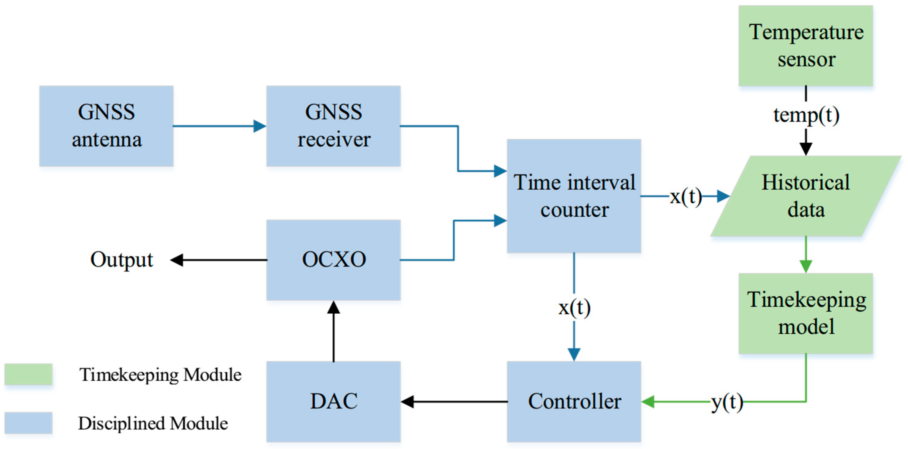
2. OCXO Disciplined and Timekeeping System

As shown in Figure 1, the OCXO disciplined and timekeeping system consists of two parts: the GNSS-disciplined module for the timing phase and the timekeeping module during the timing service interruption phase. The blue arrows indicate the data transmission in the timing phase, which is utilized for parameter estimation and modeling; the green arrows indicate the transmission of data used for estimation in the timing service interruption phase; and the black arrows indicate the control of the OCXO and are shared by both. During the timing phase, the GNSS receiver acquires and decodes the time and frequency signals from the satellite system. The time offset of the OCXO, synchronized with the receiver’s decoded time, is measured by a time interval counter, stored as historical data, and used to discipline the frequency of the OCXO [23]. During the timing service interruption phase, a timekeeping model is established based on the temperature and clock offset data collected during the timing phase. The frequency offset of the OCXO is estimated and compensated for by the model and the real-time temperature.

3. Methodology

3.1. Timekeeping Model for OCXO

As mentioned before, the OCXO is aging and susceptible to temperature, so the timekeeping model during the timing service interruption phase can be expressed as

$$y(t)=y_t(t)+y_{temp}(t)$$

(1)

where $y(t)$ is the total frequency offset at time t, $y_t(t)$ is the frequency offset due to aging at time t, and $y_{temp}(t)$ is the frequency offset due to the temperature at time t.

Currently, aging models include neural networks, the gray model, power finger functions, and polynomial coefficients [25]. Because models such as neural networks and the gray model are computationally large, the IEC recommends the use of logarithmic and polynomial models to evaluate the frequency drift of the crystal clock [17,18]. The OCXO has obvious frequency drift, but the short-term frequency stability is better, and the timing service interruption time is not too long. Therefore, it is appropriate to choose the quadratic polynomial to fit the time offset data for the OCXO under constant temperature conditions [19,22,26], expressed as

$$x_t(t)=a_0+a_{1}t+a_2{t}^2$$

(2)

where $x_t(t)$ is the time offset caused by aging at time t, which gradually increases with time; $a_0$ is the initial time offset; $a_1$ is the relative frequency offset; and $a_2$ is the frequency aging rate.

The relationships between frequency and temperature of quartz crystals of different cut types are different from each other. The frequency–temperature correspondence curve of the AT-cut crystal is roughly three or five times, and the frequency–temperature curve of the crystals of BT, CT, DT, and other cut types is roughly quadratic. The crystals of OCXO clocks are generally SC-cut, with good amplitude–frequency characteristics and small frequency–temperature coefficients [27]. Although the temperature–frequency curve of SC-cut crystals is also nonlinear, the OCXO clock places the crystal and the circuit in a thermostatic bath, and the temperature is controlled at the inflection point where the temperature coefficient is minimized, so that its internal temperature can be controlled to fluctuate within a small range even if the external temperature is changing significantly [20]. In addition, this paper studies OCXO in the natural environment, where the range of the temperature change is small. Therefore, the study assumes that the frequency–temperature curve is linear [12,21,22,28]. The effect of temperature on the frequency can be expressed as

$$y_{temp}(t)=b_0+b_{1}temp(t)$$

(3)

where $b_0$ is the frequency offset caused by the initial temperature, $b_1$ denotes the temperature coefficient, and $temp(t)$ is the temperature at time t.

Assuming that the initial moment $t_1=0$ and the time offset at moment $t_1$ is $x_1$, the relationship between the time offset $x(t)$ and the frequency offset $y(t)$ at moment t is

$$x(t)=x_1+{\displaystyle {\int }_0^{t}y(t)dt}.$$

(4)

Therefore, the frequency offset model for OCXO can be expressed as

$$y(t)=u_t\ast t+u_{temp}\ast temp(t)+u_0$$

(5)

where $u_{temp}$ and $u_t$ represent the temperature and aging coefficients, respectively, and $u_0$ denotes the initial frequency offset. The key to estimating and compensating for the frequency offset of the OCXO during the timing service interruption phase is to accurately estimate the temperature and aging coefficients. When utilizing data from the timing phase for coefficient estimation, the key is to separate the clock offset caused by temperature and aging from the total clock offset obtained in practice [12].

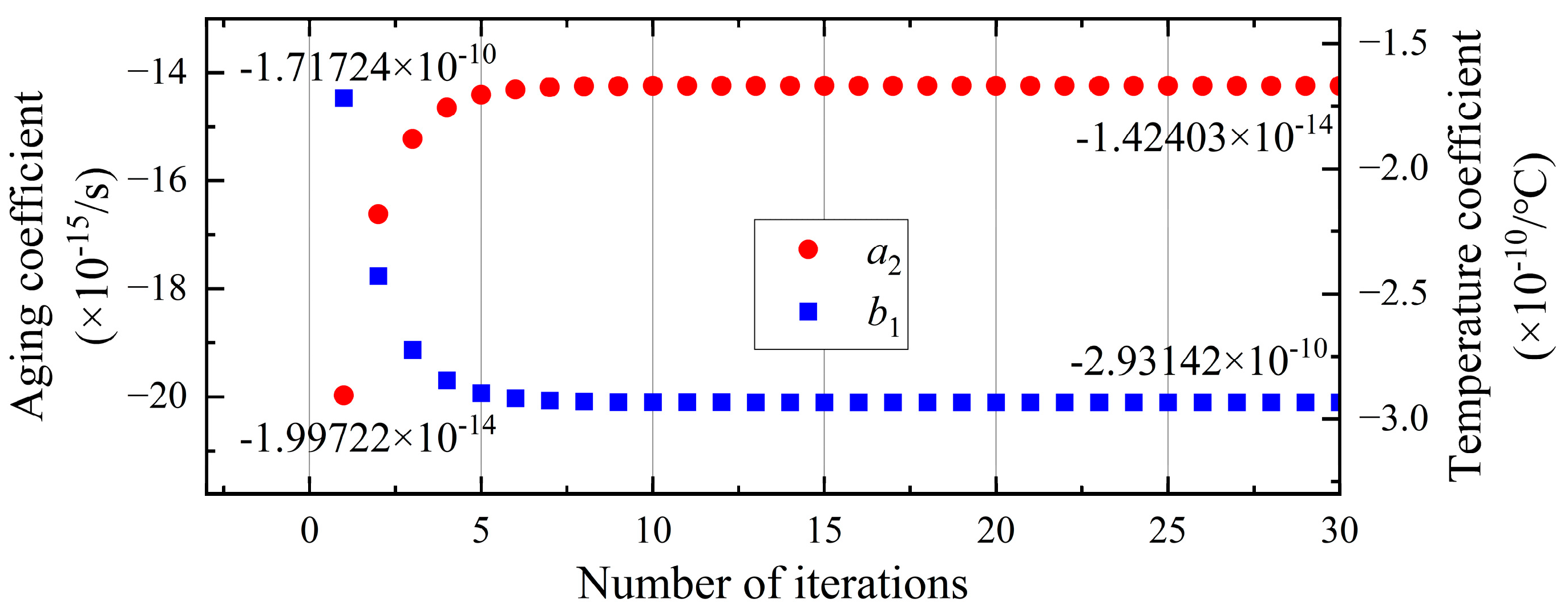
3.2. External Iterative Algorithm

To separate the effects of temperature and aging on the OCXO clock, the clock offset model of the OCXO during the timing phase is expressed as

$$\left\{\begin{array}{l}{x}_t(t)=x(t)-x_{temp}(t)\\ y_{temp}(t)=y(t)-y_t(t)\end{array}\right..$$

(6)

However, actual data that can be directly measured are discrete time offsets. n sets of discrete time offset data of $[t(k),temp(k),x(k),y(k))], k=1,2,\dots ,n(n\ge 3)$ are obtained in the disciplined phase, where k is the k-th sampling point and n is the total number of samples. The vector form of the model is

$$\left\{\begin{array}{l}{\mathit{x}}_{\mathit{t}}=\mathit{x}-{\mathit{x}}_{\mathit{temp}}+{\mathit{\epsilon }}_{\mathit{x}}\\ {\mathit{y}}_{\mathit{temp}}=\mathit{y}-{\mathit{y}}_{\mathit{t}}+{\mathit{\epsilon }}_{\mathit{y}}\end{array}\right.$$

(7)

where $\mathit{x}={[x(1),x(2),\dots ,x(n)]}^T$ is the total time offset vector, and $\mathit{y}={[y(1),y(2),\dots ,y(n-1)]}^T$ is the total frequency offset vector; ${\mathit{x}}_{\mathit{temp}}={[x_{temp}(1),x_{temp}(2),\dots ,x_{temp}(n)]}^T$ and ${\mathit{y}}_{\mathit{t}}={[y_t(1),y_t(2),\dots ,y_t(n-1)]}^T$ are time-offset vectors caused by temperature and frequency offset vectors caused by aging; and ${\mathit{\epsilon }}_{\mathit{x}}$ and ${\mathit{\epsilon }}_{\mathit{y}}$ are the error terms.

An iterative method is employed to separate the effects of temperature and aging, which can be constructed as

$$\left\{\begin{array}{l}{\mathit{x}}_{\mathit{t}}(i)=\mathit{x}-{\mathit{x}}_{\mathit{temp}}(i-1)+{\mathit{\epsilon }}_{\mathit{x}}\\ {\mathit{y}}_{\mathit{temp}}(i)=\mathit{y}-{\mathit{y}}_{\mathit{t}}(i)+{\mathit{\epsilon }}_{\mathit{y}}\end{array}\right.$$

(8)

where ${\mathit{x}}_{\mathit{temp}}(i)$ and ${\mathit{y}}_{\mathit{t}}(i)$ represent the i-th external iteration result of the time offset caused by temperature and the frequency offset caused by aging, respectively. By substituting Equations (2)–(4), the recursive formula from the i-1-th coefficients to the i-th coefficients is:

$$\left\{\begin{array}{l}\mathit{W}\ast \mathit{a}(i)=\mathit{x}-\mathit{C}\ast {\mathit{N}}^{+}\ast \mathit{b}(i-1)+{\mathit{\epsilon }}_{\mathit{x}}\\ \mathit{N}\ast \mathit{b}(i)=\mathit{y}-\mathit{D}\ast \mathit{W}\ast \mathit{a}(i)+{\mathit{\epsilon }}_{\mathit{y}}\end{array}\right.$$

(9)

where $\mathit{W}=\left(\begin{array}{ccc}1& t_1& t_1^2\\ 1& t_2& t_2^2\\ ⋮& ⋮& ⋮\\ 1& t_n& t_n^2\end{array}\right)$, $\mathit{N}=\left(\begin{array}{cc}1& tem{p}_1\\ 1& tem{p}_2\\ ⋮& ⋮\\ 1& tem{p}_{n-1}\end{array}\right)$, ${\mathit{N}}^{+}=\left(\begin{array}{cc}1& tem{p}_1\\ 1& tem{p}_2\\ ⋮& ⋮\\ 1& tem{p}_n\end{array}\right)$, and $\mathit{C}=\left(\begin{array}{cccc}1& 0& \dots & 0\\ 1& 1& \dots & 0\\ ⋮& ⋮& & ⋮\\ 1& 1& \dots & 1\end{array}\right)$ is the n × n order cumulative matrix, and $\mathit{D}=\left(\begin{array}{ccccc}-1& 1& 0& \dots & 0\\ 0& -1& 1& \dots & 0\\ ⋮& ⋮& ⋮& \ddots & ⋮\\ 0& 0& 0& -1& 1\end{array}\right)$ is the n − 1 × n order difference matrix. $\mathit{a}(i)={[a_0(i),a_1(i),a_2(i)]}^T$ and $\mathit{b}(i)={[b_0(i),b_1(i)]}^T$ are the aging and temperature coefficients of the i-th iteration. Its least squares solution is equivalent to the following equation [29]:

$$\left\{\begin{array}{l}{\mathit{W}}^{\mathit{T}}\mathit{W}\ast \mathit{a}(i)={\mathit{W}}^{\mathit{T}}(\mathit{x}-\mathit{C}\ast {\mathit{N}}^{+}\ast \mathit{b}(i-1))\\ {\mathit{N}}^{\mathit{T}}\mathit{N}\ast \mathit{b}(i)={\mathit{N}}^{\mathit{T}}(\mathit{y}-\mathit{D}\ast \mathit{W}\ast \mathit{a}(i))\end{array}\right.$$

(10)

It can be observed that by solving for the temperature and aging coefficients, the respective effects of temperature and aging on the clock offset can be separated. Least squares solutions for the aging coefficients $a_2(i)$ and temperature coefficients $b_1(i)$ have been studied by neural networks, direct matrix inversion, etc. In this study, we solve the coefficients $\mathit{a}(i)$ and $\mathit{b}(i)$ of the i-th external iteration using the internal Gauss–Seidel iterative algorithm. When the iterative number i or the iterative increment ($a_2(i)-a_2(i-1)$ and $b_1(i)-b_1(i-1)$) reaches the threshold, the external iteration is stopped.

3.3. Internal Gauss–Seidel Iterative Algorithm

The Gauss–Seidel iterative algorithm has the advantages of fewer computer storage units, simpler programming, and the original coefficient matrices remaining unchanged during the computation process. It is widely used in large-scale engineering design to find numerical solutions to problems [30]. For the system of the nonsingular equation

$$\mathit{A}\mathit{x}=\mathit{b}$$

(11)

where the diagonal elements of the coefficient matrix A are all nonzero, the Gauss–Seidel iterative algorithm is given by [29]

$$x_i^{(k+1)}={\displaystyle \frac{1}{a_{ii}}}(b_i-{\displaystyle \sum _{j=1}^{i-1}{a}_{ii}{x}_j^{(k+1)}}-{\displaystyle \sum _{j=i+1}^n{a}_{ii}{x}_j^{(k)}}),i=1,2,\dots ,n k=0,1,\dots$$

(12)

where k is the iteration step, n is the dimension of the system, and i is the variable index being updated. Let $\mathit{A}={\mathit{W}}^{\mathit{T}}\mathit{W}$, $\mathit{B}={\mathit{N}}^{\mathit{T}}\mathit{N}$, $\mathit{m}={\mathit{W}}^{\mathit{T}}(\mathit{x}-\mathit{C}\ast {\mathit{N}}^{+}\ast \mathit{b}(i-1))$, and $\mathit{n}={\mathit{N}}^{\mathit{T}}(\mathit{y}-\mathit{D}\ast \mathit{W}\ast \mathit{a}(i))$; substituting into Equation (8), we get

$$\left\{\begin{array}{l}\mathit{A}\ast \mathit{a}(i)=\mathit{m}\\ \mathit{B}\ast \mathit{b}(i)=\mathit{n}\end{array}\right.$$

(13)

This constructs the internal Gauss–Seidel iterative algorithm:

$$\left\{\begin{array}{l}{a}_0^{(j+1)}(i)={\displaystyle \frac{1}{A_{11}}}[m_{11}-A_{12}{a}_1^{(j)}(i)-A_{13}{a}_2^{(j)}(i)]\\ a_1^{(j+1)}(i)={\displaystyle \frac{1}{A_{22}}}[m_{21}-A_{21}{a}_0^{(j+1)}(i)-A_{23}{a}_2^{(j)}(i)]\\ a_2^{(j+1)}(i)={\displaystyle \frac{1}{A_{33}}}[m_{31}-A_{31}{a}_0^{(j+1)}(i)-A_{32}{a}_1^{(j+1)}(i)]\\ b_0^{(j+1)}(i)={\displaystyle \frac{1}{B_{11}}}[n_{11}-B_{12}{b}_1^{(j)}(i)]\\ b_1^{(j+1)}(i)={\displaystyle \frac{1}{B_{22}}}[n_{21}-B_{21}{b}_0^{(j+1)}(i)]\end{array}\right.$$

(14)

where j = 1, 2, 3, … is the number of internal iterations, and $a_0^{(j)}(i)$, $a_1^{(j)}(i)$, $a_2^{(j)}(i)$ and $b_0^{(j)}(i)$, $b_1^{(j)}(i)$ denote the aging and temperature coefficients of the j-th internal Gauss–Seidel iterative algorithm, respectively. When the internal iterative number j or the iterative increment ($a_2^{(j+1)}(i)-a_2^{(j)}(i)$ and $b_1^{(j+1)}(i)-b_1^{(j)}(i)$) reaches the threshold, the internal iteration is stopped, and the aging coefficients $\mathit{a}(i)$ and temperature coefficients $\mathit{b}(i)$ are obtained, which are used to estimate $\mathit{a}(i+1)$ and $\mathit{b}(i+1)$, respectively.

When the iterative number i or the iterative increment reaches the threshold, the external iteration is stopped, and the aging coefficients $a_0,a_1,a_2$ and temperature coefficients $b_0,b_1$ are obtained. Let $u_t=2a_2$ and $u_{temp}=b_1$ be substituted into the frequency offset model, which is used for frequency offset estimation and compensation during the timing service interruption phase, thus enhancing the resilient timekeeping capability of the OCXO.

4. Experimental Validation and Result Analysis

The timekeeping capability of the OCXO during the timing service interruption phase is analyzed to verify the validity of this timekeeping method in Section 4.1, and the effect of the disciplined time is studied in Section 4.2. A GNSS-disciplined rubidium clock and a GNSS-disciplined OCXO were used for the experiment. The GNSS-disciplined rubidium clock was used as the reference, and the GNSS-disciplined OCXO was used for the GNSS-disciplined and timekeeping experiment. The OCXO was OX36D, and the disciplined signal was the actual GNSS signal received by the timing module. The OCXO was placed indoors with changing temperature measured by a thermometer, instead of in a temperature-controlled chamber without changing temperature. The time offset between the OCXO and the rubidium clock was measured using a time interval counter. First, the OCXO was disciplined by the actual GNSS signal. Subsequently, the GNSS signal was interrupted and the time offset of the free state of the OCXO clock was collected. Finally, the frequency offset of the free state was estimated and compensated for by modeling the time-offset data during the timing phase. Two sets of experiments were conducted to verify the timekeeping capability of the method.

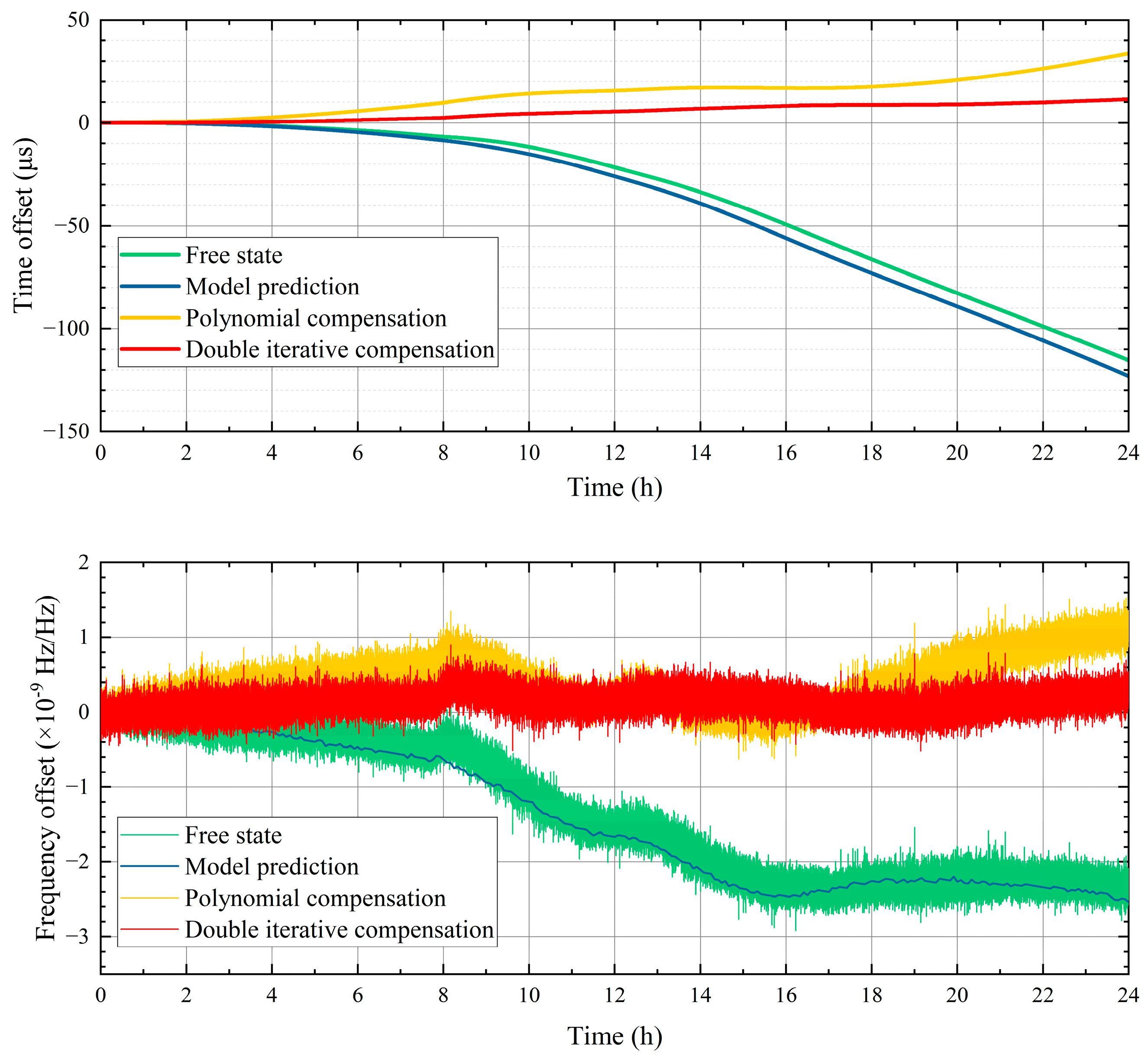
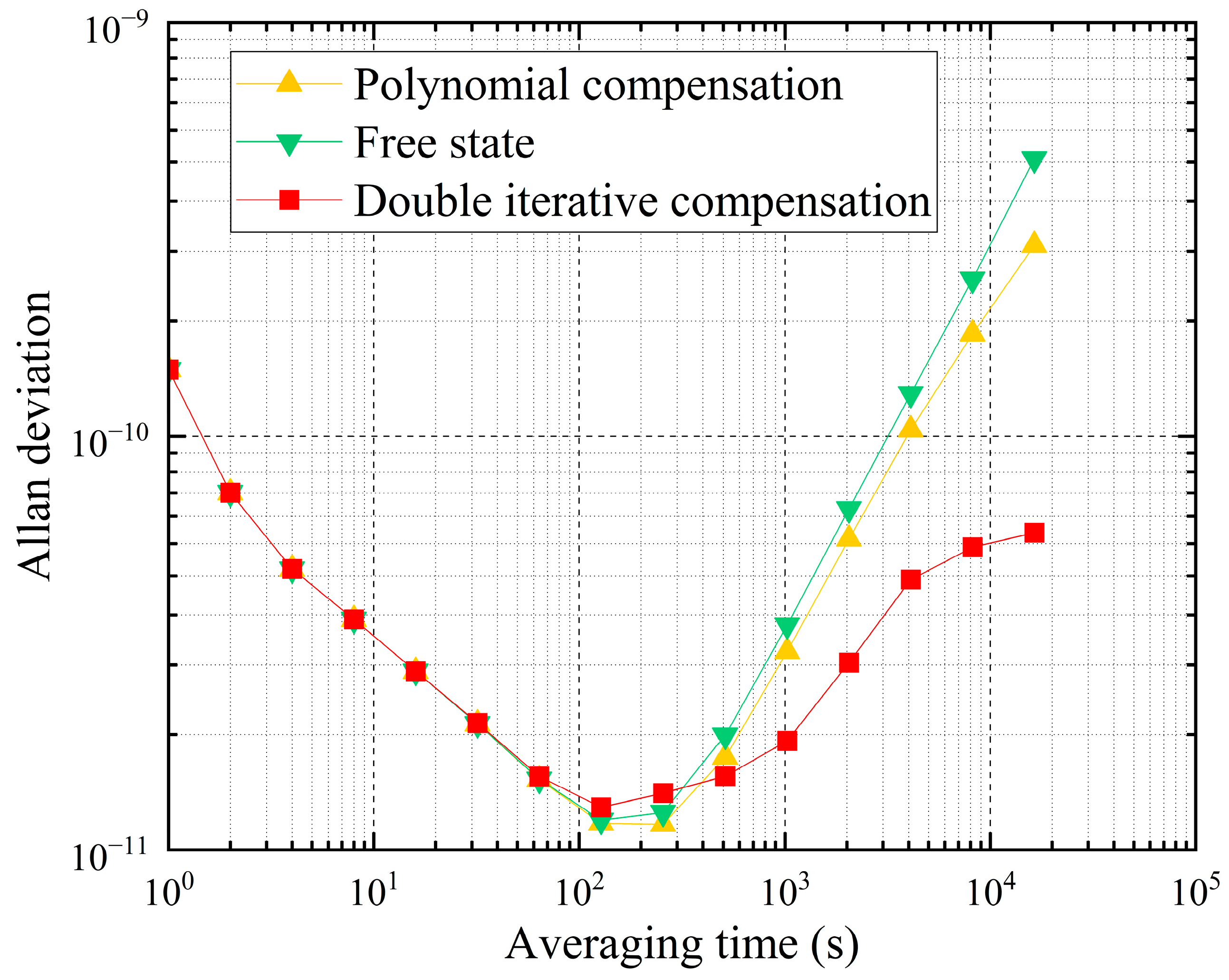
4.1. Experiment to Study the Timekeeping Capability of the Method

To verify the stability of this timekeeping method, we studied whether the temperature and aging coefficients stabilized at the end of the iteration. Without complex calculation capability, the low-cost OCXO clock is not suitable for timekeeping methods such as neural network and machine learning, which have large calculations and complex learning processes. And this timekeeping method is designed for low-cost OCXO and improvement in the second-order polynomial, so we compared it with the second-order polynomial to verify the validity of this timekeeping method.

The model was established using the disciplined data of 24 h during the timing service phase, which separates the clock offset caused by temperature and aging and estimates the coefficients. The results of the coefficients are shown in Figure 2. The initial values of the aging and temperature coefficients were set as 0. The external iterative number and internal iterative number were 30. As shown in Figure 2, the aging coefficient increases and the temperature coefficient decreases as the number of iterations increases. The coefficients are stable at approximately the 10th iteration and finally stabilize at the aging coefficient $a_2=-1.42403\times {10}^{-14}/\mathrm{s}$ and the temperature coefficient $b_1=-2.93142\times {10}^{-14}/℃$.

Using the temperature and aging coefficients, the frequency offset of OCXO during the timing service interruption phase was estimated and compensated. Its timekeeping capability was compared with the free state and second-order polynomial model. The clock offset of OCXO during the timing service interruption phase is shown in Figure 3. As can be seen in Figure 3, the time offset of the OCXO for 24 h is −115.36 μs in the free state, and it is 33.73 μs after being compensated by the second-order polynomial model. The time offset is 11.48 μs after dual iterative algorithm compensation, which improves the time accuracy by 90.05% and 65.97% relative to the free state and the second-order polynomial model, respectively. The frequency offset at 24 h of the OCXO in the free state is −2.2374 × 10⁻⁹, the frequency offset after second-order polynomial model compensation is 1.2137 × 10⁻⁹, and the frequency offset after compensation by the proposed dual iterative algorithm is 3.9896 × 10⁻¹⁰, which improves the frequency accuracy by 82.17% and 67.13% for the free state and second-order polynomial model, respectively.

Table 1. Frequency drift rate during timing service interruption phase.

	Free State	Second-Order Polynomial	Proposed Method
Drift rate of frequency (/s)	−3.48 × 10−14	5.15 × 10−15	8.33 × 10−16
Improvement percentage		85.20%	97.61%

shows the frequency drift rate during the timing service interruption phase. It can be observed that the OCXO after compensation of the proposed algorithm reduces the frequency drift rate by 97.16% and 83.83% for the free-state and second-order polynomial models, respectively.

Figure 4 shows the stability of the OCXO during the timing service interruption phase. There is a typical “flickering plateau” [31] near the smoothing time of 100 s. At τ < 64 s, the Allan deviations of the three statuses were not significantly different. The Allan deviation of the dual iterative algorithm was slightly larger than that of the pre-compensated and second-order polynomial model at 64 s ≤ τ < 512 s. In the comparative analysis for τ ≥ 512 s, the stability of the OCXO after the compensation of the method shows an advantage, which is significantly improved compared with the free-state and second-order polynomial model, which verifies the capability of the model to compensate the frequency drift. The optimization effect on the long stability is further quantified in

Table 2. Optimization ratio of stability during the timing service interruption phase.

Tau	512	1024	2048	4096	8192	16,384
Free state (×10−11)	1.89	3.50	6.68	12.7	24.0	46.9
Compensated (×10−11)	1.51	1.84	2.84	4.50	5.39	5.85
Improvement (%)	20.45	47.52	57.52	64.47	77.49	87.53

, from which it can be seen that after the compensation of the model, the stability improvement ratio η gradually increases with smoothing time relative to the OCXO in the free state. The value of η is 20.45% when τ = 512 s, η is 47.52% when τ = 1024 s, and η is 87.53% when τ = 16,384 s; that is, the model’s improvement in the long-term stability is more obvious, especially when τ > 2048 s, when the optimization is more than 50%.

4.2. Effect of Disciplined Time on Timekeeping Capability

To study the impact of disciplined time on the OCXO timekeeping capability, we established 4 models using 24 h, 48 h, 72 h, and 96 h disciplined datasets. These models were then applied to compensate for free-state OCXO during the timing service interruption phase. Figure 5 shows the time offset improvement results. Figure 6 presents the frequency offset metrics (including mean, standard deviation, median, and maximum values) of the proposed model.

As shown in Figure 5, when the disciplined time was increased from 24 h to 48 h and 72 h, the time offset decreased from 11.48 μs to 0.38 μs and 0.48 μs after timing service interruption for 24 h. Conversely, when the disciplined time was increased to 96 h, the time offset did not continue to decrease but instead increased to 2.10 μs. In other words, further extension of the disciplined time does not lead to substantial improvement in the time offset.

As shown in Figure 6, four frequency offset metrics of the proposed method are all better than OCXO in the free state. The mean, median, and max frequency offset for 48 h, 72 h, and 96 h disciplined times show marked improvement compared with the 24 h results. However, the standard deviation is bigger with the increased disciplined time.

Table 3. Drift rates for different disciplined times.

	Free State	24 h	48 h	72 h	96 h
Drift rate (×10−15/s)	−34.8	0.833	−2.04	−2.30	−2.88
Improvement (%)		97.61	94.15	93.40	91.73

shows the frequency drift rate for different disciplined times, which indicates that the compensation timekeeping method proposed in this passage improves the frequency drift. Through comparative analysis of four different disciplined times (24 h, 48 h, 72 h, and 96 h), it was found that the improvement in frequency drift rate after compensation exceeded 90% (specifically, ranging from 91.73% to 97.61%). As the disciplined time increased, the absolute value of the drift rate showed a monotonic upward trend. Specifically, when the disciplined time extended from 24 h to 96 h, the drift rate increased from 8.33 × 10⁻¹⁶/s to 2.88 × 10⁻¹⁵/s, representing an increase of approximately 2.5 times. This result aligns with the observation that the absolute value of time offset first decreases and then increases after being disciplined for 96 h. This is possibly due to other factors of the OCXO changing over time, causing minor fluctuations in aging and temperature parameters, which suggests that an appropriate disciplined time should be selected during modeling.

According to the results of Section 4.1, the effect of this model in the range of short-term stability (τ < 125 s) is not obvious, so Figure 7 shows the system’s performance when τ ≥ 125 s. The x-axis is the smoothing time τ, and the y-axis is the Allan deviation of different disciplined times (24 h, 48 h, 72 h, 96 h). When τ < 4096 s, there is no significant difference in the frequency stability among the four disciplined times. As τ increases to 16,384 s, the Allan deviations of 96 h are significantly higher than the Allan deviations of 24 h. The Allan deviations of 96 h and 24 h are 6.7495 × 10⁻¹¹ and 5.8460 × 10⁻¹¹, respectively, and their difference is 9.035 × 10⁻¹², which is up to 15.46%. In other words, increased disciplined time may result in higher long-term stability.

Figure 8 shows the time offset at different moments during the timing service interruption phase. The x-axis is the timing service interruption time, and the y-axis is the time offset at the moment. Different colors represent the time offsets with different models. As shown in Figure 8, after using the timekeeping method, the time offsets for 1, 2, 5, 12 s and 24 h are less than 0.07 μs, 0.09 μs, 0.81 μs, 5.34 μs, and 11.48 μs, respectively. When the interruption time is less than 2 h, OCXO disciplined for 24 h shows better timekeeping performance. As the timing service interruption time increases, OCXO with a longer disciplined time performs better. For example, after 1 h, the time offset of OCXO disciplined for 24 h was 0.032 μs, which improved by 48.4% compared with OCXO disciplined for 48 h (0.062 μs). After 5 h, the time offset of OCXO disciplined for 24 h was 0.807 μs, while that of the OCXO disciplined for 48 h was 0.179 μs. After 24 h, the offset further expanded to 11.48 μs (disciplined for 24 h) versus 0.38 μs (disciplined for 48 h).

Table 4. Improvement of clock offset for different disciplined times.

Experiment	Free State (μs)	Compensation (24 h)		Compensation (48 h)		Compensation (72 h)		Compensation (96 h)
		Bias (μs)	Radio	Bias (μs)	Radio	Bias (μs)	Radio	Bias (μs)	Radio
1	98.97	35.44	64.19%	4.57	95.38%	1.63	98.36%	0.55	99.45%
2	87.49	7.89	90.98%	0.58	99.34%	0.40	99.54%	0.05	99.94%
3	74.88	8.98	88.01%	4.44	94.07%	0.96	98.72%	3.37	95.50%
4	91.02	19.41	78.68%	9.49	89.58%	6.22	93.17%	3.05	96.65%
5	115.36	11.48	90.04%	0.38	99.67%	0.48	99.58%	2.10	98.18%

shows the time offset and the improvement in five experiments with different disciplined times after timing service interruption for 24 h. As shown in Table 4, the time offset of free-state OCXO exceeded 70 μs over 24 h. After modeling by disciplined data of 24, 48, 72, and 96 h, the time offsets were reduced to less than 40 μs, 10 μs, 7 μs, and 4 μs, respectively.

5. Conclusions

This paper presents a timekeeping method with a dual iterative algorithm for GNSS-disciplined OCXO during the timing service interruption phase. This method estimates temperature and aging coefficients of GNSS-disciplined OCXO during the timing phase and estimates and compensates for real-time frequency offset during the timing service interruption phase. Experimental results demonstrated some improvements in time offset, frequency offset, frequency drift rate, and long-term stability. Modeling with 24 h, 48 h, 72 h, and 96 h disciplined data, time offsets were less than 40 μs, 10 μs, 7 μs, and 4 μs after 24 h, representing an improvement of more than 60%, 85%, 90%, and 95%, respectively, while the time offset of OCXO in the free state was more than 70 μs.

References

1. Meng, Y.S.; Lei, W.Y.; Bian, L.; Yan, T.; Wang, Y. Clock tuning technique for a disciplined high medium–long-stability GNSS oscillator with precise clock drifts for LEO users. GPS Solut. 2020, 24, 110. [Google Scholar] [CrossRef]
2. Huang, Y.; Zhang, X.W.; Cong, L.; Dong, X.H. Time synchronization error analysis and evaluation of TH-2 satellite. Acta Geod. Cartogr. Sin. 2022, 51, 2455–2461. [Google Scholar]
3. Liu, Y.M. Research and Design of Key Technologies for Physical Layer to 5G V2X Standardization. Ph.D. Thesis, Beijing University of Posts and Telecommunications, Beijing, China, 2019. [Google Scholar]
4. Sun, H.J.; Wu, Y.Y.; Zhang, J.X. Attitude synchronization control for multiple spacecraft: A preassigned finite-time scheme. Adv. Space Res. 2024, 73, 6094–6110. [Google Scholar] [CrossRef]
5. Ba, X.; Liu, T.; Jiang, W.; Wang, J. Design of Universal Code Generator for Multi-Constellation Multi-Frequency GNSS Receiver. Electronics 2024, 13, 1244. [Google Scholar] [CrossRef]
6. Abedi, A.A.; Mosavi, M.R. Low Computational-Complexity vector tracking for Low-Cost GNSS receivers. Measurement 2022, 195, 111171. [Google Scholar] [CrossRef]
7. Eghtesadi, M.; Mosavi, M.R. A Pseudo-Differential LNA with Noise Improvement Techniques for Concurrent Multi-Band GNSS Applications. Electronics 2024, 13, 2805. [Google Scholar] [CrossRef]
8. Wang, J.; Yu, X.; Guo, S. Inversion and characteristics of unmodeled errors in GNSS relative positioning. Measurement 2022, 195, 111151. [Google Scholar] [CrossRef]
9. China Crystal Vibrators in Consumer Electronics Industry Market Space Measurement 2023. Available online: https://wenku.baidu.com/view/52098505b007e87101f69e3143323968011cf439.html?_wkts_=1752744636839 (accessed on 16 September 2023).
10. Shi, C.; Zheng, F.; Lou, Y.; Wang, Y.; Zhang, A.; Zhang, S.; Zhang, D.; Song, W.; Wang, M.; Lin, Y.; et al. Theoretical approach and application of BeiDou high-precision time-frequency service. J. Wuhan Univ. Inf. Sci. Ed. 2023, 48, 1010–1018. [Google Scholar]
11. Wang, Q.; Peng, L.F. Constant temperature crystal taming method based on GPS/BDS dual mode receiver. GNSS World China 2021, 46, 1–4. [Google Scholar]
12. Lu, G. Research on GNSS Disciplined Crystal Oscillator and Holdover Technologies. Ph.D. Thesis, University of Chinese Academy of Sciences, Beijing, China, 2021. [Google Scholar]
13. Yang, Y.X.; Ren, X.; Jia, X.L.; Sun, B.J. Development trends of the national secure PNT system based on BDS. Sci. China Earth Sci. 2023, 53, 917–927. [Google Scholar] [CrossRef]
14. Zhao, S.H.; Zhao, Y. Crystal Oscillator; Science Publishing House: Beijing, China, 2008. [Google Scholar]
15. Wang, X.; Yang, Y.; Wang, B.; Lin, Y. Resilient timekeeping algorithm with multi-observation fusion Kalman filter. Satell. Navig. 2023, 4, 25. [Google Scholar] [CrossRef]
16. Wang, X.; Yang, Y.; Lin, Y.; Wang, B.; Han, C. Resilient evaluation algorithm of caesium fountain clock based on robust adaptive observation model. Phys. Scr. 2023, 98, 115411. [Google Scholar] [CrossRef]
17. DIN EN IEC 62884-3; Measurement Techniques of Piezoelectric, Dielectric and Electrostatic Oscillators—Part 3: Frequency Aging Test Methods (IEC 62884-3:2018). German Version EN IEC 62884-3:2018. 2018. Available online: https://standards.cencenelec.eu/dyn/www/f?p=CENELEC:110:::::FSP_PROJECT,FSP_ORG_ID:64599,1258061&cs=10CCB2865C70EC9844C7794C8CE72DCBB (accessed on 15 July 2025).
18. Xue, C. Analysis on Characteristics and Standard Demand of Crystal Oscillator Analysis on Characteristics and Standard Demand of Crystal Oscillator. China Stand. 2020, 201, 153–157. [Google Scholar]
19. Fan, D.S.; Liu, Y.; Li, X.H. Crystal oscillator disciplined method based on Kalman filter. Time Freq. 2019, 42, 224–229. [Google Scholar]
20. Jia, Y.J. Study on the Taming and Holding Technology of the Oven Controlled Crystal Oscillator. Ph.D. Thesis, Xidian University, Xi’an, China, 2021. [Google Scholar]
21. Li, H. Research on High Stability Crystal Taming and Holding System Based on GPS 1PPS. Ph.D. Thesis, Xi’an University of Science and Technology, Xi’an, China, 2023. [Google Scholar]
22. Guo, W.F.; Gong, Q.R.; Zhu, M.M.; Shi, C. Method and performance of time timekeeping for RT-PPT receivers utilizing on-line estimation of clock parameters. GPS Solut. 2024, 28, 201. [Google Scholar] [CrossRef]
23. Li, H.Y.; Zhang, Y.J. A Greedy Gauss-Seidel Method for Solving the Large Linear Least Squares Problem. Tongji Univ. Nat. Sci. 2021, 49, 1514–1521. [Google Scholar]
24. Kunzi, F.; Montenbruck, O. Precise disciplined of a chip-scale atomic clock using PPP with broadcast ephemerides. GPS Solut. 2023, 27, 165. [Google Scholar] [CrossRef]
25. Gong, Y.Y. Analysis of Atomic Clock Performance and Clock Difference Prediction Algorithm. Master’s Thesis, Xi’an University of Science and Technology, Xi’an, China, 2021. [Google Scholar]
26. Huang, G.W. Research on Algorithms of Precisie Clock Offset and Quality Evaluation of GNSS Satellite Clocks A. Ph.D. Thesis, Chang’an University, Xi’an, China, 2012. [Google Scholar]
27. Jackson, G.S. Method and Apparatus to Improve Performance of GPSDO’s and Other Oscillators. U.S. Patent US8362845 B2, 29 January 2013. [Google Scholar]
28. Zuo, Z.Y. Research on a Clock Disciplining and Holding System Based on Beidou Time Service. Ph.D. Thesis, Xidian University, Xi’an, China, 2022. [Google Scholar]
29. Guan, Z.; Lu, J.F. Fundamentals of Numerical Analysis, 3rd ed.; Higher Education Press: Beijing, China, 2010; pp. 79–82. [Google Scholar]
30. Li, A.Q. Iterative solution of systems of linear equations. Sci. Technol. Eng. 2007, 14, 3357–3364. [Google Scholar]
31. Wang, Y.Q. Atomic Clocks and Time-Frequency Systems: An Anthology; National Defense Industry Press: Beijing, China, 2012. [Google Scholar]
Figure 1. OCXO disciplined and timekeeping system [24].
Electronics 14 02870 g001
Figure 2. Coefficients during dual iterative algorithm.
Electronics 14 02870 g002
Figure 3. Clock offset during timing service interruption phase.
Electronics 14 02870 g003
Figure 4. Stability during the timing service interruption phase.
Electronics 14 02870 g004
Figure 5. Time offset for different disciplined times.
Electronics 14 02870 g005
Figure 6. Frequency offset statistics for different disciplined times.
Electronics 14 02870 g006
Figure 7. Stabilization with different disciplined time.
Electronics 14 02870 g007
Figure 8. Time offset at different moments.
Electronics 14 02870 g008