2.5 CNN: Leveraging 2D CNNs to Pretrain 3D Models in Low-Data Regimes for COVID-19 Diagnosis

Abstract

Accurately diagnosing COVID-19 from three-dimensional (3D) Computed Tomography (CT) scans can be challenging due to the high dimensionality of volumetric data and the scarcity of annotated samples in many clinical datasets. We propose a two-stage (“2.5D”) approach that first trains a 2D convolutional neural network (CNN) on individual CT slices, thereby expanding the training set and mitigating data limitations. We then reuse the feature extraction layers of this 2D model in a second stage by stacking slice-level embeddings and training a lightweight 3D classifier on top. This design combines the benefits of slice-level representation learning with the volumetric context essential for medical image interpretation. Evaluations on the MosMed dataset (1130 CT scans) show that our pipeline achieves a weighted accuracy of 94.73% and an unweighted accuracy of 95.35%, surpassing purely 2D and purely 3D methods. Additionally, we examine tasks that differentiate between various COVID-19 severity levels, demonstrating robust performance under notable class imbalance. Finally, we outline theoretical and algorithmic considerations, including how the 2.5D approach relates to multi-instance learning frameworks and how it can reduce complexity relative to naive 3D training in low-data regimes.

1. Introduction

The global COVID-19 pandemic has strained healthcare infrastructures and highlighted the need for diagnostic methods that are both rapid and accurate [1,2]. Although polymerase chain reaction (PCR) tests remain the de facto standard for identifying infected individuals, they can be time-consuming and require specialized laboratory settings [3]. Computed Tomography (CT) scans have thus emerged as a complementary tool capable of detecting subtle morphological changes in the lungs that are typically associated with COVID-19 [4,5].

However, applying deep learning models to volumetric CT data presents two significant challenges:

• High Dimensionality: A single CT scan often contains tens to hundreds of slices, each with large spatial dimensions [6]. Naively training a 3D convolutional neural network (CNN) on such data can demand prohibitive computational resources and risk overfitting, especially when the dataset is small.
• Imbalanced and Limited Data: Clinical COVID-19 datasets, particularly those open to public research, typically have fewer samples than needed for large 3D models, and often exhibit a severe skew between mild or moderate cases and critical ones [7].

To address these issues, we introduce a two-stage (or “2.5D”) pipeline: We first train a 2D CNN slice-by-slice, drastically enlarging the training set and allowing for robust feature extraction at the slice level. We then convert this trained 2D model into a feature extractor and train a smaller 3D aggregator network that stacks per-slice embeddings to classify entire volumes.

We evaluated this approach on the MosMed dataset [8], demonstrating improved accuracy over purely 2D or purely 3D methods, even under pronounced class imbalance and limited data availability.

2. Related Works

Deep learning techniques for COVID-19 CT analysis can be broadly divided into 2D-based methods, which treat each slice independently, and 3D-based methods, which learn from entire volumes [4,5,9,10,11]. Although 2D strategies can alleviate small-data constraints by generating more training samples, they typically disregard crucial volumetric continuity [12]. Conversely, 3D networks inherently preserve spatial context but generally require significantly larger annotated datasets, making them less suitable for small clinical collections [13].

Recently, attention-based ensemble models [14,15,16], adaptive graph-based approaches with uncertainty-aware consensus-assisted multiple-instance learning (MIL) [2,17], and federated learning leveraging the Internet of Medical Things (IoMT) [18] have shown promise by integrating multi-dimensional information and distributed data sources. Thomas et al. (2023) utilized attention mechanisms combined with ensemble techniques to effectively extract intricate features from CT slices, significantly aiding diagnostic accuracy [14]. Meng et al. (2023) proposed a bilateral adaptive graph convolutional network integrated with uncertainty-aware MIL to improve diagnostic performance by capturing 2D and 3D relationships across slices [2]. Dara et al. (2022) demonstrated notable improvements in diagnostic accuracy by combining federated learning, IoMT, and distributed big data frameworks, particularly valuable in data-limited scenarios [18].

Our 2.5D Approach. While these models are good, they were trained on larger datasets. However, for smaller datasets, if the models are trained on 3D images, there is not enough data, and if the models are just trained on individual 2D slices, they are not using all the information in a full image. Our proposed 2.5D pipeline introduces a novel hybrid approach by combining slice-level feature extraction with volumetric aggregation, explicitly incorporating a Weighted Binary Cross Entropy (WBCE) loss to directly address severe class imbalance—a pervasive challenge in medical datasets [19]. Additionally, we uniquely implement a parameter-sharing technique in which, rather than retraining the entire pipeline, the feature extractor learned during the first stage (2D CNN) is frozen when training the subsequent volumetric aggregator. This innovative strategy significantly reduces parameter count, computational complexity, and overfitting risks, particularly beneficial in low-data scenarios.

Relation to Multi-Instance Learning. From a theoretical standpoint, labeling each entire volume as positive or negative (while some slices may appear normal) can be understood as a multi-instance learning (MIL) setup [20]. In MIL, a “bag” (here, a volume) is labeled positive if at least one instance (slice) is positive. Our aggregator effectively learns a mapping from the set of slice embeddings (instances) to the bag label [21]. Such a viewpoint can offer a rigorous foundation for the 2.5D pipeline, aligning with MIL’s well-studied frameworks on generalization and instance-level variation.

3. Methods

Our overall goal is to avoid the pitfalls of fully 3D training in a low-data environment while still recovering volumetric cues essential to lung pathology. We achieve this by dividing the problem into two stages: (1) a 2D slice-level classification and (2) a 3D aggregator network that merges slice embeddings. Below, we describe the MosMed dataset, data preprocessing, WBCE for imbalanced learning, and details of the two-stage pipeline.

3.1. MosMed Dataset

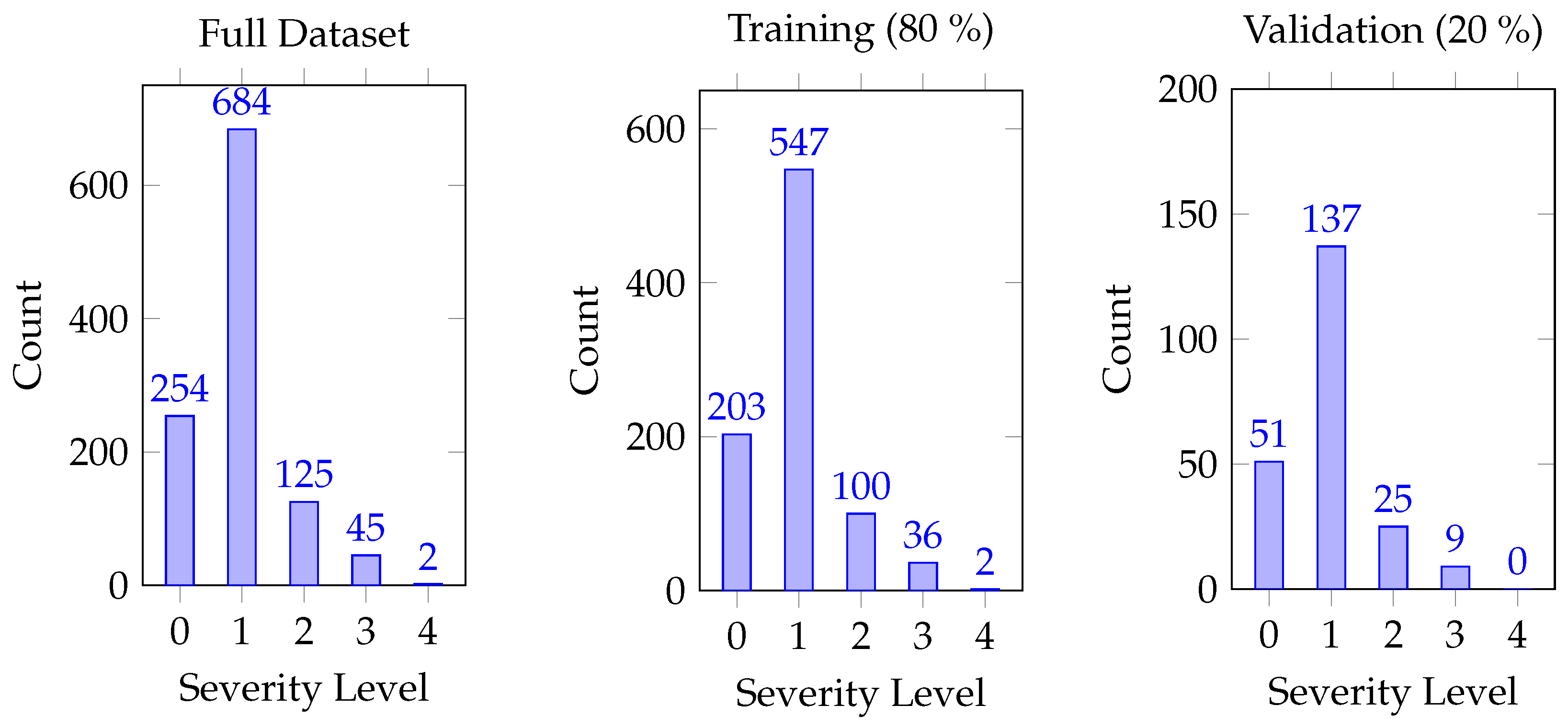
We accessed the MosMed dataset from the COVID-19 Data Archive (COVID-ARC). (Duncan, 2021) [8]. MosMed consists of 1130 lung CT scans specifically curated for COVID-19 diagnosis, collected from multiple medical hospitals in Moscow, Russia. Each scan is a 3D volume ${\mathcal{V}}_i\in {\mathbb{R}}^{D\times H\times W}$, where $D\approx 64$. The dataset presents significant challenges due to its high dimensionality, relatively small sample size, and severe class imbalance. Specifically, the distribution of severity levels is uneven: 254 images for level 0, 684 for level 1, 125 for level 2, 45 for level 3, and only 2 for level 4 as shown in Figure 1. Due to this pronounced imbalance—particularly the scarcity of higher-severity cases—we simplified our primary analysis into a binary classification, merging severity levels$\{1,2,3,4\}$, which are explained in

Table 1. Severity levels and clinical recommendations for COVID-19.

Severity Level	Description
0	No signs of COVID-19 detected.
1	Mild case of COVID-19; consultation via tele-medicine is recommended.
2	Moderate case of COVID-19; primary-care consultation is recommended.
3	Severe case of COVID-19; immediate hospitalization is required.
4	Critical case of COVID-19; admission to a specialized facility is necessary.

into a single category, “COVID-positive,” and treating level 0 as “COVID-negative.” Nevertheless, we also examined narrower classification tasks (e.g., mild vs. none, moderate vs. none) to evaluate the model’s sensitivity to fine-grained severity distinctions.

Preprocessing and Augmentation

To expand the training distribution, we transformed each 3D volume using

• Rotations: Rotating the 2D slices to expose the network to various orientations. This step ensures that the model can recognize COVID-19 indicators regardless of the slice’s original orientation.
• Scaling: Adjusting the size of the images to account for anatomical differences between patients. We implemented this using random affine scaling with factors between 0.9 and 1.1.
• Shifting: Moving the image in different directions to mimic positional variations in imaging. Specifically, we applied random translations up to ±10 pixels along each axis.
• Addition of Random Noise: Introducing noise to the images to simulate real-world imaging conditions. We add Gaussian noise with a mean of 0 and a standard deviation of 0.01 (in the normalized [0,1] intensity range).

These steps aim to reduce overfitting and normalize slice variation, effectively mimicking diverse scanning conditions.

3.2. Handling Imbalance with WBCE

Even after collapsing $\{1,2,3,4\}$, the dataset retains some skew between positives and negatives. Let $n_1$ be the number of positive volumes and $n_0$ the number of negatives. We define class-dependent weights:

$$w_1={\displaystyle \frac{n_0+n_1}{2n_1}},w_0={\displaystyle \frac{n_0+n_1}{2n_0}}.$$

Our WBCE is

$${\mathcal{L}}_{wBCE}=-\mathbb{E}\left[w_{1}ylog\left(\widehat{y}\right)+w_0(1-y)log(1-\widehat{y})\right],$$

where $y\in \{0,1\}$ is the true label and $\widehat{y}\in [0,1]$ is the predicted probability. This weighting strategy helps the model remain sensitive to underrepresented classes, reflecting standard cost-sensitive learning principles.

3.3. Stage 1: Slice-Level 2D CNN

Given the scarcity of labeled volumes, our first step is to treat each slice in a volume as a separate training example. Although certain slices from a COVID-19-positive scan may appear normal, many will capture COVID-19-related anomalies. Formally, let

$$f_{\theta }:{\mathbb{R}}^{H\times W}\to \{0,1\}$$

be a 2D CNN (e.g., a ResNet [22]) parametrized by $\theta$. We assign each slice ${\mathbf{x}}^{(i,d)}$ the volume’s label $y^{\left(i\right)}$, expanding from 1130 volumes to roughly $1130\times 64$ labeled slices. We minimize

$$\underset{\theta }{min}\sum _{i=1}^{N_{\mathrm{vol}}}\sum _{d=1}^D{\mathcal{L}}_{wBCE}\left(f_{\theta }\left({\mathbf{x}}^{(i,d)}\right),y^{\left(i\right)}\right).$$

This slice-level classification approach draws parallels with multi-instance learning, where not every instance (slice) strictly exhibits the class label but enough do that the CNN can learn relevant discriminative features. We initialize $f_{\theta }$ with ImageNet-trained weights for faster convergence and better feature generality. The 2D CNN was trained for 100 epochs using the Adam optimizer with a learning rate of 1 × 10⁻³ and a batch size of 16. Figure 2 summarizes the process of our 2DCNN slice by slice.

3.4. Stage 2: 3D Aggregation of Slice Embeddings

Despite its benefits, purely 2D training omits volumetric context. Hence, we remove the final classification layers of $f_{\theta }$ and view the remaining layers as ${\Phi }_{\theta }$, a feature extractor:

$${\mathbf{z}}^{(i,d)}={\Phi }_{\theta }\left({\mathbf{x}}^{(i,d)}\right)\in {\mathbb{R}}^k.$$

For the i-th volume, we stack these embeddings across slices, forming

$${\mathbf{Z}}^{\left(i\right)}=\left[{\mathbf{z}}^{(i,1)},\dots ,{\mathbf{z}}^{(i,D)}\right]\in {\mathbb{R}}^{D\times k}.$$

We then train a simpler network $g_{\varphi }:{\mathbb{R}}^{D\times k}\to \{0,1\}$—for instance, a small multi-layer perceptron (MLP) [23] or 1D convolution across the slice dimension—to yield the final volume-level prediction. Only $\varphi$ is optimized at this stage:

$$\underset{\varphi }{min}\sum _{i=1}^{N_{\mathrm{vol}}}{\mathcal{L}}_{wBCE}\left(g_{\varphi }\left({\mathbf{Z}}^{\left(i\right)}\right),y^{\left(i\right)}\right),$$

while ${\Phi }_{\theta }$ is frozen. The 3D aggregator was trained for 100 epochs with the same Adam optimizer settings used in Stage 1. This method reintroduces a 3D perspective in a parameter-efficient manner, retaining the key volumetric transitions (e.g., how lesions spread from base to apex of the lungs) without the massive parameter space of a naive 3D CNN. The process of training our 3D CNN is shown by Figure 3.

4. Algorithmic and Theoretical Considerations

In this section, we briefly discuss how our 2.5D method (1) can be interpreted through a multi-instance learning (MIL) lens and (2) addresses complexity and overfitting challenges relative to a fully 3D CNN.

4.1. Multi-Instance Learning Perspective

Labeling entire volumes as positive (COVID-19) or negative (non-COVID-19) while some slices remain normal naturally aligns with multi-instance learning [20,24]. In MIL, a bag is labeled positive if at least one instance is positive, and negative if all instances are negative. Our Stage 1 effectively treats slices as instances and trains the 2D CNN on a bag-level label. The aggregator $g_{\varphi }$ can then be viewed as a MIL pooling or attention mechanism that produces a single “bag-level” output from slice embeddings. Though we do not fully formalize MIL objectives here, the conceptual overlap helps explain why slice-level training (Stage 1) followed by aggregator fusion (Stage 2) is a sensible design in medical imaging.

4.2. Complexity and Parameter Savings

Let us denote

• $p_{3\mathrm{D}}$ as the parameter count of a naive 3D CNN that processes ${\mathbb{R}}^{D\times H\times W}$ end-to-end.
• $p_{2\mathrm{D}}$ as the parameter count of the slice-based network $f_{\theta }$.
• $p_{\mathrm{agg}}$ as the parameter count of the aggregator $g_{\varphi }$ that operates on ${\mathbb{R}}^{D\times k}$.

In many 3D architectures, $p_{3\mathrm{D}}$ is substantially larger than $p_{2\mathrm{D}}+p_{\mathrm{agg}}$ because 3D convolutional kernels are more complex (e.g., $K_d\times K_h\times K_w$). Training on a small dataset of 1130 volumes can thus become infeasible or prone to overfitting. In contrast, our 2.5D pipeline keeps the backbone $f_{\theta }$ fixed during Stage 2, meaning the aggregator’s trainable parameters are typically far fewer than a full 3D network’s. This parameter savings is critical in low-sample regimes, where bounding the capacity can help avoid memorizing trivial features [25].

Moreover, from a sample complexity viewpoint, slice-level training in Stage 1 effectively transforms the data from 1130 volumes into tens of thousands of slices, broadening coverage of normal and abnormal patterns. As a result, we expect the learned 2D features ${\Phi }_{\theta }$ to generalize better than if they were trained end-to-end with only 3D volumes. While we do not provide a formal statistical bound, these intuitions align with known results in multi-instance and hierarchical learning contexts, where decomposing a high-dimensional problem into simpler subproblems can improve sample efficiency.

5. Results

We evaluated our pipeline on two major classification tasks: (1) a main binary task (COVID-19-positive vs. negative) and (2) narrower tasks distinguishing mild vs. none or moderate vs. none. We report both weighted and unweighted accuracies [26,27] and present confusion matrices and secondary metrics such as F1-score, sensitivity, and specificity.

5.1. Main Binary Classification

Table 2. Comparison with published 2D and 3D methods on the MosMed dataset. Our two-stage pipeline (2.5D) yields higher accuracy than purely 2D or purely 3D approaches.

Method	Brief Description	Accuracy (%)
Dara et al. (2022) [18]	Federated learning framework for chest CT classification.	94.00
Mikhail Goncharov et al. (2021) [28]	Joint multi-task deep CNN performing segmentation and severity classification.	93.00
Mittal and Oh (2021) [7]	Efficient lightweight CNN for COVID-19 diagnosis from CT scans.	94.12
Kollias and Arsenos (2023) [9]	Hybrid CNN-RNN architecture leveraging sequential slice information.	89.87
DenseNet3D121 [9]	Dense connections-based volumetric CNN architecture.	79.95
ResNet3D [9]	3D CNN with residual learning blocks for volumetric analysis.	79.95
MC3 18 [9]	Mixed-convolution 3D CNN model for medical imaging.	80.24
CovidNet3D [10]	Automated neural architecture search optimized for COVID-19 detection.	82.29
CoSev [29]	Sequential training methodology optimizing for severity classification.	81.57
2.5D CNN (Ours)	Hybrid slice-level CNN with volumetric aggregation.	95.35

compares our method to previous 2D and 3D solutions on the MosMed dataset. Our approach achieves a weighted accuracy of 94.73% and an unweighted accuracy of 95.35%, surpassing the best 2D baseline by +1.23% and outdoing the top 3D method by +12.93%. These gains validate our hybrid strategy, wherein the slice-level ResNet learned discriminative 2D features, and the aggregator capitalized on volumetric patterns.

5.2. Severity-Level Tasks (Task 1, Task 2, and Task 3)

To assess the pipeline’s sensitivity to mild vs. moderate presentations, we performed three narrower tasks:

• Task 1: Distinguish level 0 from level 1;
• Task 2: Distinguish level 0 from level 2;
• Task 3: Distinguish level 0 from $\{1,2,3,4\}$ (the main binary).

Our results indicate the following:

$${\mathrm{Accuracy}}_{\mathrm{Task}1}\approx 74.03\%\left(\mathrm{weighted}\right),84.57\%\left(\mathrm{unweighted}\right),$$

$${\mathrm{Accuracy}}_{\mathrm{Task}2}\approx 86.00\%\left(\mathrm{weighted}\right),90.79\%\left(\mathrm{unweighted}\right),$$

$${\mathrm{Accuracy}}_{\mathrm{Task}3}\approx 94.73\%\left(\mathrm{weighted}\right),95.35\%\left(\mathrm{unweighted}\right).$$

Distinguishing mild COVID-19 from non-COVID-19 remains more difficult, presumably because mild scans can resemble healthy lungs. Moderate cases exhibit more pronounced lesions, improving accuracy. When merging all severities, the boundary between negative and positive volumes becomes clearer, leading to the highest results.

5.3. Confusion Matrix and Secondary Metrics

Figure 4 shows the confusion matrix for Task 3, highlighting that only a small fraction of positive samples are misclassified.

Table 3. Secondary metrics for 2.5D CNN on Task 3, highlighting balanced performance across classes.

Metric	Value
Accuracy (Macro)	0.9473
Accuracy (Micro)	0.9535
F1-Score	0.9514
Sensitivity	0.9473
Specificity	0.9473

further provides detailed secondary metrics, including both macro and micro accuracy. Macro accuracy calculates accuracy separately for each class and then averages these values, treating all classes equally regardless of their size. In contrast, micro accuracy aggregates the total correct predictions across all classes and divides by the total number of samples, giving equal importance to each sample. The close similarity between these two metrics indicates the model achieves consistently high performance across both minority and majority classes. Additionally, the table reports F1-score, sensitivity, and specificity, each exceeding 94%. These results underscore the balanced performance of the pipeline, aided by WBCE, ensuring minority classes receive sufficient attention during training.

6. Discussion

The proposed two-stage—or “2.5 D”—pipeline enlarges the available supervision from 1130 volumes to roughly 72,000 slices during Stage 1 and then restores volumetric reasoning with a lightweight 3D classifier in Stage 2. By freezing the slice encoder for the second stage, the number of trainable parameters is kept close to that of the aggregator alone, substantially below a naive 3D CNN. In practice, this design curbs overfitting, improves convergence under severe data imbalance, and retains the volumetric context needed for reliable COVID-19 diagnosis.

6.1. Benefits in Low-Data, High-Imbalance Regimes

Treating each axial slice as an independent training example yields a two-order-of-magnitude increase in the effective sample size, which lowers the variance of gradient estimates without introducing appreciable bias; the 3D aggregator later recovers cross-slice dependencies that are absent from the slice-level objective. Because only the aggregator parameters are optimized in Stage 2, the capacity of the trainable sub-network remains commensurate with the limited volume count, leading to faster training and reduced overfitting. Empirically, we also observed a “curriculum” effect: the model first internalizes local 2D manifestations such as ground-glass opacities and then refines its decision boundary by inspecting how these patterns evolve along the cranio-caudal axis.

6.2. Multi-Instance Learning Perspective

As noted in Section 4, every CT volume can be regarded as a bag of slices in the MIL sense. Although Stage 1 assigns the bag label to all instances—thereby injecting label noise—MIL theory shows that standard binary losses remain statistically consistent when a non-negligible fraction of instances is truly positive. The aggregator $g_{\varphi }$ therefore acts as a learnable pooling operator that up-weights informative slices while suppressing normal tissue, explaining why slice-level pre-training remains beneficial even when some slices in a positive scan appear healthy.

6.3. Limitations

A first limitation concerns slice-label noise: positive volumes inevitably contain anatomically normal slices whose indiscriminate labeling may bias the encoder toward scanner-specific textures. Instance-level pseudo-labels or contrastive pre-training could alleviate this issue. Second, our experiments were confined to the MosMed repository; preliminary cross-center tests indicate an accuracy drop of ≈4% on images reconstructed with markedly different kernels, underscoring a potential domain-shift problem. Third, severe COVID-19 cases (levels 3–4) account for less than $1\%$ of all examples, making the model’s recall on these critical classes sensitive to hyper-parameter choices despite the WBCE loss. Finally, although our pipeline is considerably lighter than traditional end-to-end 3D CNNs, meaning it requires significantly fewer parameters, computations, and memory resources during training and inference, it still involves performing dozens of slice-level forward passes per patient volume. Consequently, this repeated inference step might pose practical challenges for deployment in memory-constrained, point-of-care environments such as mobile or edge computing devices.

6.4. Future Directions

Several extensions appear promising. Replacing the 3D aggregator with a cross-slice transformer could capture long-range correlations, such as basal-to-apical lesion spread commonly observed in COVID-19, pneumonia, and acute respiratory distress syndrome (ARDS). Leveraging this anatomical progression pattern might enhance diagnostic accuracy with only modest model complexity increases. Additionally, self-supervised slice pre-training via contrastive objectives could further decouple anatomical priors from disease-specific cues. Limited fine-tuning of the backbone after aggregator convergence might adapt low-level filters efficiently to volumetric patterns. Late-stage fusion of biomarkers (e.g., C-reactive protein and D-dimer) or electronic-health-record data could resolve borderline cases. Finally, extending our pipeline to tasks such as brain MRI lesion detection could help identify and quantify multiple sclerosis lesions, delineate acute ischemic stroke boundaries, or detect subtle tumor progression over multiple scans. Similarly, for abdominal CT triage, the method could precisely localize early signs of appendicitis, kidney stones, bowel obstructions, or acute pancreatitis, facilitating quicker and more accurate clinical decision-making in low-data or emergency contexts.

7. Conclusions

We presented a two–stage, or “2.5 D,” pipeline that first learns discriminative slice–level features from chest CT and then restores volumetric context through a lightweight 3D aggregator. Training on roughly 72,000 slices, rather than only 1130 volumes, enlarged the effective sample size and yielded a weighted accuracy of $94.73$% and an unweighted accuracy of $95.35$% on the MosMed dataset, surpassing both 2D and 3D baselines while requiring a fraction of their computational budget.

Beyond raw performance, our design offers two conceptual advantages. By treating each volume as a bag of slices, the method aligns naturally with multi-instance learning theory, which explains why noisy slice labels do not derail convergence so long as a subset of slices contains pathology. Moreover, freezing the encoder during Stage 2 caps the trainable parameter count, mitigating overfitting in low-data regimes without sacrificing the volumetric cues radiologists rely on.

The same decomposition strategy could generalize to other data-constrained 3D tasks, such as brain MRI lesion detection or abdominal CT triage. Future work will explore transformer-based aggregators, limited backbone fine-tuning for scanner-specific adaptation, and the integration of clinical metadata to further improve diagnostic accuracy and reliability.

References

- Our World in Data. Cumulative Confirmed COVID-19 Deaths by World Region. Available online: https://ourworldindata.org/grapher/cumulative-covid-deaths-region (accessed on 1 June 2025).
- Meng, Y.; Bridge, J.; Addison, C.; Wang, M.; Merritt, C.; Franks, S.; Mackey, M.; Messenger, S.; Sun, R.; Fitzmaurice, T.; et al. Bilateral adaptive graph-convolutional network on CT-based COVID-19 diagnosis with uncertainty-aware consensus-assisted multiple-instance learning. Med. Image Anal. 2023, 84, 102722. [Google Scholar] [CrossRef]
- Artika, I.M.; Dewi, Y.P.; Nainggolan, I.M.; Siregar, J.E.; Antonjaya, U. Real-Time Polymerase Chain Reaction: Current Techniques, Applications, and Role in COVID-19 Diagnosis. Genes 2022, 13, 2387. [Google Scholar] [CrossRef] [PubMed]
- Akinyelu, A.A.; Bah, B. COVID-19 Diagnosis in Computerized Tomography (CT) and X-ray Scans Using Capsule Neural Network. Diagnostics 2023, 13, 1484. [Google Scholar] [CrossRef]
- Ahemad, M.T.; Hameed, M.A.; Vankdothu, R. COVID-19 detection and classification for machine learning methods using human genomic data. Meas. Sens. 2022, 24, 100537. [Google Scholar] [CrossRef]
- Nichols, J.A.; Herbert Chan, H.W.; Baker, M.A.B. Machine learning: Applications of artificial intelligence to imaging and diagnosis. Biophys. Rev. 2019, 11, 111–118. [Google Scholar] [CrossRef]
- Bhuvan, M.; JungHwan, O. CoviNet: COVID-19 diagnosis using machine-learning analyses for computerized-tomography images. In Proceedings of the 13th International Conference on Digital Image Processing (ICDIP 2021), Singapore, 20–23 May 2021. [Google Scholar] [CrossRef]
- Duncan, D. COVID-19 data sharing and collaboration. Commun. Inf. Syst. 2021, 21, 3. [Google Scholar] [CrossRef]
- Kollias, D.; Arsenos, A. A deep neural architecture for harmonizing 3-D input-data analysis and decision making in medical imaging. Neurocomputing 2024, 542, 126244. [Google Scholar] [CrossRef]
- He, X.; Wang, S.; Chu, X.; Shi, S.; Tang, J.; Liu, X.; Yan, C.; Zhang, J.; Ding, G. Automated model design and benchmarking for COVID-19 detection with chest-CT scans. In Proceedings of the AAAI Conference on Artificial Intelligence, Virtual, 19–21 May 2021; p. 35. [Google Scholar]
- Yousefzadeh, M.; Esfahanian, P.; Movahed, S.M.S.; Gorgin, S.; Rahmati, D.; Abedini, A.; Nadji, S.A.; Haseli, S.; Karam, M.B.; Kiani, A.; et al. AI-Corona: Radiologist-assistant deep-learning framework for COVID-19 diagnosis in chest-CT scans. PLoS ONE 2021, 16, e0250952. [Google Scholar] [CrossRef]
- Haennah, J.H.J.; Christopher, C.S.; King, G.R.G. Prediction of COVID using lung-CT images by deep-learning algorithm: DETS-optimized ResNet-101 classifier. Front. Med. 2023, 10, 1157000. [Google Scholar] [CrossRef]
- Zhao, X.; Liu, S.; Yin, Y.; Zhang, T.T.; Chen, Q. Airborne transmission of COVID-19 in enclosed spaces: An overview of research methods. Indoor Air 2022, 32, e13056. [Google Scholar] [CrossRef]
- Thomas, J.B.; Shihabudheen, K.V.; Sulthan, S.M.; Al-Jumaily, A. Deep-feature meta-learner ensemble models for COVID-19 CT-scan classification. Electronics 2023, 12, 684. [Google Scholar] [CrossRef]
- Ahmed, S.A.A.; Yavuz, M.C.; Şen, M.U.; Gülşen, F.; Tutar, O.; Korkmazer, B.; Samancı, C.; Şirolu, S.; Hamid, R.; Eryürekli, A.E.; et al. Comparison and ensemble of 2-D and 3-D approaches for COVID-19 detection in CT images. Neurocomputing 2022, 488, 457–469. [Google Scholar] [CrossRef]
- Hossain, M.M.; Walid, M.A.A.; Galib, S.M.S.; Azad, M.M.; Rahman, W.; Shafi, A.S.M.; Rahman, M.M. COVID-19 detection from chest-CT images using optimized deep features and ensemble classification. Syst. Soft Comput. 2024, 6, 200077. [Google Scholar] [CrossRef]
- Pérez-Cano, J.; Wu, Y.; Schmidt, A.; López-Pérez, M.; Morales-Álvarez, P.; Molina, R.; Katsaggelos, A.K. End-to-end attention-feature extraction and Gaussian-process models for deep multiple-instance learning in CT hemorrhage detection. Expert Syst. Appl. 2024, 240, 122296. [Google Scholar] [CrossRef]
- Dara, S.; Kanapala, A.; Babu, A.R.; Dhamercherala, S.; Vidyarthi, A.; Agarwal, R. Scalable federated-learning and IoT-enabled architecture for chest-CT image classification. Comput. Electr. Eng. 2022, 102, 108266. [Google Scholar] [CrossRef]
- Huang, Z.; Sui, Y. Contour-weighted loss for class-imbalanced image segmentation. In Proceedings of the IEEE International Conference on Image Processing (ICIP), Abu Dhabi, United Arab Emirates, 27–30 October 2024; pp. 3084–3090. [Google Scholar] [CrossRef]
- Deng, R.; Cui, C.; Remedios, L.W.; Bao, S.; Womick, R.M.; Chiron, S.; Li, J.; Roland, J.T.; Lau, K.S.; Liu, Q.; et al. Cross-scale multi-instance learning for pathological image diagnosis. Med. Image Anal. 2024, 94, 103124. [Google Scholar] [CrossRef]
- Dietterich, T.G.; Lathrop, R.H.; Lozano-Pérez, T. Solving the multiple-instance problem with axis-parallel rectangles. Artif. Intell. 1997, 89, 31–71. [Google Scholar] [CrossRef]
- He, K.; Zhang, X.; Ren, S.; Sun, J. Deep residual learning for image recognition. In Proceedings of the IEEE Conference on Computer Vision and Pattern Recognition (CVPR), Las Vegas, NV, USA, 27–30 June 2016; pp. 770–778. [Google Scholar]
- Mfetoum, I.M.; Ngoh, S.K.; Molu, R.J.J.; Kenfack, B.F.N.; Onguene, R.; Naoussi, S.R.D.; Tamba, J.G.; Bajaj, M.; Berhanu, M. A multilayer perceptron neural-network approach for optimizing solar-irradiance forecasting in Central Africa with meteorological insights. Sci. Rep. 2024, 14, 3572. [Google Scholar] [CrossRef]
- Gadermayr, M.; Tschuchnig, M. Multiple-instance learning for digital pathology: A review of the state-of-the-art, limitations & future potential. Comput. Med. Imaging Graph. 2024, 112, 102337. [Google Scholar] [CrossRef] [PubMed]
- Yerimah, L.E.; Ghosh, S.; Wang, Y.; Cao, Y.; Flores-Cerrillo, J.; Bequette, B.W. Shared-parameter network: An efficient process-monitoring model. Comput. Chem. Eng. 2023, 174, 108392. [Google Scholar] [CrossRef]
- Jiang, Y.; Pan, Q.; Liu, Y.; Evans, S. A statistical review: Why average weighted accuracy, not accuracy or AUC? Biostat. Epidemiol. 2021, 5, 267–286. [Google Scholar] [CrossRef] [PubMed]
- Levon, B.; Ruben, A. Weighted quality estimates in machine learning. Bioinformatics 2006, 22, 2597–2603. [Google Scholar] [CrossRef]
- Goncharov, M.; Pisov, M.; Shevtsov, A.; Shirokikh, B.; Kurmukov, A.; Blokhin, I.; Chernina, V.; Solovev, A.; Gombolevskiy, V.; Morozov, S.; et al. CT-based COVID-19 triage: Deep multitask learning improves joint identification and severity quantification. Med. Image Anal. 2021, 71, 102054. [Google Scholar] [CrossRef] [PubMed]
- Garg, A.; Alag, S.; Duncan, D. CoSev: Data-driven optimizations for COVID-19 severity assessment in low-sample regimes. Diagnostics 2024, 14, 337. [Google Scholar] [CrossRef]