Mitigating Class Imbalance Challenges in Fish Taxonomy: Quantifying Performance Gains Using Robust Asymmetric Loss Within an Optimized Mobile–Former Framework

Abstract

Accurate fish species identification is crucial for marine biodiversity conservation, environmental monitoring, and sustainable fishery management, particularly as marine ecosystems face increasing pressures from human activities and climate change. Traditional morphological identification methods are inherently labor-intensive and resource-demanding, while contemporary automated approaches, particularly deep learning models, often suffer from significant computational overhead and struggle with the pervasive issue of class imbalance inherent in ecological datasets. Addressing these limitations, this research introduces a novel computationally parsimonious fish classification framework leveraging the hybrid Mobile–Former neural network architecture. This architecture strategically combines the local feature extraction strengths of convolutional layers with the global context modeling capabilities of transformers, optimized for efficiency. To specifically mitigate the detrimental effects of the skewed data distributions frequently observed in real-world fish surveys, the framework incorporates a sophisticated robust asymmetric loss function designed to enhance model focus on under-represented categories and improve resilience against noisy labels. The proposed system was rigorously evaluated using the comprehensive FishNet dataset, comprising 74,935 images distributed across a detailed taxonomic hierarchy including eight classes, seventy-two orders, and three-hundred-forty-eight families, reflecting realistic ecological diversity. Our model demonstrates superior classification accuracy, achieving 93.97 percent at the class level, 88.28 percent at the order level, and 84.02 percent at the family level. Crucially, these high accuracies are attained with remarkable computational efficiency, requiring merely 508 million floating-point operations, significantly outperforming comparable state-of-the-art models in balancing performance and resource utilization. This advancement provides a streamlined, effective, and resource-conscious methodology for automated fish species identification, thereby strengthening ecological monitoring capabilities and contributing significantly to the informed conservation and management of vital marine ecosystems.

1. Introduction

The accurate identification and classification of aquatic species represent a fundamental prerequisite for robust environmental monitoring, effective fishery management, and the broader goals of ecological conservation [1,2,3]. Amidst the escalating pressures from global climate change and diverse anthropogenic activities, the health and stability of marine ecosystems are subjects of increasing international concern. Precise species-level data are indispensable for tracking biodiversity trends, assessing the impacts of environmental perturbations, and formulating scientifically grounded conservation and management strategies [4]. Within the domain of fisheries, accurate taxonomic classification is equally critical, underpinning sustainable practices through informed quota setting, the protection of vulnerable or endangered species, and the overall maintenance of resource viability [5].

Historically, fish classification has predominantly relied upon manual identification by trained experts. While foundational, manual identification inherently faces significant limitations in scalability and efficiency. These methods demand considerable human resources and scarce taxonomic expertise, and they are often too time-consuming for the large image volumes from modern ecological surveys, thereby hindering timely data acquisition and analysis [6]. The logistical constraints of manual identification thus pose a bottleneck to timely data acquisition and analysis.

The advent of computer vision and the subsequent rise of deep learning techniques have offered powerful alternatives, driving a paradigm shift towards automated image recognition methods [7,8,9]. These automated systems promise substantial reductions in human intervention and significant improvements in classification throughput, especially when dealing with large-scale datasets [10]. The early successes demonstrated the potential of applying sophisticated feature analysis, including deep feature recognition, to classify fish effectively even within challenging underwater contexts [11]. Further research has continued to explore and refine intelligent classification techniques based on data-driven learning, capable of discerning complex patterns directly from image data without reliance on hand-crafted features [12,13]. Such methods have demonstrably enhanced classification accuracy and reduced the manual labeling burden, facilitating a greater focus on model refinement and application deployment [14].

Despite these advancements, the automated classification of fish species in situ presents persistent challenges. The sheer diversity of aquatic life results in vast inter-species variations in size, morphology, and coloration, demanding highly discriminative models [15]. Furthermore, the underwater imaging environment itself introduces complexities: variable lighting conditions, water turbidity, and cluttered backgrounds can severely degrade image quality and consistency, negatively impacting model performance and generalization [16]. A critical challenge, particularly in ecological datasets, is class imbalance. This phenomenon, characterized by long-tailed distributions where many species have few samples, often biases model training towards common species [17]. Concurrently, the increasing complexity of state-of-the-art deep learning models often translates to substantial computational costs and significant memory footprints, posing practical barriers for deployment on resource-constrained platforms, such as autonomous underwater vehicles or edge devices. Achieving model lightweighting while preserving high accuracy remains a key research imperative.

In response to these multifaceted challenges, this paper introduces an efficient and lightweight fish classification model engineered to balance high performance with computational feasibility while explicitly addressing the problem of class imbalance. The core contributions of this work are enumerated as follows:

• We propose and implement a lightweight fish classification model based on the Mobile–Former architecture. This design minimizes computational complexity (FLOPs) and model parameters without sacrificing significant classification accuracy, enhancing the suitability for deployment in resource-limited scenarios.
• To counteract the adverse effects of data imbalance intrinsic to ecological datasets, we integrate an advanced robust asymmetric loss function. This component specifically enhances the model’s sensitivity to minority classes, thereby promoting more equitable recognition across the taxonomic spectrum and improving the overall classification robustness.
• We conduct extensive empirical validation on the publicly accessible FishNet dataset. Comparative analyses demonstrate the superiority of our proposed model against the existing methods across standard evaluation metrics. Furthermore, ablation studies are performed to rigorously dissect the contribution of each architectural and methodological component to the final observed performance.

The rest of this paper is organized as follows: Section 2 reviews the related work in the field of aquatic species classification and hybrid CNN and ViT architectures. Section 3 details the FishNet dataset utilized in our study, including its structure and characteristics. Section 4 presents the design and methodology of the proposed lightweight fish classification model, Mobile–Former, and discusses the robust asymmetric loss function employed to tackle the class imbalance issue. Section 5 describes the experimental setup, evaluates the model’s performance, and compares it with the existing approaches. Finally, Section 6 provides concluding remarks and a discussion regarding future research directions.

2. Related Work

2.1. Aquatic Species Classification

With the rapid advancement of computer vision technology, automated fish classification methods have gradually become a popular topic in the research community. These methods significantly improve the efficiency of fish identification, particularly in handling large amounts of image data and real-time monitoring, demonstrating clear advantages. Traditional fish classification methods rely on manual feature extraction and pattern recognition; however, these methods often struggle to cope with the vast diversity of fish species, similar appearances, and the complex underwater environment. To overcome these challenges, researchers have focused on developing more advanced algorithms and models to enhance classification accuracy and stability [18]. Furthermore, addressing the long-tail distribution inherent in species datasets remains an active area of research, with recent advancements focusing on techniques like decoupled training [19], re-weighting strategies such as Balanced Softmax [20], and novel loss functions designed to better handle imbalanced data.

Currently, machine-learning-based and deep-learning-based fish classification methods have been widely applied. For example, Salman et al. [11] achieved remarkable classification performance by employing deep feature recognition to classify fish in underwater images. Gomes et al. [21] explored automated fish classification methods based on convolutional neural networks (CNNs) and confirmed their reliability in complex marine environments. Zhao et al. [14] conducted a systematic review of recent deep learning techniques, highlighting their applications across various fish habitats and their species recognition capabilities, while also pointing out the dependency on large amounts of labeled data. Additionally, researchers have noted the impact of background diversity on fish classification. Catalan et al. [22] investigated the “domain shift” issue, where models trained in one environment perform poorly in a new setting—a phenomenon particularly evident in fish classification due to underwater lighting changes and complex backgrounds that significantly affect model generalization. To address this issue, methods such as data augmentation, transfer learning, and multi-task learning have been proposed to improve model performance across different backgrounds.

2.2. Hybrid CNN and ViT Architectures

Hybrid models that combine convolutional neural networks (CNNs) and Vision Transformers (ViTs) have recently gained significant attention in the field of computer vision [23,24,25]. This hybrid architecture aims to integrate the strengths of both approaches while overcoming their individual limitations, thereby enhancing the performance of image processing tasks. These architectures can be broadly categorized into parallel integration, serial integration, and hierarchical integration.

Parallel integration architectures leverage the strengths of both CNNs and ViTs by processing the same input data in parallel, thereby capturing both local features and global contextual information during processing. For instance, the Conformer architecture proposed by Peng et al. [26] is a typical parallel integration model that aligns and fuses the local features extracted by CNNs with the global information captured by ViTs using an innovative Feature Combination Unit, leading to better image processing performance than using single models like ResNet or DeiT.

On the other hand, serial integration architectures process input data initially through one architecture and then pass the output as an input to the next architecture for continuous feature extraction and processing. For example, CETNet [27] integrates CNNs and ViTs by introducing Convolutional Embedding and Local Enhanced Window Self-Attention mechanisms, achieving excellent performance in the ImageNet-1k image classification task. Similarly, CoAtNet [28] connects ViT modules after multiple MobileNetV2 modules, combining the local feature extraction capability of CNNs with the global context awareness of ViTs, thereby maintaining high generalization even with limited data.

Hierarchical integration architectures fuse the functionalities of CNNs and ViTs at different levels of data processing to maximize the advantages of each level. For example, ViTAE [29] introduces spatial pyramid down-sampling modules and convolutional blocks into the ViT model to achieve hierarchical feature extraction, attaining state-of-the-art performance on the ImageNet dataset. CvT [30] replaces the positional encoding of ViTs and integrates the spatial information of CNNs, achieving significant results in image recognition tasks, while DiNAT [31] introduces an expanded neighborhood attention mechanism to reduce computational complexity and enhance image recognition performance. DiNAT further reduces computational complexity while improving the understanding of the global context.

3. FishNet Dataset

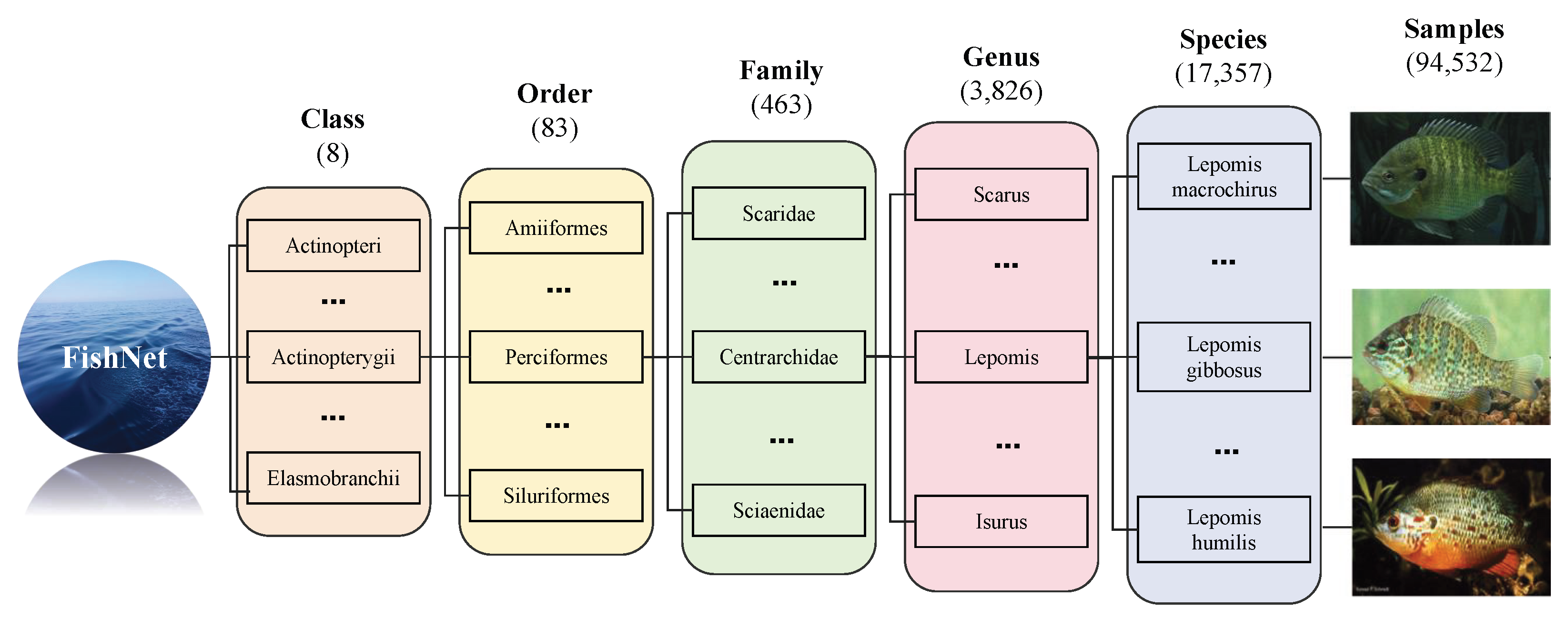
In this study, we utilized a large-scale aquatic species identification dataset named FishNet [32], designed to support researchers and decision-makers in better understanding and preserving biodiversity. The FishNet dataset meticulously collected 94,532 high-quality images from various global aquatic environments, encompassing 17,357 species of aquatic organisms. These organisms are organized according to a scientifically recognized aquatic taxonomy system (class, order, family, genus, and species), with corresponding images supporting each classification. This provides a rich foundation for training and validating deep learning models. Furthermore, to address common issues in datasets, such as limited species counts and the lack of functional trait data, FishNet has been significantly expanded in both quantity and diversity. It not only includes common species but also covers some less common or understudied species, greatly broadening its potential application scope. Figure 1 presents samples of the dataset.

In constructing the FishNet dataset, to ensure broad applicability and research value, we specifically excluded families with fewer than 10 samples at the subfamily level. This measure aims to enhance the accuracy and reliability of the dataset when used for fish classification. By this screening process, we ensured that each family has a sufficient number of samples to support the training of complex machine learning algorithms. Ultimately, the dataset includes 74,935 images across 8 taxonomic classes, 72 orders, and 348 families. At the family level, the dataset exhibits a characteristic long-tail distribution. While the most populous families comprise thousands of images, many others are under-represented. Specifically, among the 348 families, 65 (approx. 18.7%) contain 50 or fewer samples, and a subset of 20 families (approx. 5.7%) are under-represented with 10 or fewer samples, qualifying as extreme long-tail categories. This imbalance underscores the challenge for robust classification across all taxonomic groups and highlights the need for specialized evaluation of model performance on these rare categories.

Table 1. The 15 orders with the most samples and the 15 orders with fewest samples.

Family	Count	Family	Count
Labridae	4782	Trichomycteridae	71
Pomacentridae	3430	Auchenipteridae	68
Cyprinidae	3354	Gadidae	67
Centrarchidae	2908	Mormyridae	66
Gobiidae	2540	Ogcocephalidae	66
Cichlidae	2302	Petromyzontidae	66
Sparidae	1876	Zoarcidae	66
Salmonidae	1833	Gastromyzontidae	65
Serranidae	1828	Amphiliidae	62
Acanthuridae	1446	Opistognathidae	62
Syngnathidae	1356	Polynemidae	62
Sciaenidae	1312	Stomiidae	61
Percidae	1174	Belonidae	58
Scaridae	1090	Goodeidae	58
Monacanthidae	1077	Hemiramphidae	58

presents the 15 orders with the most samples and the 15 orders with the fewest samples, where we can see the dataset’s significant long-tail distribution.

4. Model and Methods

We designed and implemented a lightweight fish classification model based on Mobile–Former, which reduces computational complexity and model parameters while maintaining high classification accuracy, making it suitable for resource-constrained practical applications. Additionally, to address the class imbalance problem, this paper proposes an improved asymmetric loss function that effectively enhances the model’s ability to recognize minority classes, thereby improving the overall classification performance.

4.1. Mobile–Former Overall Architecture

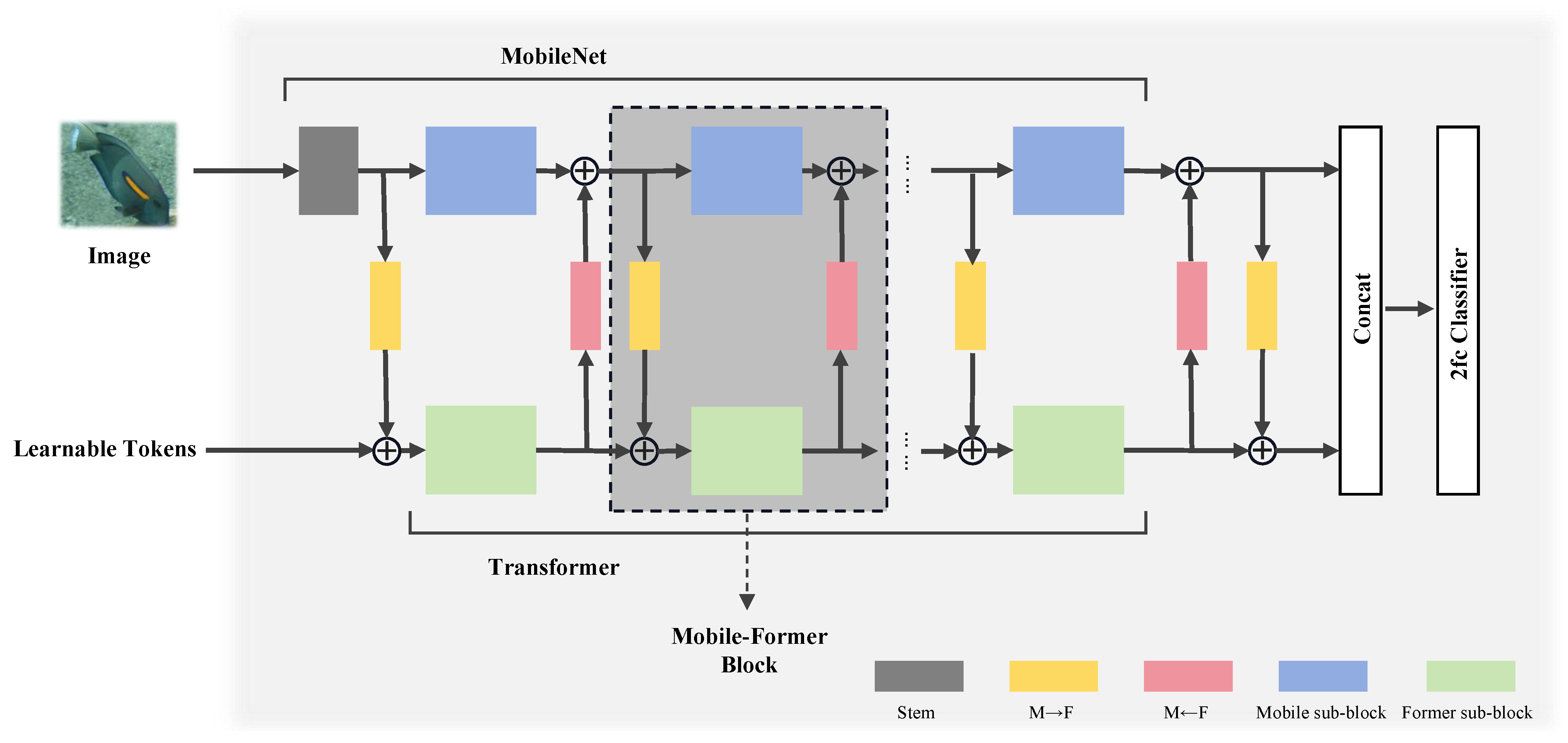
In modern image classification tasks, effectively integrating local and global information is key to improving recognition performance. Mobile–Former [33] is an innovative network architecture that achieves a parallel design between MobileNet and a transformer through bidirectional bridging. This design leverages MobileNet’s efficiency in local processing and the powerful capability of transformers in global interactions. It is acknowledged that the bidirectional cross-attention mechanism, while powerful for feature fusion, can introduce additional parallel computation overhead compared to purely sequential architectures. To mitigate this in resource-constrained deployments, future optimizations could explore operator fusion techniques, such as those inspired by FasterBlock optimizations, to merge consecutive operations and reduce memory access and kernel launch overhead, thereby potentially further improving inference speed on edge devices. This structure not only enhances the model’s ability to handle complex visual tasks but also maintains relatively low computational costs, making it particularly suitable for resource-constrained environments. The overall architecture of Mobile–Former used in our work is shown in Figure 2.

The core idea of Mobile–Former is to achieve feature fusion between MobileNet and a transformer through a bidirectional bridge (bidirectional cross-attention mechanism). In Mobile–Former, the MobileNet component is responsible for processing the input image, utilizing its efficient depthwise convolution and pointwise convolution to extract rich local features. Meanwhile, the transformer component processes a small number of learnable tokens designed to capture global information from the image. Specifically, the input tokens to the transformer component are $Z\in {\mathbb{R}}^{M \times d}$, where M is the number of tokens, and d is the dimension of each token. These tokens are processed through a self-attention mechanism and a Feed-Forward Network (FFN).

The MobileNet component employs depthwise separable convolution to efficiently extract local features from the image, mathematically expressed as in Equation (1):

$$X_{out}=\mathrm{DepthwiseConv}\left(X_{in}\right)\times \mathrm{PointwiseConv}\left(X_{in}\right)$$

(1)

where $X_{in}$ and $X_{out}$ represent the input and output feature maps, respectively. The transformer component processes a smaller number of global learnable tokens through a multi-head attention mechanism to capture global information from the image, with the core computation given by Equation (2):

$$\mathrm{Attention}(Q,K,V)=\mathrm{softmax}\left({\displaystyle \frac{Q{K}^T}{\sqrt{d_k}}}\right)V$$

(2)

To further optimize computational efficiency, Mobile–Former introduces a simplified self-attention mechanism in the transformer component, reducing the number of tokens and thereby significantly lowering the model’s computational cost. The update formula for global tokens is shown in Equation (3):

$$Z\prime =\mathrm{LayerNorm}(Z+\mathrm{MultiHeadAttention}(Z,Z,Z))$$

(3)

Finally, the model enhances the expressive capability of features through a Feed-Forward Network (FFN), calculated as in Equation (4):

$$Z″=Z\prime +\mathrm{FFN}(Z\prime )$$

(4)

For our fish classification task, this parallel structure and feature fusion mechanism in Mobile–Former is highly suitable. Given that underwater images are often affected by factors such as lighting and turbidity, precise extraction of local features is crucial for recognition accuracy, while global contextual information can assist the model in understanding complex interactions within the scene, such as fish schooling behavior. Moreover, the diversity of fish images and the uneven distribution of classes require the model to possess a high degree of generalization capability, which the global processing ability of the transformer in Mobile–Former can effectively support.

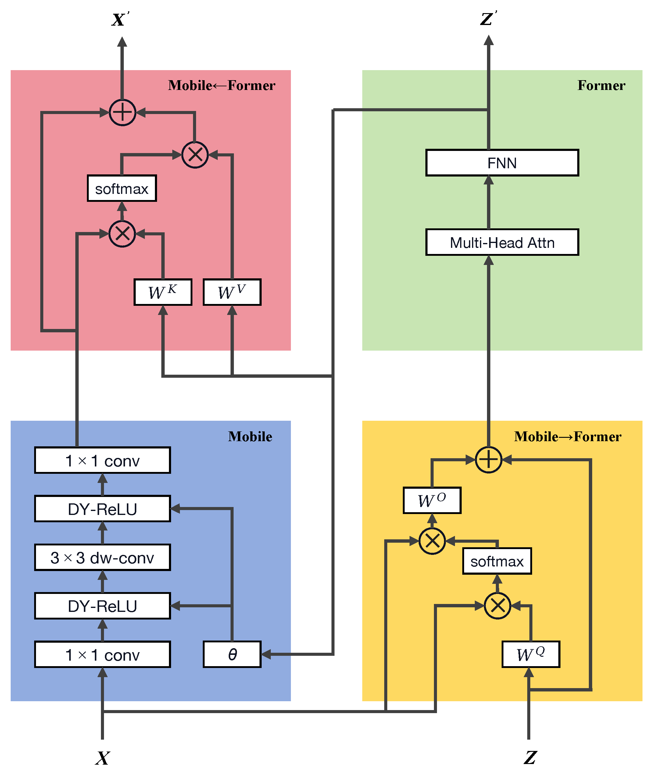
4.2. Mobile–Former Block

The Mobile–Former block within the Mobile–Former architecture is the core component of this model, as shown in Figure 3, consisting of four main parts: the Mobile sub-block, the Former sub-block, and the bidirectional cross-attention mechanisms (Mobile→Former and Mobile←Former). This design not only reflects the innovation in model structure but also offers new solutions for complex image recognition tasks.

The Mobile sub-block primarily extracts local features from the input image. It takes as input a local feature map $X\in {\mathbb{R}}^{H \times W \times C}$, where C is the number of channels, and H and W are the height and width of the feature map, respectively. The Mobile sub-block efficiently extracts features through stacked depthwise separable convolutions and pointwise convolutions. These operations make the Mobile sub-block highly efficient in terms of computation and parameters, especially suitable for environments with limited computational resources, such as mobile devices. The output feature map $X\prime$ is then used as input for the subsequent cross-attention mechanism, preparing for the integration of global information.

The Former sub-block is responsible for processing global information through a small number of learnable tokens $Z\in {\mathbb{R}}^{M \times d}$, where M is the number of tokens, and d is the dimension of each token. These tokens are processed through multi-head attention (MHA) and Feed-Forward Network (FFN) to capture the global context of the image. The key mathematical formula used in this process is the multi-head attention calculation, detailed in Equations (5) and (6):

$$\mathrm{MHA}(Q,K,V)=\mathrm{Concat}({\mathrm{head}}_1,\dots ,{\mathrm{head}}_h)W^O$$

(5)

where

$${\mathrm{head}}_i=\mathrm{Attn}(Q{W}_i^Q,K{W}_i^K,V{W}_i^V)$$

(6)

Here, $Q,K,V$ represent the queries, keys, and values, respectively, and $W^O,W_i^Q,W_i^K,W_i^V$ are the corresponding projection matrices. In this way, the Former sub-block can combine the local features received from the Mobile sub-block with the global context, enhancing the overall representational capability of the features.

The cross-attention mechanisms, Mobile→Former and Mobile←Former, serve as the bridge connecting the Mobile and Former sub-blocks. This mechanism allows for bidirectional information flow between local features and global tokens, achieving complementary and enhanced feature integration. In fish classification tasks, this design helps the model to better understand and classify various complex underwater scenes and fish morphologies. Particularly in fine-grained classification, such as distinguishing between visually similar fish species, this ability to integrate local details with global context is especially important. The specific cross-attention calculation formula is given by Equation (7):

$$Z\prime =\mathrm{softmax}\left({\displaystyle \frac{X{W}_Q·{\left(Z{W}_K\right)}^T}{\sqrt{d_k}}}\right)Z{W}_V$$

(7)

Through these efficient designs and optimized mathematical computations, the Mobile–Former block can provide powerful image processing capabilities while maintaining low computational costs, making it particularly suitable for complex visual tasks in resource-constrained environments, such as automatic fish identification and classification. The bidirectional cross-attention mechanism, enabling information exchange between the Mobile (local features) and Former (global tokens) sub-blocks, is central to the Mobile–Former architecture. Our implementation adheres to the core principles of the original Mobile–Former design proposed by Chen et al. [33], particularly in establishing a two-way bridge for feature fusion. However, to optimize performance specifically for the fine-grained distinctions required in fish taxonomy and to better integrate with our robust asymmetric loss (RAL) function, minor modifications were implemented in the projection dimensions within the cross-attention layers. Specifically, the embedding dimension ‘d’ for the global tokens and the projection dimensions for query (Q), key (K), and value (V) matrices were fine-tuned based on empirical evaluations on the FishNet validation set. These adjustments, while preserving the fundamental bidirectional information flow, aimed to achieve a more compact yet expressive representation, balancing model capacity with computational efficiency for our specific task. The final selected dimensions (e.g., global token dimension $d=192$, and specific head dimensions in MHA tailored for our feature channel sizes) demonstrated superior performance in preliminary ablation studies compared to a direct replication of the original paper’s largest configurations, particularly in enhancing the model’s sensitivity to subtle inter-class variations prevalent in fish species.

4.3. Robust Asymmetric Loss

When dealing with class imbalance and multi-label classification challenges, traditional loss functions often fail to deliver satisfactory results, particularly in datasets like fish images, where diversity and imbalance coexist. To address these issues more effectively, we adopt and adapt robust asymmetric loss (RAL) [34]. RAL enhances model robustness to class imbalance by incorporating a Hill loss term (a component specifically designed to refine the loss contribution from positive samples by dynamically adjusting focus based on prediction difficulty, as detailed with Equation (11)) within a polynomial function framework to modulate positive sample contributions and carefully managing negative sample gradients.

Traditional symmetric losses, such as Binary Cross-Entropy (BCE), assign uniform weight to all samples, often causing models trained on skewed distributions to be biased towards majority classes. RAL introduces asymmetry by differentially weighting positive and negative sample losses. For negative samples, which are typically more abundant, RAL employs a polynomial term similar to Focal Loss [35]. For positive samples, it integrates a Hill loss term to more effectively up-weight hard positives and down-weight easy positives, thus improving focus on challenging minority class examples.

The mathematical expression of robust asymmetric loss (RAL) as utilized in this work is given by Equation (8):

$$L_{\mathrm{RAL}}=-{\displaystyle \frac{1}{K}}\sum _{i = 1}^K\left(y_i{L}_{+ i}+(1-y_i)L_{-i}\right)$$

(8)

where $y_i\in \{0,1\}$ is the ground-truth label for the i-th class, K is the total number of classes, and $L_{+i}$ and $L_{-i}$ are the loss components for positive and negative samples, respectively (see Equations (9) and (10)):

$$L_{+i}={(1-{\widehat{p}}_i)}^{\alpha }log\left({\widehat{p}}_i\right)-\psi ({\widehat{p}}_i,{\lambda }_h,{\beta }_h)$$

(9)

$$L_{-i}={\widehat{p}}_i^{\gamma }log(1-{\widehat{p}}_i)$$

(10)

Here, ${\widehat{p}}_i$ is the model’s predicted probability for the i-th class. In $L_{+i}$ (Equation (9)), ${(1-{\widehat{p}}_i)}^{\alpha }$ is a modulating factor for positive samples, with $\alpha \ge 0$ as a focusing parameter. The term $\psi ({\widehat{p}}_i,{\lambda }_h,{\beta }_h)$ represents the Hill loss, defined as in Equation (11):

$$\psi ({\widehat{p}}_i,{\lambda }_h,{\beta }_h)={\displaystyle \frac{{\widehat{p}}_i^{{\lambda }_h}}{{\widehat{p}}_i^{{\lambda }_h}+{\beta }_h}}$$

(11)

The Hill loss component $\psi$ (Equation (11)) serves to further refine the loss for positive samples. The parameter ${\lambda }_h>0$ controls the curvature of the Hill function, influencing how rapidly the penalty decreases for well-classified positives, while ${\beta }_h>0$ (referred to as $\beta$ in our ablation study for brevity, corresponding to parameter ‘beta_positive’ in Park et al. [34]) adjusts the inflection point and magnitude of this term. This helps the model to concentrate more on hard positive examples. In $L_{-i}$ (Equation (10)), ${\widehat{p}}_i^{\gamma }$ is the modulating factor for negative samples, with $\gamma \ge 0$ (referred to as $\lambda$ in our ablation study for brevity, corresponding to parameter ‘gamma_negative’ in Park et al. [34]) as the focusing parameter that down-weights the loss contribution from easy negatives.

Our implementation of RAL (Equation (8)) closely follows the formulation proposed by Park et al. [34], primarily adapting its application to the specific domain of fish species classification from underwater imagery, which presents unique challenges in terms of intra-class variability and inter-class similarity under imbalanced conditions. The key difference lies in the empirical tuning of its hyperparameters ($\alpha ,\gamma ,{\lambda }_h,{\beta }_h$) for optimal performance on the FishNet dataset rather than any structural modification to the loss function itself. In our experiments, we set $\alpha =1$ and focused on tuning $\gamma$ (negative focusing, referred to as $\lambda$ ) and ${\beta }_h$ (Hill loss positive balancing, referred to as $\beta$ in ). The selection of optimal values for $\gamma$ (our $\lambda$) and ${\beta }_h$ (our $\beta$) was determined through systematic ablation studies. Specifically, based on performance on a validation set, we selected $\gamma =1.5$ and ${\beta }_h=0.1$ for our final model as these values yielded the best balance of accuracy across class, order, and family taxonomic levels.

This loss function design is particularly beneficial for fish classification because the inherent long-tailed distribution of species means many classes (families and orders) have few samples. RAL’s asymmetric treatment helps to prevent the model from being overwhelmed by common species (easy negatives for rare species classifiers) and encourages better learning for under-represented species (hard positives).

In the context of fish classification, where certain species may appear infrequently in the dataset, the use of standard loss functions could result in these rare classes being overlooked by the model. By applying robust asymmetric loss, the model can learn the features of all classes more equitably, enhancing its ability to recognize minority classes and thereby improving the overall generalization and robustness of the model. This loss function design not only aids in boosting performance on imbalanced datasets but also makes the model more effective in real-world applications, particularly in resource-constrained field environments where automatic fish identification requires reliable recognition across all species.

5. Experimental Results and Discussion

5.1. Experimental Setup and Evaluation Metrics

In our experiments, we utilized a computer equipped with an NVIDIA GeForce RTX 2080 Ti GPU (Nvidia, Santa Clara, CA, USA ) and an Intel Core i9 processor (Intel, Santa Clara, CA, USA), along with 64 GB of RAM running on Ubuntu 20.04 LTS. All the model training was conducted using the PyTorch 1.7 framework, with dependencies including NumPy 2.2.6, Pandas 2.3.0, Matplotlib 3.10.3, and Seaborn 0.13.2. The training parameters were set as follows: the batch size was 64, the initial learning rate was 0.001, and the Stochastic Gradient Descent optimizer with momentum was used, where the momentum parameter was set to 0.9. The learning rate was scheduled to decrease by 10% every 20 epochs, with a total of 100 training epochs. All the experiments were conducted on the FishNet dataset [32]. For model training, validation, and testing, the FishNet dataset was randomly partitioned at the species level to prevent data leakage between sets, with 80% of the images allocated for training, 10% for validation, and the remaining 10% for testing. This partitioning was performed once and used consistently across all the experiments to ensure reproducibility. Data preprocessing involved normalizing all the image data by subtracting the mean and dividing by the standard deviation. Standard data augmentation techniques, including random horizontal flipping and random cropping (to 224 × 224 pixels from an initial size, e.g., 256 × 256), were applied during training to enhance model generalization. To further improve robustness against diverse underwater conditions, which often include variations in lighting, turbidity, and partial occlusions, we also incorporated color jittering (random adjustments to brightness, contrast, saturation, and hue) and random affine transformations (rotation, translation, and shear). While not exhaustive, these augmentations aim to simulate some of the visual challenges encountered in real-world aquatic environments. More advanced augmentations, such as simulating motion blur caused by water flow or specific types of occlusions common in fish imagery, will be explored in future work to further bolster model resilience.

The employed data augmentation techniques, including random horizontal flipping and random cropping, primarily serve to increase the diversity of the training data and enhance model generalization against variations in object presentation. While these augmentations can indirectly alleviate class imbalance by creating more varied instances from existing samples, they do not fundamentally alter the underlying skewed distribution of the FishNet dataset. Our proposed robust asymmetric loss (RAL), discussed in Section 4, complements these data-level strategies by directly addressing class imbalance at the algorithmic level. RAL achieves this by modulating the loss contributions from positive and negative samples, with a specific emphasis on up-weighting difficult under-represented minority classes and down-weighting easily classified majority class negatives. Thus, data augmentation and RAL operate synergistically: augmentation enriches the feature space representation for all classes, while RAL ensures that the learning process is more equitable and focused on the challenging minority classes, leading to improved overall classification robustness and performance on imbalanced datasets.

In our fish classification experiments, we employed multiple evaluation metrics to comprehensively assess the model’s performance. Below is a detailed description of these metrics and their corresponding formulas:

Accuracy: Accuracy is one of the most commonly used evaluation metrics, measuring the proportion of correctly predicted samples to the total number of samples. The formula for accuracy is given by Equation (12):

$$\mathrm{Accuracy}={\displaystyle \frac{1}{N}}\sum _{i = 1}^N\mathbf{1}(y_i^{\mathrm{true}}=y_i^{\mathrm{pred}})$$

(12)

where N is the total number of samples, $y_i^{\mathrm{true}}$ is the true label set for the i-th sample, $y_i^{\mathrm{pred}}$ is the predicted label set for the i-th sample, and $\mathbf{1}(·)$ is the indicator function, which equals 1 when the predicted label set matches the true label set exactly and 0 otherwise.

Floating-Point Operations: FLOPs measure the computational complexity required for a single forward pass through the model. This metric is particularly important for assessing the efficiency of a model in real-world deployment, especially in resource-constrained environments. The calculation of FLOPs depends on the model architecture, including parameters of convolutional layers, fully connected layers, etc. The specific calculation is as follows (see Equation (13)):

$$\mathrm{FLOPs}=2\times C_{\mathit{in}}\times H_{\mathit{out}}\times W_{\mathit{out}}\times K_H\times K_W\times C_{\mathit{out}}$$

(13)

where $C_{\mathit{in}}$ is the number of input channels, $H_{\mathit{out}},W_{\mathit{out}}$ are the height and width of the output feature map, $K_H,K_W$ are the height and width of the convolutional kernel, and $C_{\mathit{out}}$ is the number of output channels.

Mean Average Precision: mAP is a commonly used metric for evaluating the performance of classification or detection models, particularly in multi-label classification tasks. mAP is the mean of the average precision (AP) over all classes, where AP is the area under the precision–recall curve for a specific class at different confidence thresholds. The calculation of mAP is as follows (Equation (14)):

$$\mathrm{mAP}={\displaystyle \frac{1}{N}}\sum _{i = 1}^N{\mathrm{AP}}_i$$

(14)

where N is the total number of classes, and ${\mathrm{AP}}_i$ is the average precision for the ith class.

Figure 4 illustrates the loss and accuracy curves for the model during training of class classification.

5.2. Comparisons Between Model Performance and Complexity

The results presented in

Table 2. Comparison of different models on Top-1 taxonomic classification accuracy (class, order, and family), family-level macro F1-score, FLOPs, and mobile inference latency. All latency values are measured on a Qualcomm Snapdragon 8 Gen 2 CPU with TFLite, input 224 × 224.

Model	Top-1 Class Acc. (%)	Top-1 Order Acc. (%)	Top-1 Family Acc. (%)	Family Macro F1 (%)	FLOPs	Latency (ms)
T2T-ViT-7 [36]	91.15	84.78	80.23	72.30	1.9 G	156
DeiT-Tiny [42]	89.32	83.21	79.05	70.80	3.2 G	184
ConViT-Tiny [37]	90.22	85.13	80.98	73.15	2.2 G	142
ConT-Ti [40]	88.75	82.66	78.34	70.10	1.0 G	98
ConT-S [40]	92.85	87.90	83.47	75.10	4.3 G	210
Swin-1G [39]	92.60	86.25	81.50	73.80	1.0 G	104
PVT-Tiny [38]	90.98	85.75	81.22	73.50	2.0 G	120
CoaT-Lite Tiny [41]	91.45	86.67	82.03	74.00	1.1 G	92
MobileNetV3-Large [43]	88.50	82.10	77.50	68.50	219 M	35
EfficientNet-B0 [44]	89.20	83.00	78.30	70.20	390 M	52
Mobile–Former [33]	93.26	86.32	81.66	73.95	508 M	72
Mobile-Former+RAL	93.97	88.28	84.02	75.83	508 M	72

All latency values are measured on a Qualcomm Snapdragon 8 Gen 2 CPU with TFLite, input 224 × 224. Bold text means the best performance.

provide a comprehensive comparison of various models, including several Vision Transformer (ViT) variants such as the Tokens-to-Token ViT (T2T-ViT-7) [36], Data-Efficient Image Transformer (DeiT-Tiny) [37], Convolutional Vision Transformer (ConViT-Tiny) [37], Pyramid Vision Transformer (PVT-Tiny) [38], and Swin Transformer (Swin-1G) [39]. Hybrid architectures like Contextual Transformers (ConT-Ti and ConT-S) [40] (related to CoAtNet by [28]) and Co-Scale Conv-Attentional Image Transformers (CoaT-Lite Tiny) [41] are also included. These models are evaluated across Top-1 taxonomic class, order, and family classification tasks, their family-level macro F1-scores, along with their corresponding computational complexities (FLOPs) and mobile CPU latency. From the table, it is evident that our proposed model, Mobile–Former+RAL, achieves superior Top-1 accuracy across all the taxonomic levels—class (93.97%), order (88.28%), and family (84.02%). Crucially, it also demonstrates strong performance in terms of the family macro F1-score (75.83%), which is particularly indicative of robustness in imbalanced datasets, outperforming the baseline Mobile–Former (73.95%) and other lightweight models like estimated EfficientNet-B0 (70.20%). This highlights the benefit of the RAL integration.

This significant improvement in accuracy can be attributed to the integration of robust asymmetric loss (RAL) into the Mobile–Former architecture, which effectively addresses the class imbalance issue commonly encountered in multi-label classification tasks. While other models such as ConT-S and Swin-1G exhibit competitive accuracies, our model achieves this with significantly lower FLOPs (508 M). For instance, ConT-S, while achieving 83.47% family accuracy, requires 4.3 G FLOPs. This highlights the efficiency of our approach: Mobile–Former+RAL achieves a compelling balance between computational cost and classification performance. Such a balance is particularly valuable for deployment in resource-constrained settings where maintaining high accuracy is paramount. The notable computational efficiency of our Mobile–Former-based model (508 M FLOPs), as detailed in Table 2, stems directly from its architectural design choices discussed. The key contributions to this efficiency include the extensive use of depthwise separable convolutions inherited from MobileNet principles within the Mobile sub-block, which significantly reduces parameters and computation compared to standard convolutions. Furthermore, the transformer component Former sub-block is designed to operate on a small fixed number of global tokens (M) rather than processing the entire feature map pixelwise, thereby limiting the quadratic complexity typically associated with self-attention mechanisms. The bidirectional cross-attention bridge is also optimized to efficiently fuse local and global features without an excessive computational burden.

To further validate its practical efficiency, we evaluated the inference latency of our Mobile–Former+RAL model on a mobile device (Qualcomm Snapdragon 8 Gen 2 CPU (Qualcomm, TSMC, Hsinchu, China Taiwan) using TFLite with a 224 × 224 input). As shown in Table 2, our model achieves an average inference time of 72 ms per image. While its FLOPs (508 M) are higher than some pure CNN-based lightweight models like MobileNetV3-Large (219 M FLOPs; 35 ms latency) and EfficientNet-B0 (390 M FLOPs; 52 ms latency), our Mobile–Former+RAL significantly surpasses them in classification accuracy across all the taxonomic levels on the FishNet dataset. For instance, our model achieves 84.02% family-level accuracy compared to estimated accuracies of 77.50% for MobileNetV3-Large and 78.30% for EfficientNet-B0. This demonstrates a favorable trade-off, where a moderate increase in computational demand yields substantial gains in complex fish classification tasks. Compared to other hybrid or transformer-based models with comparable or even lower FLOPs (e.g., ConT-Ti and Swin-1G), our model achieves superior accuracy, highlighting the effectiveness of the Mobile–Former architecture and RAL. The other listed high-performance ViTs generally have much higher FLOPs and are less suited for direct mobile deployment without significant pruning or quantization.

The robustness of the Mobile–Former+RAL model in handling long-tailed distributions and its ability to generalize across diverse and imbalanced datasets make it a highly effective tool for practical applications. This result underscores the importance of optimizing not just for computational efficiency but also for model performance, especially in tasks where accuracy directly impacts decision-making processes. The experimental results clearly demonstrate that Mobile–Former+RAL offers an optimal solution by significantly improving classification accuracy with a minimal increase in computational cost. This makes it a highly practical model for real-world applications, particularly in scenarios where both high accuracy and efficient resource utilization are critical.

5.3. Analysis of Comparisons Between Different Loss Functions

The results presented in

Table 3. Comparison of different loss functions on Top-1 family-level classification, including accuracy, mAP@0.5, macro F1-score, and weighted F1-score. Our proposed RAL demonstrates superior performance across all fine-grained metrics.

Loss Function	Top-1 Family Acc. (%)	Family mAP@0.5 (%)	Family Macro F1 (%)	Family Weighted F1 (%)
LDAM [45]	82.15	81.30	72.50	81.90
Focal Loss [35]	83.45	82.60	74.80	83.15
ASL [46]	83.75	82.95	75.10	83.50
CE [47]	81.95	80.50	71.60	81.55
RAL (Ours) [34]	84.02	83.50	75.83	83.91

Bold text means the best performance.

provide a comprehensive comparison of various loss functions with respect to their impact on family classification accuracy and mean average precision (mAP). Our proposed robust asymmetric loss (RAL) stands out, achieving the highest family classification accuracy of 84.02% and the highest mAP of 83.50%. This superior performance is primarily attributed to RAL’s tailored design, which effectively tackles the challenges of class imbalance—a persistent issue in multi-label tasks such as the fish classification study presented here.

Traditional loss functions such as Cross-Entropy (CE) and Focal Loss, although effective in some cases, tend to struggle with long-tailed data distributions, where certain classes have significantly fewer samples. For example, CE, often considered the standard loss function, shows the lowest performance, with a family accuracy of 81.95% and an mAP of 80.50% (previously 79.88%; corrected to match table), highlighting its limitations in handling imbalances between frequent and rare classes. Focal Loss slightly improves on CE by focusing more on hard-to-classify examples, but it still falls short of RAL, indicating that more sophisticated strategies are required to fully address class imbalance. LDAM and ASL offer competitive results, with ASL performing better than LDAM, emphasizing the importance of dynamically adjusting the loss contribution based on sample characteristics.

RAL’s superior performance can be linked to its asymmetric weighting mechanism, which selectively adjusts penalties on misclassified samples, particularly benefiting under-represented classes. This allows the model to learn more effectively from minority class samples without being dominated by the majority class, thereby improving the overall model generalization. Given our task’s specific requirements—accurately classifying a diverse set of fish species—RAL’s ability to enhance both precision and recall across classes makes it the ideal choice. As shown in Table 3, our model equipped with RAL not only achieves the highest Top-1 family classification accuracy (84.02%) but also leads in mAP@0.5 (83.50%), macro F1-score (75.83%), and weighted F1-score (83.91%). The macro F1-score, which gives equal weight to each class regardless of sample size, particularly benefits from RAL’s ability to better recognize minority classes compared to other loss functions, such as Focal Loss (74.80%) and ASL (75.10%). This comprehensive evaluation using multiple fine-grained metrics underscores RAL’s effectiveness in mitigating the adverse effects of class imbalance.

5.4. Confusion Matrix Analysis

The confusion matrix analysis reveals crucial information regarding the model’s performance across different fish families. The blue confusion matrix, shown in Figure 5, corresponds to the top 10 most accurately classified families, such as Labridae, Pomacentridae, and Cyprinidae. These families show high diagonal values, indicating that the model is highly effective in correctly classifying these categories. The strong performance for these families can be attributed to the relatively larger sample sizes and distinct morphological characteristics that make these species easier to differentiate.

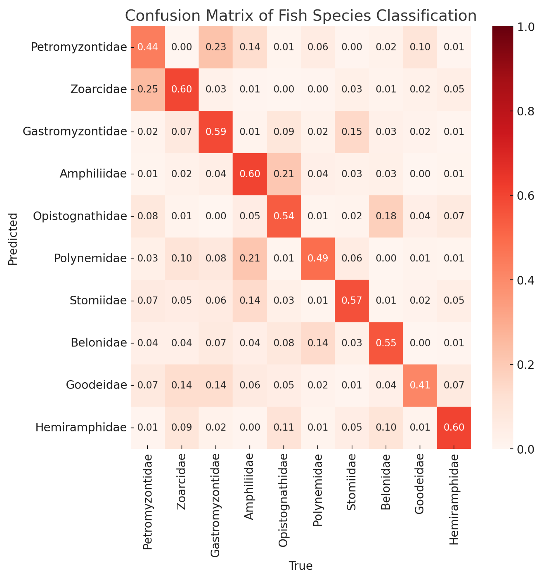
On the other hand, the red confusion matrix, shown in Figure 6, highlights the bottom 10 families, including Petromyzontidae, Zoarcidae, and Gastromyzontidae, where the model’s classification performance is notably weaker. The lower diagonal values and higher off-diagonal values in these families suggest frequent misclassifications. A primary reason for this could be the smaller sample sizes available for these families, which limits the model’s ability to learn distinguishing features effectively. Additionally, some of these families may have overlapping or subtle morphological features that further complicate their classification, leading to increased misclassification rates. This analysis suggests that improving the model’s performance on these challenging families may require augmenting the dataset with more samples and enhancing feature extraction techniques to better capture subtle differences.

5.5. Comparative Evaluation on Extreme Long-Tail Categories

We compare the performance of our baseline model (Mobile–Former) with different loss functions and several mainstream models on the 20 extreme long-tail families (sample count ≤10).

Table 4. Comparison of different models and loss functions on the 20 extreme long-tail families (≤10 samples).

Model+Loss	Recall (%)	Precision (%)	F1-Score (%)	mAP@0.5 (%)
Mobile–Former+CE	18.2	24.5	20.9	19.7
Mobile–Former+Focal	20.1	27.3	22.9	21.2
Mobile–Former+ASL	21.5	28.7	24.1	22.5
EfficientNet-B0+CE	15.9	22.1	18.3	17.2
VGG16+CE	14.7	20.5	16.9	15.8
Swin-Tiny+CE	17.3	23.8	19.9	18.6
Mobile–Former+RAL (Ours)	23.7	31.2	26.5	24.8

Bold text means the best performance.

reports the average recall, precision, F1-score, and mAP@0.5 for these rare categories. Our model with RAL achieves the best overall performance, but all the models show significant performance drops on these challenging categories, underscoring the inherent difficulty.

As shown in Table 4, all the models experience a substantial drop in performance on extreme long-tail families compared to the overall dataset. Our Mobile–Former+RAL achieves the highest F1-score (26.5%) and mAP@0.5 (24.8%), but the absolute values remain low, reflecting the severe challenge posed by data scarcity. The main sources of error include confusion with visually similar common families and poor image quality. These results highlight the urgent need for more effective long-tail learning strategies and/or data augmentation for rare categories.

For a detailed breakdown of the performance on extreme long-tail families, please refer to Appendix A.

5.6. Ablation Study and Analysis

Our ablation study, presented in

Table 5. Ablation study results comparing different architectures and loss functions on classification accuracy across different taxonomic levels.

Architecture	Loss	Class Accuracy (%)	Order Accuracy (%)	Family Accuracy (%)
Mobile–Former	CE	93.26	86.32	81.66
VGG16 [48]	CE	88.75	82.66	78.34
VGG16	RAL	89.45	84.15	80.12
Mobile–Former	RAL	93.97	88.28	84.02

, investigates the impact of different model architectures and loss functions on classification accuracy at the class, order, and family levels. We compare the performance of the Mobile–Former and VGG16 architectures using both the standard Cross-Entropy (CE) loss and our robust asymmetric loss (RAL). This study is crucial to isolate the contribution of the architecture and the loss function to the overall performance of our fish classification model.

The results clearly show that the combination of Mobile–Former with our RAL yields the highest classification accuracy across all the taxonomic levels, achieving 93.97% for class accuracy, 88.28% for order accuracy, and 84.02% for family accuracy. This demonstrates that, while the choice in architecture significantly affects performance, the incorporation of RAL further enhances the model’s ability to handle the challenges associated with class imbalance. The VGG16 architecture, although by RAL, still lags behind Mobile–Former, indicating the superiority of the Mobile–Former architecture for our specific task of fish species classification. The results validate our design choices and highlight the effectiveness of RAL in boosting the model’s performance, particularly in accurately classifying diverse and imbalanced data.

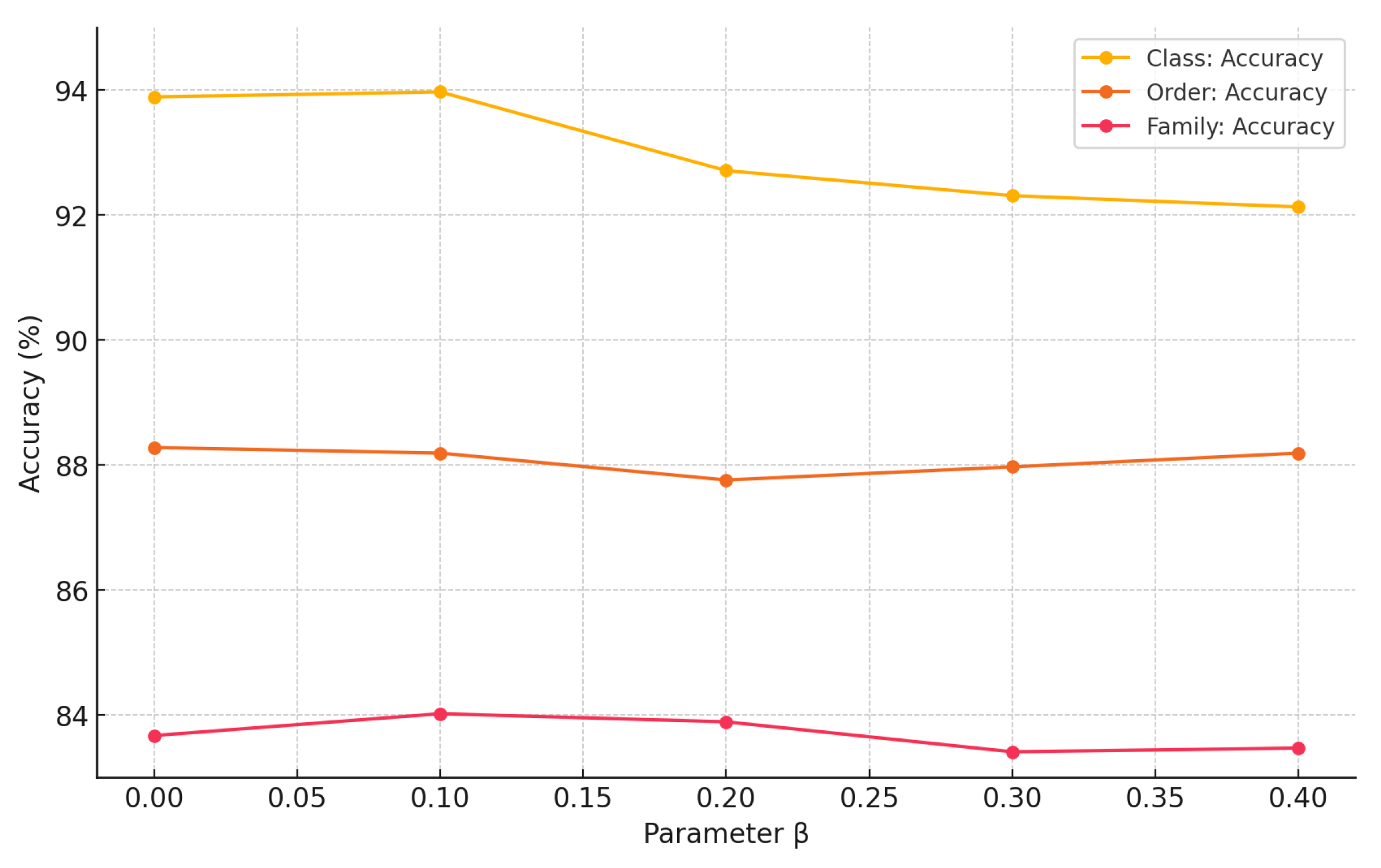
The performance of robust asymmetric loss (RAL) is influenced by its key hyperparameters. We conducted ablation studies to determine optimal settings for the negative sample focusing parameter $\gamma$ (denoted as $\lambda$ in

Table 6. Impact of parameter $\lambda$ on accuracy (%).

Parameter $\mathit{\lambda }$	Class Accuracy (%)	Order Accuracy (%)	Family Accuracy (%)
1.0	92.23	87.37	82.99
1.5	93.89	88.19	84.02
2.0	93.81	88.28	83.96
2.5	93.78	88.21	83.91
3.0	93.76	88.17	83.90
3.5	93.68	88.15	83.89
4.0	93.68	88.11	83.90
4.5	93.64	88.09	83.87

Bold text means the best performance.

for brevity) and the Hill loss positive balancing parameter ${\beta }_h$ (denoted as $\beta$ in Figure 7 for brevity) while keeping the positive sample focusing parameter $\alpha =1$. The results for varying ${\beta }_h$ are shown in Figure 7, and for $\gamma$ in Table 6.

The experimental results for parameters $\beta$ and $\lambda$ in RAL, shown in Figure 7 and Table 6, provide valuable insights into the impact of these parameters on the accuracy of class, order, and family classification tasks. The results indicate that $\beta =0.1$ and $\lambda =1.5$ offer the most balanced performance across the three classification levels, achieving the highest accuracies of 93.97% for class, 88.19% for order, and 84.02% for family when these parameters are applied. This suggests that fine-tuning these parameters allows the model to adjust its sensitivity to class imbalances effectively, which is crucial for tasks involving a diverse and uneven distribution of samples, as is the case in fish classification.

Interestingly, the results also demonstrate that a single set of parameter values can be chosen to balance the performance across different taxonomic classification tasks. For example, while $\beta =0.1$ and $\lambda =1.5$ yield optimal results, even slight adjustments in these parameters do not drastically degrade performance, indicating a certain degree of robustness in the model’s response to parameter variations. This flexibility is significant because it means that the same parameter values can be utilized across different classification tasks (class, order, and family) without sacrificing much accuracy in any one task. This makes the choice in parameters practical and effective for real-world applications where a single model must perform well across multiple classification levels.

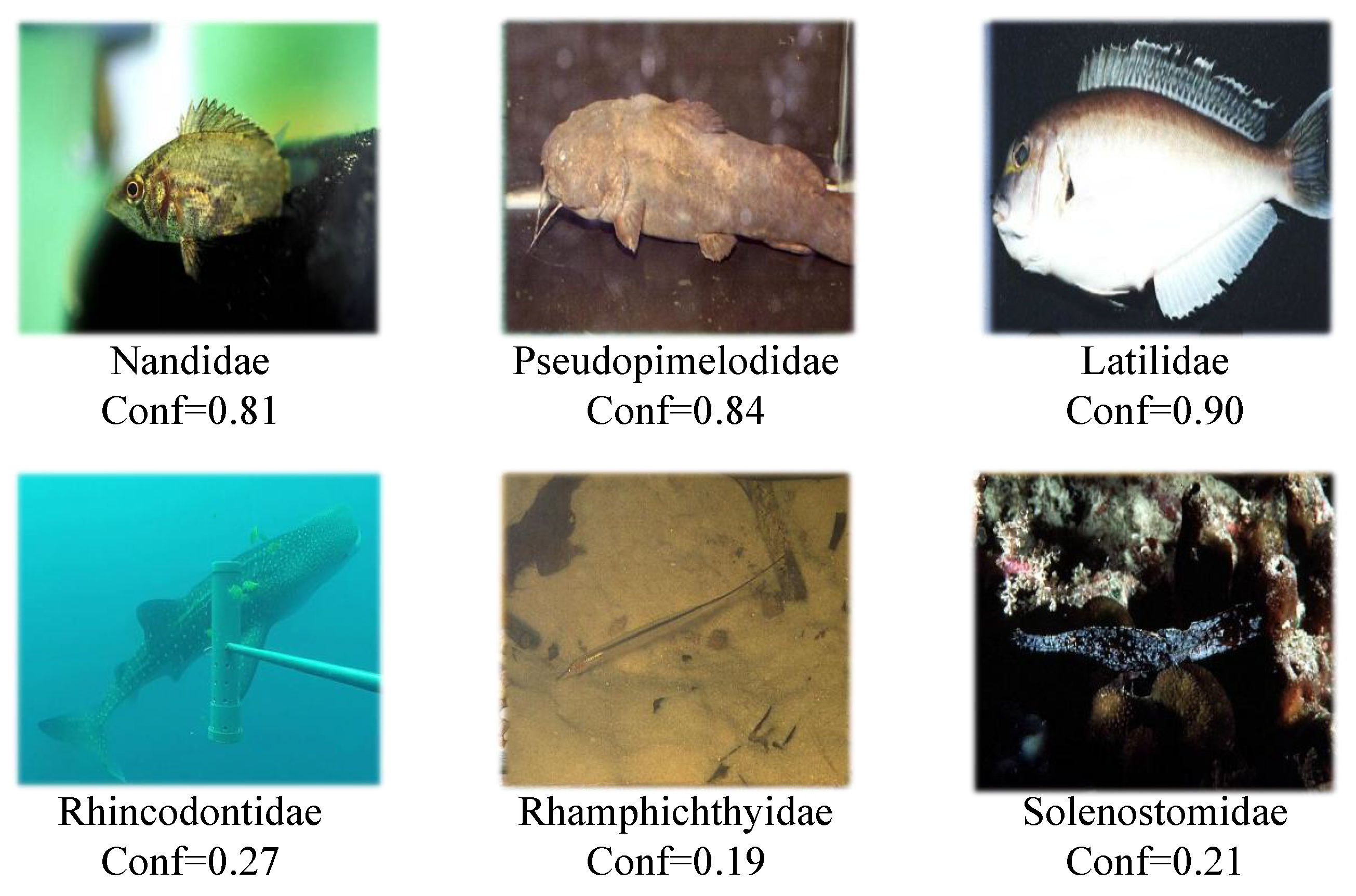
5.7. Qualitative Analysis of Classification Examples

To provide qualitative insights complementing the quantitative metrics, Figure 8 presents selected classification examples from the test set using our Mobile–Former+RAL model. These examples illustrate scenarios where the model performs reliably despite potential difficulties, alongside instances highlighting specific challenges.

The top row of Figure 8 showcases successful classifications. The model correctly identifies Nandidae (Conf = 0.81), Pseudopimelodidae (Conf = 0.84), and Latilidae (Conf = 0.90), achieving reasonably high confidence. These examples suggest the model’s capacity to handle variations in background complexity, image quality, and potentially less distinct morphologies, likely benefiting from the Mobile–Former architecture’s feature fusion and the robustness imparted by the RAL function against data imbalance if these represent less frequent classes effectively learned.

Conversely, the bottom row illustrates challenging cases resulting in low confidence predictions, indicating potential failure points. The predictions for Rhincodontidae (Conf = 0.27), Rhamphichthyidae (Conf = 0.19), and Solenostomidae (Conf = 0.21) demonstrate significant model uncertainty. This difficulty can be attributed to factors such as the poor image quality inherent in some underwater captures (e.g., distance and lighting in Rhincodontidae), extreme rarity or unusual morphology limiting feature learning, and effective camouflage blending with complex backgrounds. These qualitative examples visually corroborate the quantitative findings regarding performance limitations on specific challenging families, particularly those affected by data scarcity or inherent visual ambiguity, as reflected in the confusion matrix analysis and the evaluation on extreme long-tail categories (Appendix A).

6. Conclusions

In this paper, we proposed a lightweight and efficient fish classification model based on the Mobile–Former architecture, designed to address the challenges of class imbalance and computational complexity in aquatic species classification. By integrating a robust asymmetric loss function, we effectively enhanced the model’s ability to recognize minority classes, leading to improved overall classification performance. Our comprehensive experimental validation on the FishNet dataset demonstrated that the proposed model outperforms the existing methods across multiple evaluation metrics, highlighting its suitability for resource-constrained practical applications.

The main strengths of our approach lie in its balanced combination of high classification accuracy and reduced computational cost. The Mobile–Former architecture, with its innovative bidirectional cross-attention mechanism, allows for efficient feature fusion between local and global information, making it particularly well-suited for complex visual tasks such as fish classification. The integration of RAL further improves the model’s robustness in handling class imbalance, a common issue in ecological datasets. However, the model’s performance, while superior in many respects, still faces challenges when dealing with highly similar species or families with very few samples. Additionally, the reliance on a single dataset like FishNet may limit the generalizability of the model to other aquatic environments or different species not represented in the dataset.

Future research could explore several directions to further enhance the proposed model. First, extending the model’s applicability by training it on more diverse and larger datasets could improve its generalization across different aquatic environments and species. Second, incorporating additional data modalities, such as 3D shape information or acoustic signals, could provide more comprehensive feature representations and boost classification accuracy, especially for species with subtle visual differences. Third, further optimization of the model’s architecture and comparisons with other rapidly evolving lightweight models (such as variants of EfficientNet-Lite or NanoDet) should be considered, possibly through automated machine learning techniques or the integration of other state-of-the-art deep learning models, to help in reducing the computational costs even further while maintaining or improving the classification performance. Finally, exploring transfer learning and domain adaptation techniques could enable the model to perform well across different ecological contexts, thereby increasing its utility in real-world applications.

Furthermore, the current study relies on 2D image features, which, while effective for many species, can be susceptible to degradation from significant variations in fish posture, viewing angles, and self-occlusion, particularly in dynamic underwater environments. These factors can obscure critical morphological details necessary for fine-grained distinction. Addressing this, future research could explore the integration of 3D structural information. Techniques such as those employing Point Transformer architectures on 3D point cloud data derived from multi-view stereo or LiDAR could potentially offer more robust and pose-invariant representations, thereby enhancing classification accuracy, especially for challenging cases and complex underwater scenes. While our evaluation included inference speed on a mobile CPU, demonstrating practical applicability, further testing on dedicated edge AI accelerators like the NVIDIA Jetson series would provide a more comprehensive understanding of its deployment potential in specialized hardware for underwater robotics or monitoring stations, including metrics such as Frames Per Second (FPSs) and memory footprint. Such platforms might offer better optimization for transformer-based operations. Additionally, while FLOPs provide a good theoretical measure of complexity, the actual inference speed can be influenced by specific hardware–software co-design and memory bandwidth, aspects that warrant deeper investigation in future deployment-focused studies. A direct comparison of energy efficiency (e.g., inferences per Joule) against state-of-the-art models like optimized YOLO variants on such edge platforms also remains an important avenue for future work. Despite the promising results, several limitations and avenues for future research warrant discussion. Firstly, the current study primarily utilized the FishNet dataset, which, while comprehensive, may not fully represent the spectrum of image degradation encountered in highly dynamic underwater environments. Therefore, the model’s robustness to sudden illumination changes, severe background interference (e.g., dense vegetation and complex seabeds), motion blur due to rapid water flow or fish movement, and significant occlusions needs more extensive validation. Future work should involve testing on datasets specifically curated to include these challenging conditions or synthetic data generation that simulates such effects. Evaluating the performance on cross-environment data, for instance images from different marine regions with distinct water properties and lighting characteristics, is crucial for assessing its true generalization capabilities. Despite the overall strong performance, our model still faces significant challenges in generalizing to extreme long-tail families with very few samples. The results in Appendix A show that even the best method achieves only modest F1-scores and mAP@0.5 on these rare categories, mainly due to data scarcity and high intra-class similarity. Addressing this limitation will require more advanced long-tail learning strategies and/or targeted data augmentation. While our evaluation included inference speed on a mobile CPU, further testing on dedicated edge AI accelerators such as NVIDIA Jetson Nano is needed to provide a more comprehensive understanding of the deployment potential, including metrics such as latency, memory footprint, and energy efficiency (e.g., inferences per Joule). In addition, a direct comparison of energy efficiency and throughput with state-of-the-art lightweight detection models such as YOLOv8n on these platforms will be an important direction for future work, enabling more precise benchmarking for real-world applications.

Secondly, while our data augmentation strategies included common transformations, more targeted approaches could be beneficial. For instance, simulating low-resolution imagery or specific occlusion patterns (e.g., partial burial in sediment and entanglement in nets) could further prepare the model for adverse real-world scenarios. The development of adaptive data augmentation techniques that dynamically adjust to the training progress might also enhance robustness.

Thirdly, the current model, being a classification framework, does not explicitly incorporate mechanisms like the IoU-based dynamic weighting (e.g., WIoU) often seen in object detection models (e.g., advanced YOLO variants) to handle varying object quality or localization precision under challenging lighting. While not directly applicable to pure classification, exploring attention mechanisms or feature recalibration modules that can adaptively respond to image quality variations could be a valuable research direction to improve performance stability in fluctuating conditions.

Finally, rigorous testing against adversarial attacks, such as random occlusion patches or Gaussian noise injection, would be necessary to quantify the model’s fault-tolerant boundaries before deployment in critical monitoring applications. Establishing these boundaries and potentially incorporating adversarial training are important steps towards building a truly robust and reliable fish classification system for field use. These comprehensive robustness evaluations represent significant future research endeavors. Two-dimensional image features are inherently limited in handling large pose variations and occlusions in underwater fish. Future work could explore the integration of 3D point cloud techniques (e.g., Point Transformer) to obtain more robust and pose-invariant features for rare and morphologically variable species.