Spatio-Temporal Attention-Based Deep Learning for Smart Grid Demand Prediction

Abstract

Accurate short-term load forecasting is vital for the reliable and efficient operation of smart grids, particularly under the uncertainty introduced by variable renewable energy sources (RESs) such as solar and wind. This study introduces ST-CALNet, a novel hybrid deep learning framework that integrates convolutional neural networks (CNNs) with an Attentive Long Short-Term Memory (LSTM) network to enhance forecasting performance in renewable-integrated smart grids. The CNN component captures spatial dependencies from multivariate inputs, comprising meteorological variables and generation data, while the LSTM module models temporal correlations in historical load patterns. An embedded attention mechanism dynamically weights input sequences, enabling the model to prioritise the most influential time steps, thereby improving its interpretability and robustness during demand fluctuations. ST-CALNet was trained and evaluated using real-world datasets that include electricity consumption, solar photovoltaic (PV) output, and wind generation. Experimental evaluation demonstrated that the model achieved a mean absolute error (MAE) of 0.0494, root mean squared error (RMSE) of 0.0832, and a coefficient of determination (R²) of 0.4376 for electricity demand forecasting. For PV and wind generation, the model attained MAE values of 0.0134 and 0.0141, respectively. Comparative analysis against baseline models confirmed ST-CALNet’s superior predictive accuracy, particularly in minimising absolute and percentage-based errors. Temporal and regime-based error analysis validated the model’s resilience under high-variability conditions such as peak load periods, while visualisation of attention scores offered insights into the model’s temporal focus. These findings underscore the potential of ST-CALNet for deployment in intelligent energy systems, supporting more adaptive, transparent, and dependable forecasting within smart grid infrastructures.

1. Introduction

Accurate short-term load forecasting (STLF) is a cornerstone for the reliable, efficient, and economically viable operation of modern smart grids. With the escalating integration of renewable energy sources (RESs), such as solar photovoltaic (PV) and wind power, the spatio-temporal variability and intermittency of supply have significantly increased [1,2]. These fluctuations introduce non-linear and non-stationary patterns into load profiles, challenging conventional prediction frameworks and demanding more adaptive and robust forecasting methodologies. The inherent unpredictability of RESs, particularly during peak load hours or abrupt meteorological changes, must be precisely balanced against consumer demand to avoid grid instabilities, frequency deviations, and resource dispatch inefficiencies [3,4,5]. Moreover, high-resolution STLF is becoming indispensable for demand response optimisation, microgrid coordination, and ancillary service scheduling in deregulated energy markets [6,7,8]. In this context, enhancing the accuracy and resilience of load forecasting models is not merely a computational task, but also a systemic necessity for operational continuity and cost-effective grid management.

Conventional forecasting techniques, including autoregressive integrated moving average (ARIMA), support vector regression (SVR), and multilayer perceptrons (MLPs), have historically been used for short-term load prediction due to their interpretability and low computational cost [6,9,10,11]. However, these models are fundamentally constrained in their ability to capture the complex, non-linear, and non-stationary dynamics characterising modern power systems, particularly under the influence of distributed RESs and prosumer behaviour [9,12,13,14]. ARIMA-based models assume linear dependencies and are sensitive to missing or noisy data, while SVR and MLPs often require extensive feature engineering and fail to generalise across time-dependent regimes. Most of these classical approaches depend on stationary signal assumptions and cannot adequately account for temporal variation introduced by weather anomalies, behavioural shifts, or demand-side flexibility mechanisms [15,16,17,18]. Consequently, their performance deteriorates in real-world conditions marked by frequent structural changes and intermittent renewable output, motivating the adoption of more flexible and data-driven alternatives.

Deep learning (DL) models have emerged as powerful alternatives to traditional forecasting techniques, primarily due to their ability to autonomously extract hierarchical features from raw, high-dimensional time series data [19,20,21,22]. Unlike statistical models, which depend heavily on manual feature engineering, DL models are capable of learning both local and global patterns in data across multiple layers of abstraction. Convolutional neural networks (CNNs) [23], though developed initially for visual pattern recognition, have been successfully adapted to load forecasting tasks for their ability to extract spatial correlations from structured multivariate inputs, such as temperature, humidity, solar irradiance, and historical consumption data [1,4,24,25,26]. Their weight-sharing architecture and local receptive fields make them especially suitable for identifying periodic or location-specific demand patterns. Recurrent neural networks (RNNs) [27], in contrast, are explicitly designed for modelling temporal dependencies in sequential data and have been widely applied across domains such as speech recognition, machine translation, and financial time series forecasting. Long Short-Term Memory (LSTM) and Gated Recurrent Unit (GRU) variants are particularly effective at capturing long-range temporal correlations while mitigating issues related to vanishing gradients [3,28,29]. This makes them highly suitable for load forecasting tasks, where historical trends, seasonal cycles, and abrupt demand shifts must all be accounted for within a single predictive framework.

Among recurrent models, LSTM networks have been widely adopted in STLF applications [30,31,32,33,34]. Their gated architecture effectively addresses vanishing gradient issues and facilitates learning from long-term temporal dependencies. By selectively retaining or discarding historical information through input, forget, and output gates, LSTM networks enable the model to capture recurring seasonal trends and demand fluctuations across daily and weekly cycles [11,35]. However, a major limitation of vanilla LSTM architectures lies in their uniform treatment of all past time steps during sequence encoding. This assumption neglects the fact that certain time intervals—such as recent spikes or context-specific events—may have a disproportionately stronger influence on future load trajectories, especially under volatile renewable conditions.

To address this limitation, attention mechanisms have been integrated into LSTM-based frameworks, allowing the model to compute dynamic weight coefficients that highlight the most contextually relevant time steps in the input sequence [6,36,37]. These mechanisms act as soft aligners, guiding the model’s focus toward historically influential data points while diminishing the impact of redundant or less informative signals. For instance, attention-based encoder–decoder architectures have demonstrated superior performance in both single-step and multi-step STLF tasks, enhancing models’ interpretability and robustness to input noise [4,29,38]. Moreover, recent approaches combining attention with bidirectional LSTM (BiLSTM) structures have further refined temporal sensitivity by capturing dependencies in both forward and backward directions, offering more holistic representations of load dynamics [6,39,40].

In parallel, hybrid DL architectures that combine CNNs, LSTM networks, and attention mechanisms have emerged as state-of-the-art solutions for short-term load forecasting. These models leverage the complementary strengths of CNNs in spatial feature extraction, LSTMs in temporal sequence modelling, and attention layers in selective focus, thereby capturing complex spatial–temporal dependencies within multivariate power system data [1,35]. Such hybrid frameworks have consistently demonstrated superior performance in scenarios characterised by high variability and uncertainty, including abrupt changes in consumption patterns and fluctuations in renewable energy input.

Recent advancements have further expanded this modelling paradigm by incorporating graph-based representations and transformer mechanisms. Graph neural networks (GNNs) offer a principled approach to modelling the relational structure of energy systems, capturing nodal interdependencies among loads, substations, and distributed generators within smart grids [41]. Meanwhile, transformer-based models—initially developed for natural language processing—have been adapted to power systems for their ability to model long-range temporal dependencies without recurrence, offering scalability and parallelism advantages over conventional RNN architectures [29,42].

To establish a more comprehensive performance evaluation, recent state-of-the-art DL architectures should be included in the baseline comparisons. Transformer-based models have gained prominence for their ability to model long-range temporal dependencies without relying on sequential operations. These models utilise multi-head self-attention mechanisms, which have shown high scalability and effectiveness in various sequence modelling tasks, including time-series forecasting for energy systems [43]. Moreover, hybrid CNN-BiLSTM-Attention networks have emerged as powerful frameworks by integrating spatial and bi-directional temporal learning. Jiao et al. proposed such a model for wind power forecasting and demonstrated improved performance under volatile conditions, highlighting the synergy of spatial encoding and selective temporal focus [44]. Additionally, GNNs represent a significant advancement for load forecasting in spatially distributed systems. By modelling the grid as a graph of interconnected nodes (e.g., households, substations), GNNs effectively capture structural relationships and spatial–temporal interactions, as evidenced in recent studies on smart city applications [45]. Including these models in benchmark analyses will enhance the credibility and competitiveness of the proposed ST-CALNet framework.

Despite these technological advancements, several persistent challenges remain. Chief among them is the trade-off between predictive accuracy and interpretability, while complex hybrid models often deliver high aggregate performance metrics, they may fail to generalise across diverse operational regimes such as peak-hour congestion, low-demand overnight periods, or intervals dominated by intermittent renewable generation. Moreover, many existing studies report average errors over extended horizons, thereby obscuring granular insights into time-of-day or context-specific forecasting performance. This lack of diagnostic resolution limits the operational utility of these models in real-time grid applications where dynamic responsiveness and interpretability are paramount [8,14].

To address these gaps, this study introduces ST-CALNet, a novel hybrid DL model that combines CNN-based spatial feature extraction, LSTM-based temporal modelling, and an attention mechanism for interpretability. The model is trained and evaluated on real-world datasets comprising electricity demand, PV output, and wind generation data. Comparative performance is benchmarked against traditional and DL baselines using MAE, RMSE, MAPE, and $R^2$ metrics. Additionally, attention maps and regime-specific error diagnostics provide new insights into model behaviour, positioning ST-CALNet as a reliable and explainable forecasting tool for renewable-integrated smart grids.

1.1. Primary Applications of ST-CALNet

The proposed ST-CALNet framework is tailored for intelligent energy forecasting in renewable-integrated smart grids and supports several key operational use cases:

• Short-term load forecasting in dynamic environments: ST-CALNet enables highly accurate short-term electricity demand predictions in environments influenced by variable renewable generation, such as solar and wind. This facilitates real-time grid balancing, unit commitment, and contingency planning.
• Demand response and load shifting: by predicting near-future consumption trends, the model enables utilities and energy providers to execute effective demand response strategies. This includes identifying load curtailment opportunities and optimising time-of-use tariffs.
• Microgrid and DER integration: many existing methods for microgrid energy management systems (EMS), such as Refs. [46,47,48,49,50,51], assume prior knowledge of energy demand and generation profiles. Therefore, accurate forecasting of these profiles significantly enhances EMS performance. The model supports microgrid energy management systems by forecasting local demand alongside distributed generation inputs, thereby enhancing autonomy and reducing dependency on centralised supply.
• Resilience analysis under renewable variability: ST-CALNet’s attention mechanism and temporal diagnostics provide analytical insights into how renewable intermittency affects load predictability, enabling more informed infrastructure planning and resource allocation.

1.2. Key Contributions of This Study

This study introduces a novel hybrid deep learning architecture, ST-CALNet, that is specifically designed for short-term load forecasting in smart grids with high penetration of RESs. The contributions of this work can be summarised as follows:

• Hybrid spatio-temporal modelling: unlike conventional DL models that apply CNN or LSTM components independently, ST-CALNet tightly integrates CNNs for spatial feature extraction, LSTMs for sequential modelling, and a learnable attention mechanism within a residual framework. This fusion enables more nuanced temporal learning while preserving spatial interdependencies across multivariate inputs (e.g., consumption, PV, wind).
• Embedded residual attention mechanism: the model introduces an internal attention module between stacked LSTM layers, augmented by residual connections and layer normalisation. This configuration enhances gradient stability and interpretability, distinguishing ST-CALNet from traditional attention-based encoder-–decoder or BiLSTM models.
• Improved interpretability: attention scores are visualised and analysed to reveal the temporal focus of the model. This offers practical insights into time-dependent behaviours such as peak-hour forecasting sensitivity, an aspect that is often under-reported in similar hybrid DL models.
• Temporal regime-based evaluation: beyond conventional metrics such as MAE and RMSE, this study performs a fine-grained error analysis across different temporal regimes (e.g., peak vs. off-peak, weekday vs. weekend). This highlights when and why forecasting accuracy varies, offering a diagnostic depth that is absent from many prior studies.
• Real-world deployment relevance: the model is trained on realistic microgrid data and evaluated in terms of both performance and explainability, providing a proof of the concept for deployment in decentralised grid environments.

In comparison to prior studies (e.g., [4,6,31,38]), ST-CALNet distinguishes itself through its layered attention residual mechanism, its focus on interpretability, and its application of regime-specific error analytics. Together, these contributions represent a meaningful advancement towards transparent and reliable load forecasting in data-rich, renewable-integrated smart grids.

The remainder of this paper is organised as follows. Section 2 outlines the proposed methodology, including data preprocessing, model architecture, attention mechanism, and evaluation metrics. Additionally, this section outlines the experimental setup, the datasets used, and the details of the implementation. Section 3 and Section 4 present the results and discussion of the study, including performance comparisons, error analysis, and attention visualisations. Finally, Section 5 concludes the paper with a summary of findings, practical implications, and suggestions for future research.

2. Methodology

This section describes the end-to-end methodology of the proposed ST-CALNet model, including data preprocessing, spatio-temporal sequence construction, and the model architecture. Each design component is justified with respect to its contribution to capturing the complex interactions between consumption, PV generation, and wind energy data in renewable-integrated smart grids.

2.1. Study Site and Data Source

The dataset used in this study originates from a real-world microgrid located on the outskirts of Trondheim, Norway. This microgrid supplies energy to a modern farm and three residential households using a combination of RESs and storage systems. It comprises a wind turbine, a PV panel array, and two types of storage units: a high-response battery and a hydrogen-based energy system capable of longer-term storage.

Figure 1 illustrates the structural configuration of the microgrid, including its generation sources, storage devices, and load centres. The energy flow is managed through coordinated charging and discharging operations among the PV system, wind turbine, battery, and hydrogen fuel cell. When on-site generation and storage are insufficient to meet the demand, the system is capable of drawing electricity from the utility grid.

The dataset includes time-series measurements of electricity consumption, solar and wind power generation, and weather forecasts. These measurements form the multivariate inputs used for training and evaluating the proposed ST-CALNet model. The dataset is publicly available and was retrieved from [52].

To rigorously assess the generalisability of ST-CALNet, it is important to validate its performance across diverse geographical and grid configurations. The current evaluation, which utilises a single microgrid dataset from Trondheim, Norway, offers insights into the model’s efficacy under specific climatic and load conditions. However, regional and seasonal variability in electricity consumption patterns, renewable generation profiles, and user behaviour can significantly affect forecasting performance. For example, tropical and equatorial zones exhibit different trends in solar irradiance and wind variability compared to Nordic regions [53]. Applying ST-CALNet to datasets from other countries—such as those from smart grid pilots in the United Kingdom, continental Europe, or Asia—would provide a more comprehensive understanding of its robustness and adaptability to varying temporal dynamics. Furthermore, testing the model on urban versus rural grid topologies, or interconnected versus islanded microgrids, could help highlight its strengths and limitations under diverse infrastructural scenarios [54].

2.2. Data Preprocessing and Temporal Encoding

The input dataset comprises time-series observations of three primary variables: electricity consumption, PV generation, and wind power generation. These variables were selected due to their known influence on grid demand and their correlation with environmental and temporal dynamics.

To ensure uniform scaling across input variables and improve the convergence of DL models, each feature was normalised using min-max scaling:

$$X^{\mathrm{norm}}={\displaystyle \frac{X-X_{min}}{X_{max}-X_{min}}},$$

(1)

where X is a raw feature vector, and $X_{min}$ and $X_{max}$ are its minimum and maximum values over the training set. This scaling confines all inputs to the $[0,1]$ range and preserves temporal dynamics without distorting proportional magnitudes.

2.3. Sliding Window Sequence Generation

To exploit temporal dependencies, the multivariate time series was converted into overlapping fixed-length input windows. Each sample was formed as a sliding window of length $T=24$ h, with a stride of one hour. For a given time step t, the input sequence is defined as follows:

$${\mathbf{X}}_t=[{\mathbf{x}}_{t-T},{\mathbf{x}}_{t-T+1},\dots ,{\mathbf{x}}_{t-1}]\in {\mathbb{R}}^{T\times F},y_t=x_t^{\left(\mathrm{consumption}\right)},$$

(2)

where $F=3$ denotes the number of features, and $y_t$ is the ground truth target representing the consumption value at time t. This autoregressive formulation allows the model to predict electricity demand based on recent multivariate trends in both load and generation.

2.4. Overview of Model Architecture

The proposed ST-CALNet framework incorporates a CNN and an LSTM network in a hybrid architecture to capture both spatial and temporal dependencies inherent in smart grid energy data. The CNN component is employed to extract spatial features from multivariate inputs, such as electricity consumption, solar irradiance, and wind generation, observed concurrently at each time step. These variables, although recorded temporally, exhibit localised interdependencies—for instance, a spike in solar generation may correspond with a decrease in grid demand. By applying one-dimensional convolutions across input channels, the CNN effectively learns these correlations, enabling the model to encode short-term, location-specific variations in energy patterns. In contrast, the LSTM network is utilised to model the temporal dynamics of the system. LSTM cells are well-suited for sequential data due to their gated architecture, which enables the retention of long-range dependencies and mitigates the vanishing gradient issues encountered in traditional recurrent neural networks. This makes them ideal for capturing recurring consumption trends and behavioural cycles, such as diurnal and weekly load patterns, or lagged effects caused by meteorological variability. The sequential application of CNN and LSTM layers thus allows ST-CALNet to jointly learn feature-level interactions and long-term temporal dependencies, offering a robust and interpretable solution for short-term load forecasting in renewable-integrated smart grids.

The ST-CALNet model is structured to extract spatial correlations and temporal dependencies jointly, while incorporating a learnable attention mechanism for modulating time-step relevance. The full architecture consists of the following stages:

• A 1D CNN layer that processes each input sequence to extract local spatial–temporal features across input channels.
• A stacked LSTM layer encodes sequential dependencies within the convolved features.
• A temporal attention mechanism that assigns varying levels of importance to each time step in the encoded sequence.
• A residual normalisation step that enhances the flow of gradient information and stabilises training.
• A second LSTM layer that compresses the sequence into a global temporal context vector.
• A fully connected dense layer that produces the final forecast for electricity consumption.

Figure 2 presents a comprehensive flowchart outlining the operational pipeline of the proposed ST-CALNet model. The workflow commences with the initialisation of model parameters, including the sequence length, early stopping criteria, and training configurations. This is followed by a preprocessing phase, where multivariate input data—comprising electricity consumption, solar PV generation, and wind power—is normalised using min-max scaling. Subsequently, sliding-window sequences are generated to capture temporal dependencies, and the data is divided into training and test sets.

The core model architecture begins with a convolutional layer activated by the ReLU function, which extracts spatial features from the input sequences. These encoded features are passed through an LSTM layer to learn temporal dynamics. An attention mechanism is then applied, which involves computing query (Q), key (K), and value (V) matrices. The resulting attention weights dynamically highlight the most relevant time steps, enhancing the model’s focus on influential past data.

A residual connection and layer normalisation are applied to stabilise learning and facilitate the flow of gradient information. The transformed sequence is further processed by a second LSTM layer that summarises the temporal context into a global feature representation, which is then used to forecast electricity demand.

Training proceeds through an epoch-based loop where the model is iteratively updated using the training data, and its performance is validated on a hold-out set. If the validation loss improves, the model weights are saved; otherwise, an early stopping counter is incremented. Once the stopping condition is met, the model’s performance is evaluated on the test set using standard metrics, including mean absolute error (MAE), root mean squared error (RMSE), and the coefficient of determination ($R^2$).

If any metric exceeds a predefined threshold, hyperparameter tuning and retraining are initiated. Otherwise, the model outputs are accepted as final. This structured process ensures that the model is not only accurate but also robust and generalisable across variable demand and generation conditions.

This design ensures the model captures both feature-level interactions and temporal sequence dynamics, while improving interpretability through attention-based weighting.

2.5. Spatio-Temporal Feature Extraction

2.5.1. Convolutional Layer for Local Feature Encoding

The input sequence ${\mathbf{X}}_t\in {\mathbb{R}}^{T\times F}$ is first processed by a one-dimensional convolutional layer. This layer applies a set of learnable filters across the temporal axis to extract local patterns shared across features:

$${\mathbf{Z}}_t=\mathrm{ReLU}(\mathrm{Conv}1\mathrm{D}({\mathbf{X}}_t,W_c)+b_c),$$

(3)

where $W_c\in {\mathbb{R}}^{k\times F\times C}$ and $b_c\in {\mathbb{R}}^C$ are the kernel weights and bias for C filters of size k, and ReLU denotes the rectified linear unit activation. The output ${\mathbf{Z}}_t\in {\mathbb{R}}^{T\times C}$ retains the temporal structure while transforming feature representations.

2.5.2. Temporal Encoding via LSTM

The feature map ${\mathbf{Z}}_t$ is then passed to a stacked LSTM layer to model sequential dependencies across time. The LSTM cell captures context by maintaining hidden and cell states as follows:

$${\mathbf{H}}_t=\mathrm{LSTM}\left({\mathbf{Z}}_t\right),{\mathbf{H}}_t\in {\mathbb{R}}^{T\times H},$$

(4)

where H denotes the hidden state dimensionality; this layer encodes information about historical behaviour into latent vectors at each time step.

2.5.3. Temporal Attention Mechanism

The inclusion of an attention mechanism within the ST-CALNet framework is intended to enhance the model’s capacity to dynamically focus on the most contextually relevant portions of the input sequence. In traditional LSTM architectures, all time-steps contribute equally to the prediction, which may dilute the influence of key temporal patterns, such as abrupt demand changes or recurring consumption peaks, that are especially informative for short-term forecasting. The attention module overcomes this limitation by assigning variable weights to each historical time step, thereby allowing the model to prioritise more influential inputs while down-weighting redundant or less significant signals. This selective focus not only improves predictive accuracy during volatile or high-demand periods, but also facilitates interpretability by offering insight into which past observations drive the model’s output. As such, the embedded attention mechanism acts as a temporal filter, guiding the model’s internal representation towards the most salient features in the historical data, thereby improving both the robustness and transparency of short-term load forecasts in renewable-integrated smart grids.

To allow the model to focus on the most relevant time steps for forecasting, we introduce a temporal attention mechanism. From the LSTM output ${\mathbf{H}}_t$, we project queries, keys, and values:

$$\mathbf{Q}={\mathbf{H}}_t{W}^Q,\mathbf{K}={\mathbf{H}}_t{W}^K,\mathbf{V}={\mathbf{H}}_t{W}^V,$$

(5)

where $W^Q$, $W^K$, and $W^V$ are trainable weight matrices. The attention weights ${\mathbf{A}}_t\in {\mathbb{R}}^{T\times T}$ are computed via scaled dot-product attention:

$${\mathbf{A}}_t=\mathrm{softmax}\left({\displaystyle \frac{\mathbf{Q}{\mathbf{K}}^T}{\sqrt{d_k}}}\right),$$

(6)

where $d_k$ is the dimensionality of the key vectors. The output of the attention mechanism is the weighted sum of the value vectors:

$${\mathbf{C}}_t={\mathbf{A}}_t\mathbf{V},{\mathbf{C}}_t\in {\mathbb{R}}^{T\times H}.$$

(7)

2.5.4. Residual Attention Output with Normalisation

To stabilise the learning process and preserve gradient flow, the attention output is combined with the original LSTM sequence via a residual connection, followed by layer normalisation:

$${\mathbf{H}}_t^{\prime }=\mathrm{LayerNorm}({\mathbf{H}}_t+{\mathbf{C}}_t).$$

(8)

This refined temporal representation ${\mathbf{H}}_t^{\prime }$ is then passed to a second LSTM layer for global context aggregation.

2.6. Temporal Summarisation and Forecast Output

After attention-enhanced temporal encoding, the refined representation ${\mathbf{H}}_t^{\prime }$ is passed through a second LSTM layer. This step condenses the temporal sequence into a summarised context vector that captures the global time-dependent dynamics relevant to the forecast:

$${\mathbf{h}}_t=\mathrm{LSTM}\left({\mathbf{H}}_t^{\prime }\right),$$

(9)

where ${\mathbf{h}}_t\in {\mathbb{R}}^H$ is the final hidden state corresponding to the last time-step. This representation is then used to compute the predicted electricity consumption ${\widehat{y}}_t$ through a fully connected layer:

$${\widehat{y}}_t={\mathbf{w}}^T{\mathbf{h}}_t+b,$$

(10)

where $\mathbf{w}$ and b are the weights and bias of the dense layer. Equations (7)–(10) collectively form the core of the ST-CALNet predictive mechanism.

2.7. Training Objective and Optimisation

The model is trained using the mean squared error (MSE) loss function, defined as:

$${\mathcal{L}}_{\mathrm{MSE}}={\displaystyle \frac{1}{N}}\sum _{i=1}^N{(y_i-{\widehat{y}}_i)}^2,$$

(11)

where N is the number of training samples, $y_i$ is the actual consumption value, and ${\widehat{y}}_i$ is the corresponding model prediction. The Adam optimiser minimises this loss, with early stopping applied to prevent overfitting. The validation loss is monitored during training with a patience threshold of 5 epochs.

2.8. Evaluation Metrics

To comprehensively assess model performance, four standard regression metrics are used on the test set:

$$\begin{array}{cc}\hfill \mathrm{MAE}& ={\displaystyle \frac{1}{N}}\sum _{i=1}^N|y_i-{\widehat{y}}_i|,\hfill \end{array}$$

(12)

$$\begin{array}{cc}\hfill \mathrm{RMSE}& =\sqrt{{\displaystyle \frac{1}{N}}{\sum }_{i=1}^N{(y_i-{\widehat{y}}_i)}^2},\hfill \end{array}$$

(13)

$$\begin{array}{cc}\hfill \mathrm{MAPE}& ={\displaystyle \frac{100}{N}}\sum _{i=1}^N\left|{\displaystyle \frac{y_i-{\widehat{y}}_i}{y_i+ϵ}}\right|,\hfill \end{array}$$

(14)

$$\begin{array}{cc}\hfill R^2& =1-{\displaystyle \frac{{\sum }_{i=1}^N{(y_i-{\widehat{y}}_i)}^2}{{\sum }_{i=1}^N{(y_i-\overline{y})}^2}},\hfill \end{array}$$

(15)

where $ϵ$ is a small constant added to avoid division by zero in MAPE calculation, and $\overline{y}$ is the mean of the true values. These metrics provide insights into absolute error, relative accuracy, and the proportion of variance explained by the model.

2.9. Implementation of the ST-CALNet Algorithm

Algorithm 1 describes the complete computational workflow for training and evaluating the ST-CALNet model. It begins with initialisation, followed by the construction of a temporal sequence using a fixed-length window applied to the normalised multivariate time series. The target label for each sequence is set as the consumption value at the subsequent time step. This ensures that the input–output pairing captures both historical and causal dynamics. The dataset is then split into training and testing subsets using an 80/20 ratio. The model comprises a series of functional blocks: a one-dimensional convolutional layer captures local patterns across input features, followed by an LSTM layer that encodes sequential temporal dependencies. Queries, keys, and values are computed from the LSTM output and used in a scaled dot-product attention mechanism. This attention module assigns dynamic weights to each historical time step, as formulated in Equations (5) through (7). These weights are applied to emphasise important time steps and reduce the influence of less relevant ones.

The attention-enhanced representation is combined with the LSTM output through a residual connection and normalised. A second LSTM layer reduces the temporal dimension. It produces a final hidden state, which is passed to a fully connected layer to generate the forecast output, as expressed in Equation (10). The model is trained by minimising the mean squared error (MSE) loss (Equation (11)), using the Adam optimiser with early stopping to prevent overfitting. At each training epoch, the validation loss is monitored. If no improvement is observed over a predefined number of consecutive epochs, training halts and the model reverts to the best-performing state. After training, the model generates forecasts on the test set. Performance is evaluated using several statistical metrics, including MAE, RMSE, MAPE, and $R^2$, as defined in Equations (12) through (15). Predictions are also examined temporally by aggregating errors across hourly intervals and identifying any hours with significantly higher forecast errors, which are flagged for further inspection. Finally, attention weights are extracted from each test sequence to assess the interpretability of the model’s temporal reasoning. If a specific time step consistently receives higher attention scores, it indicates that the model has learned to identify it as critical for accurate forecasting. This contributes to the model’s explainability, making it suitable for decision support in smart grid operations.

Algorithm 1 Advanced ST-CALNet Training and Forecasting Algorithm

Require:  Multivariate time series data $\mathbf{X}$ with F features Ensure:  Trained ST-CALNet model and predictions ${\widehat{y}}_t$ 1: Initialise: Set sequence length T, patience p, max epochs $E_{max}$, early stop counter $c\leftarrow 0$ 2: Preprocessing: 3:    Normalise $\mathbf{X}$ using min-max scaling 4:    Create sequences ${\mathbf{X}}_t,y_t$ of length T 5:    Split data into training and test sets 6: Model Construction: 7:    ${\mathbf{Z}}_t=\mathrm{ReLU}\left(\mathrm{Conv}1\mathrm{D}\left({\mathbf{X}}_t\right)\right)$ 8:    ${\mathbf{H}}_t=\mathrm{LSTM}\left({\mathbf{Z}}_t\right)$ 9:    Compute $\mathbf{Q},\mathbf{K},\mathbf{V}$ from ${\mathbf{H}}_t$ 10:    ${\mathbf{A}}_t=\mathrm{softmax}({\mathbf{QK}}^T/\sqrt{d_k})$ 11:    ${\mathbf{C}}_t={\mathbf{A}}_t\mathbf{V}$ 12:    ${\mathbf{H}}_t^{\prime }=\mathrm{LayerNorm}({\mathbf{H}}_t+{\mathbf{C}}_t)$ 13:    ${\mathbf{h}}_t=\mathrm{LSTM}\left({\mathbf{H}}_t^{\prime }\right)$ 14:    ${\widehat{y}}_t={\mathbf{w}}^T{\mathbf{h}}_t+b$ 15: for $\mathrm{epoch}=1$ to $E_{max}$ do 16:     Train model on training set 17:     Compute validation loss ${\mathcal{L}}_{\mathrm{val}}^{\left(e\right)}$ 18:     if ${\mathcal{L}}_{\mathrm{val}}^{\left(e\right)}<{\mathcal{L}}_{\mathrm{val}}^{(e-1)}$ then 19:         Save current weights 20:         $c\leftarrow 0$ 21:     else 22:         $c\leftarrow c+1$ 23:         if $c\ge p$ then 24:            break 25:         end if 26:     end if 27: end for 28: Predict on test set: ${\widehat{y}}_t$ 29: repeat 30:     Compute MAE, RMSE, MAPE, $R^2$ 31:     if any metric exceeds threshold then 32:         Tune hyperparameters and retrain 33:     end if 34: until All metrics ≤ tolerance 35: for each prediction sequence do 36:     Extract ${\mathbf{A}}_t$ 37:     if $max\left({\mathbf{A}}_t\right)>\tau$ then 38:         Mark corresponding time step as influential 39:     end if 40: end for        return ${\widehat{y}}_t$, final metrics, ${\mathbf{A}}_t$

3. Results

This section comprehensively evaluates the proposed ST-CALNet model in the context of short-term load forecasting within a renewable-integrated smart grid. The performance assessment covers multiple aspects, including predictive accuracy, error distribution, attention behaviour, and temporal generalisability. The results are benchmarked against traditional and DL baseline models, and all evaluations are conducted using real-world time-series data from the microgrid system. The analysis aims to highlight not only the accuracy of the model under standard metrics but also its interpretability and robustness under variable demand and generation conditions.

Table 1. Hyperparameters used in ST-CALNet model training and evaluation.

Parameter	Value
Input sequence length (T)	24
Number of features (F)	3 (consumption, PV, wind)
Convolution filter size (k)	3
Number of convolution filters (C)	64
LSTM hidden units (H)	64
Attention vector dimension ($d_k$)	64
Batch size	32
Learning rate	0.001
Optimiser	Adam
Loss function	Mean squared error (MSE)
Early stopping patience	5 epochs
Number of training epochs	100 (max)
Validation split	20%

summarises the key parameters used in configuring and training the ST-CALNet model. The input sequence length was set to 24 h to capture daily consumption and generation trends. Three input features—electricity consumption, solar PV generation, and wind power—were used to reflect the primary components of the microgrid’s operation. A convolution filter size of three was selected to extract short-term spatial patterns across input features, and 64 filters were applied to ensure sufficient representational capacity. The LSTM layers were configured with 64 hidden units, balancing expressive power and computational efficiency. Attention mechanisms were applied with 64-dimensional key vectors to align with the LSTM output space. The model was trained using the Adam optimiser with a learning rate of 0.001, employing early stopping with a patience of five epochs to prevent overfitting. The loss function was mean squared error (MSE), which aligns with the regression nature of the task. These parameter values were selected through a combination of empirical tuning and guidance from prior studies in the energy forecasting literature.

3.1. Performance Evaluation and Analysis

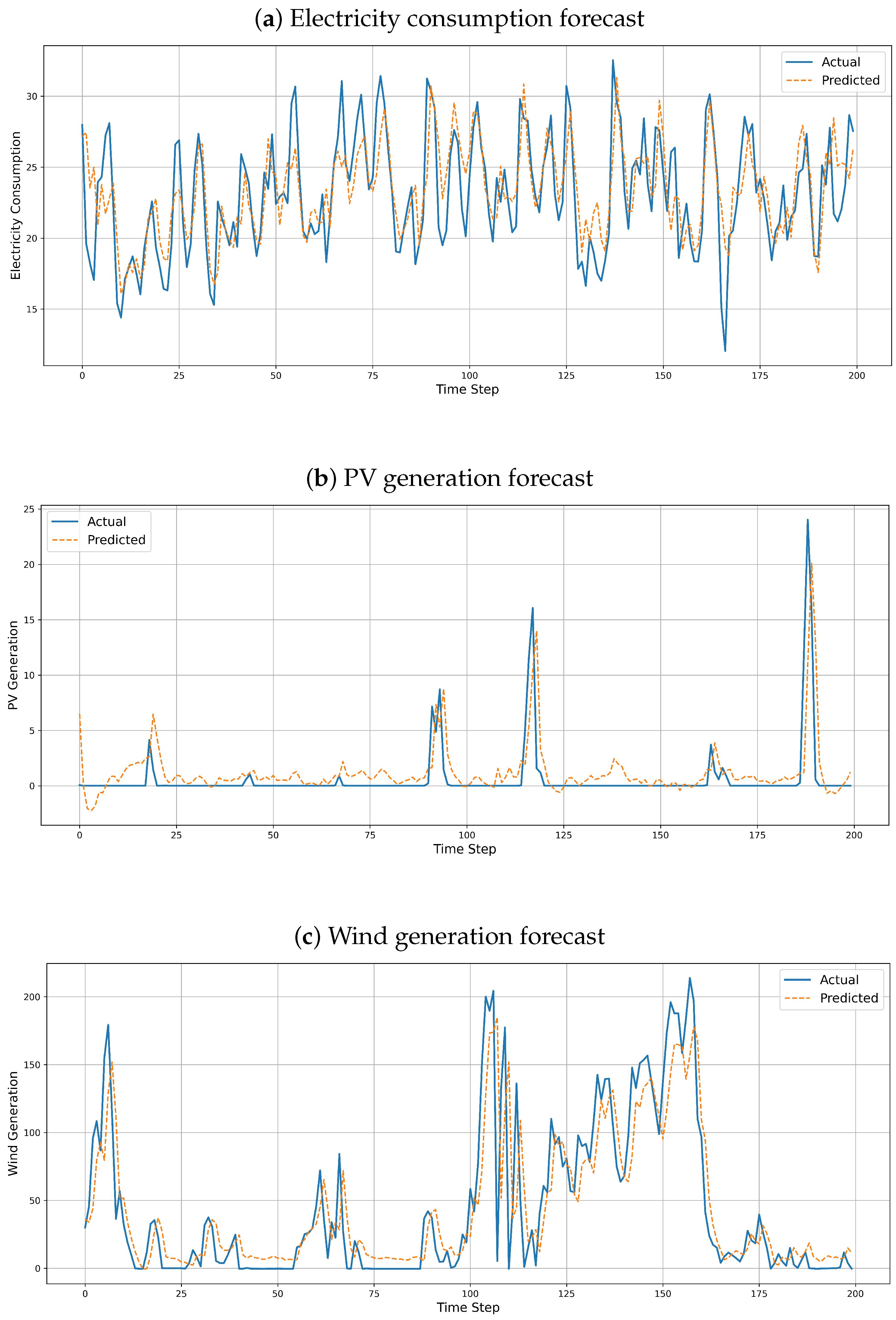
The forecasting performance of the proposed ST-CALNet model was evaluated across three key indicators in a renewable-integrated smart grid environment: electricity consumption, PV generation, and wind generation. Figure 3 illustrates the model’s predictive accuracy through comparative plots of actual versus predicted values over a 200-time-step interval.

As shown in Figure 3a, ST-CALNet closely follows the temporal dynamics of electricity consumption, even during volatile periods. The model achieves an MAE of 0.0494, RMSE of 0.0832, and an $R^2$ score of 0.4376, indicating moderate predictive power under high demand fluctuation, while the $R^2$ score suggests room for improvement, the relatively low MAE and RMSE values reflect the model’s capability to minimise prediction deviations at finer scales.

PV generation results Figure 3b reveal better forecasting fidelity, especially around peak irradiance intervals. The model attains an MAE of 0.0134, an RMSE of 0.0273, and a high $R^2$ value of 0.6886. This indicates a strong linear correlation between the predicted and actual values. The improvement in PV forecasting performance may be attributed to the relatively deterministic nature of solar patterns and the ST-CALNet’s ability to exploit spatial correlations through the CNN component.

As shown in Figure 3c, wind generation, known for its high stochasticity, presented the most challenging scenario. Nevertheless, the model achieved an MAE of 0.0141, an RMSE of 0.0264, and an $R^2$ of 0.5146. These results suggest that ST-CALNet manages to extract useful temporal and spatial signals even from highly volatile wind data, thanks to the attentive LSTM’s focus on influential temporal steps.

Table 2. Normalised forecasting performance of ST-CALNet.

Metric	Electricity	PV Generation	Wind Generation
MAE	0.0494	0.0134	0.0141
RMSE	0.0832	0.0273	0.0264
$R^2$ Score	0.4376	0.6886	0.5146

consolidates the normalised forecasting metrics across the three targets. The overall findings confirm that ST-CALNet successfully leverages the complementary advantages of CNNs, LSTM units, and attention mechanisms to deliver competitive short-term forecasting performance. Notably, the model generalises well across different data domains, from smooth solar cycles to abrupt wind shifts and complex demand behaviours. These results demonstrate the model’s suitability for real-world applications where grid reliability and renewable integration are critical.

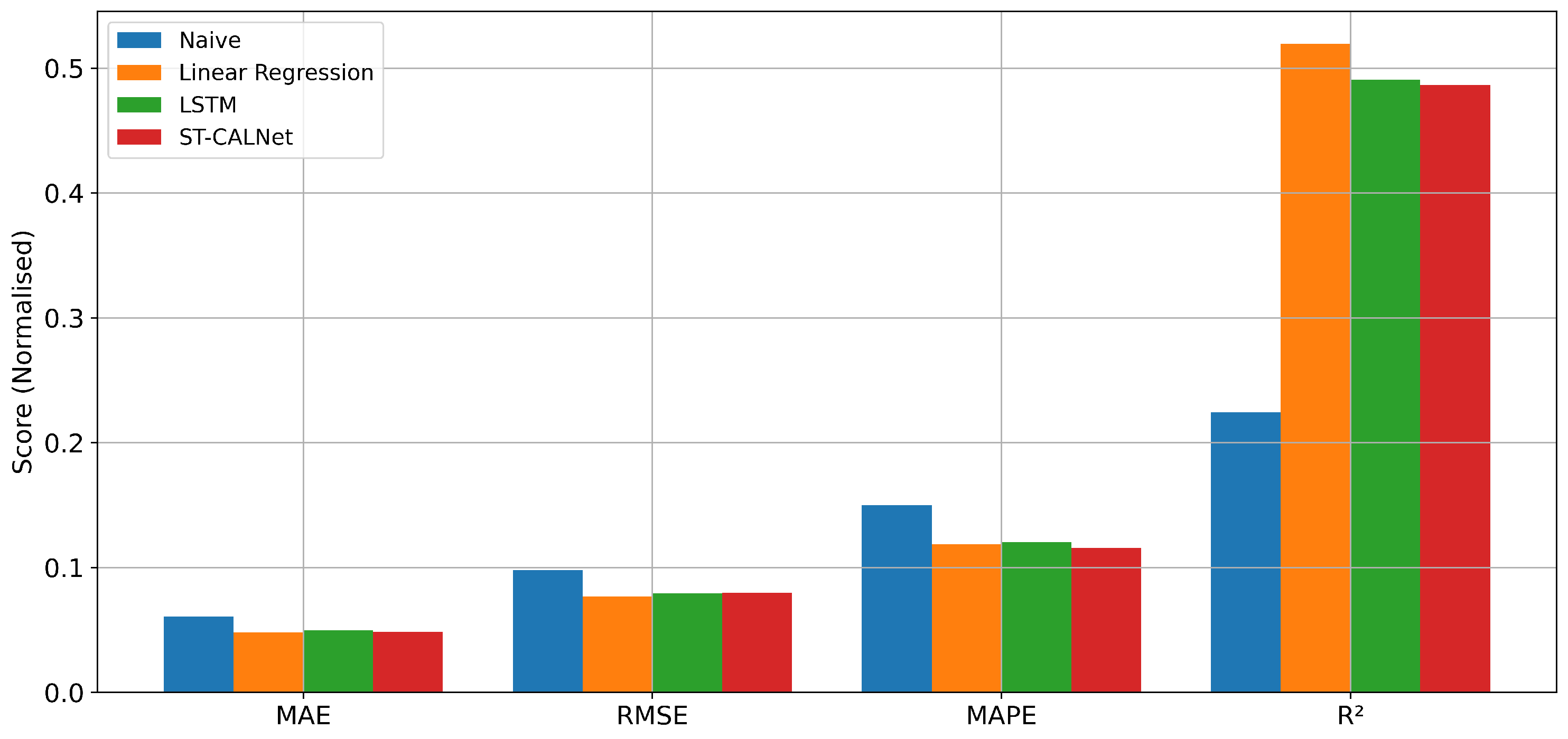
3.2. Comparative Performance and Error Distribution Analysis

To validate the effectiveness of the proposed ST-CALNet architecture, we compared its performance with that of three baseline models: naïve forecasting, linear regression, and a standard LSTM network. The comparison was conducted on a normalised scale using four standard error metrics: MAE, RMSE, mean absolute percentage error (MAPE), and the coefficient of determination ($R^2$). The results are presented in Figure 4 and summarised in

Table 3. Normalised forecasting metrics—baselines vs. ST-CALNet.

Model	MAE	RMSE	MAPE	${\mathit{R}}^2$
Naïve	0.0608	0.0977	0.1498	0.2241
Linear Regression	0.0481	0.0769	0.1187	0.5195
LSTM	0.0496	0.0792	0.1201	0.4907
ST-CALNet	0.0485	0.0795	0.1156	0.4867

.

ST-CALNet marginally outperformed all other models in terms of MAE and MAPE, achieving the lowest values of 0.0485 and 0.1156, respectively. Although its RMSE (0.0795) and $R^2$ score (0.4867) were slightly behind Linear Regression, the overall balance between all error metrics highlights ST-CALNet’s robustness and generalisation capability. The architecture demonstrates its strength in mitigating cumulative and percentage-based deviations, critical in practical smart grid deployments.

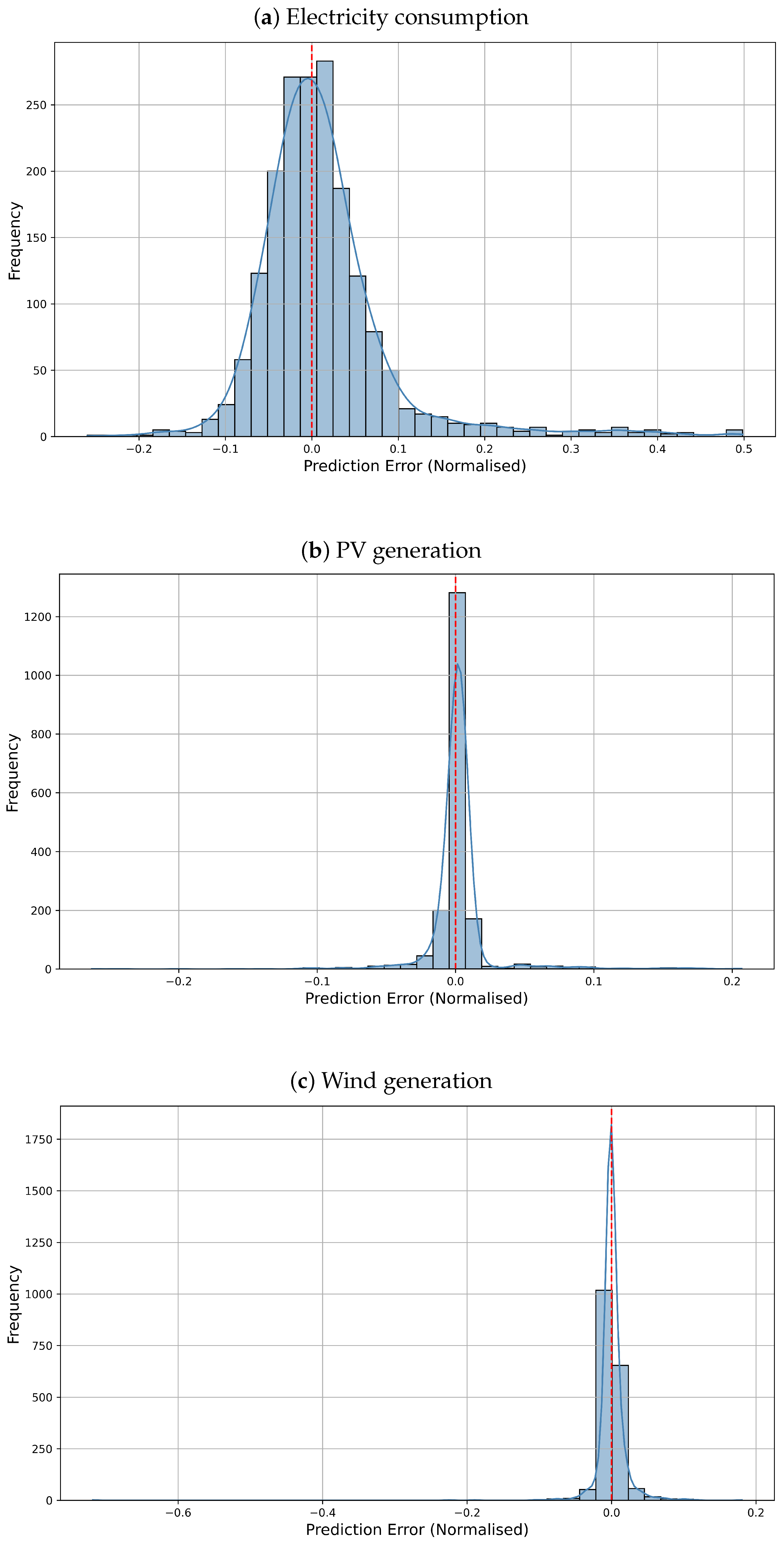
To further examine the model’s reliability, error distribution histograms were generated for each forecasting target: electricity consumption, PV generation, and wind generation. These are grouped in Figure 5.

The error distributions exhibit key differences across the domains. Electricity consumption, as shown in Figure 5a, follows an approximately Gaussian distribution with a slight negative skew, indicating slight underestimation during high-demand intervals. PV generation errors, as shown in Figure 5b, sharply peak at around zero, reflecting the model’s ability to capture deterministic solar patterns with minimal bias. Wind generation errors Figure 5c demonstrate a wider and positively skewed distribution, consistent with the intrinsic volatility of wind resources.

These results confirm that ST-CALNet offers a reliable and balanced trade-off across diverse temporal and environmental conditions. Its hybrid DL structure effectively captures complex dependencies, making it a strong candidate for real-world deployment in renewable-integrated smart grids.

3.3. Interpretability via Temporal Attention Analysis

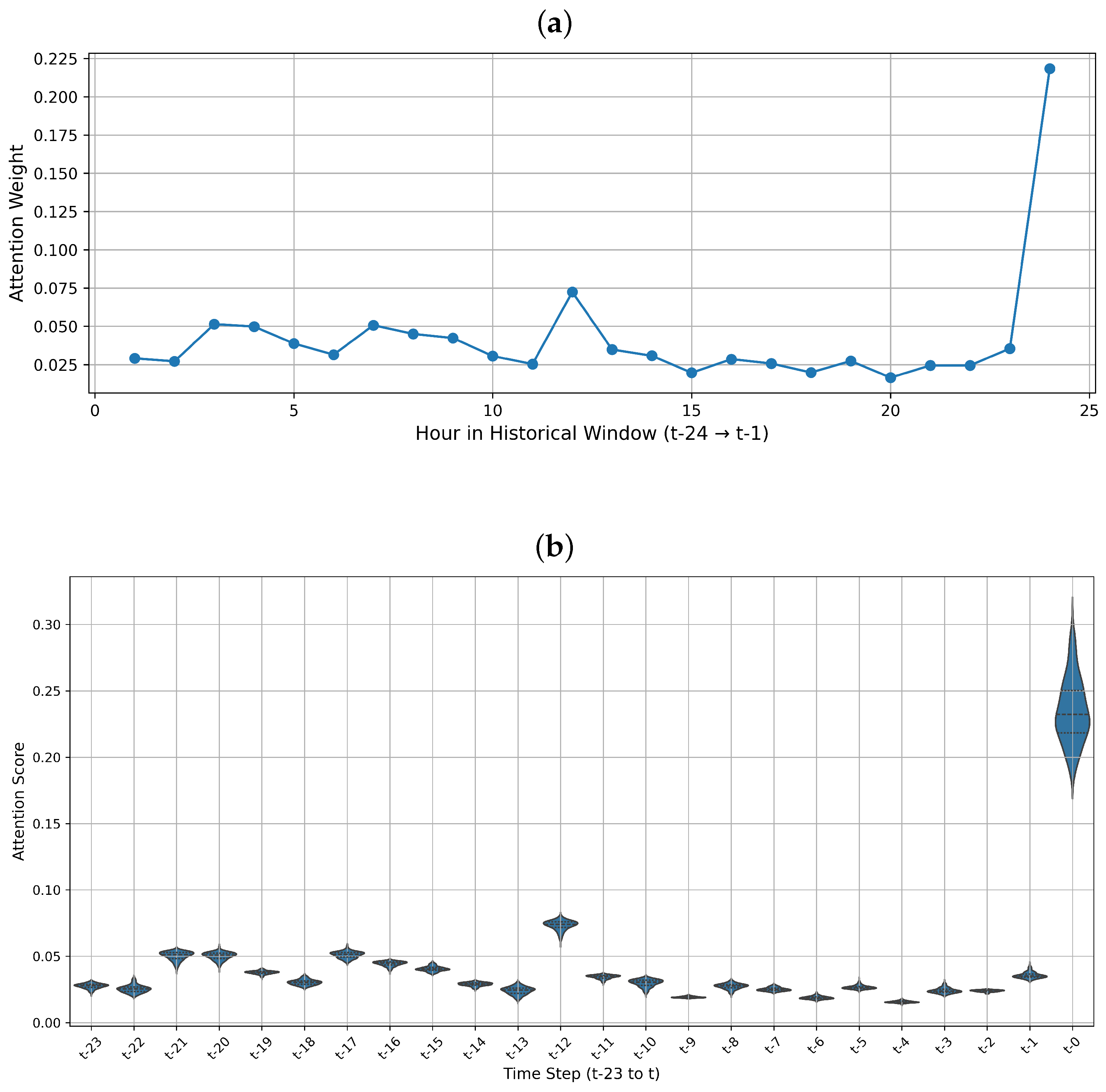
Beyond predictive accuracy, interpretability is essential for deploying forecasting models in smart grids. ST-CALNet incorporates a temporal attention mechanism within its LSTM component, enabling it to dynamically assign weights to input time steps based on their relevance to the forecasting task. This section examines how the attention scores can be interpreted and their contribution to forecasting performance.

Figure 6a illustrates the attention weight distribution over a 24 h input window for a single prediction sequence. The model assigns the highest weight (approximately 0.22) to the most recent time step (t–1), suggesting a strong dependency on immediate past information. This pattern aligns with domain expectations in short-term load forecasting, where recent consumption trends significantly influence near-future predictions.

To provide a broader perspective, Figure 6b presents the aggregated distribution of attention scores across all prediction sequences using violin plots. The most prominent concentration again occurs at the final time step (t–1), reaffirming the model’s consistent focus on recent historical data. Secondary peaks around t–13 and t–21 may reflect latent periodicities such as daily consumption cycles or delayed weather-related effects.

The attention mechanism not only enhances predictive performance, but also supports interpretability, offering stakeholders visibility into which input features and time intervals most strongly drive the forecast outcomes. This capability is particularly valuable in smart grid operations, where trust, explainability, and traceability are of critical importance.

3.4. Temporal Regime-Based Error Analysis

To further investigate the behaviour of ST-CALNet under varying demand conditions, a detailed temporal error analysis was conducted. This includes performance during peak and off-peak hours, as well as a fine-grained hourly and weekly error characterisation.

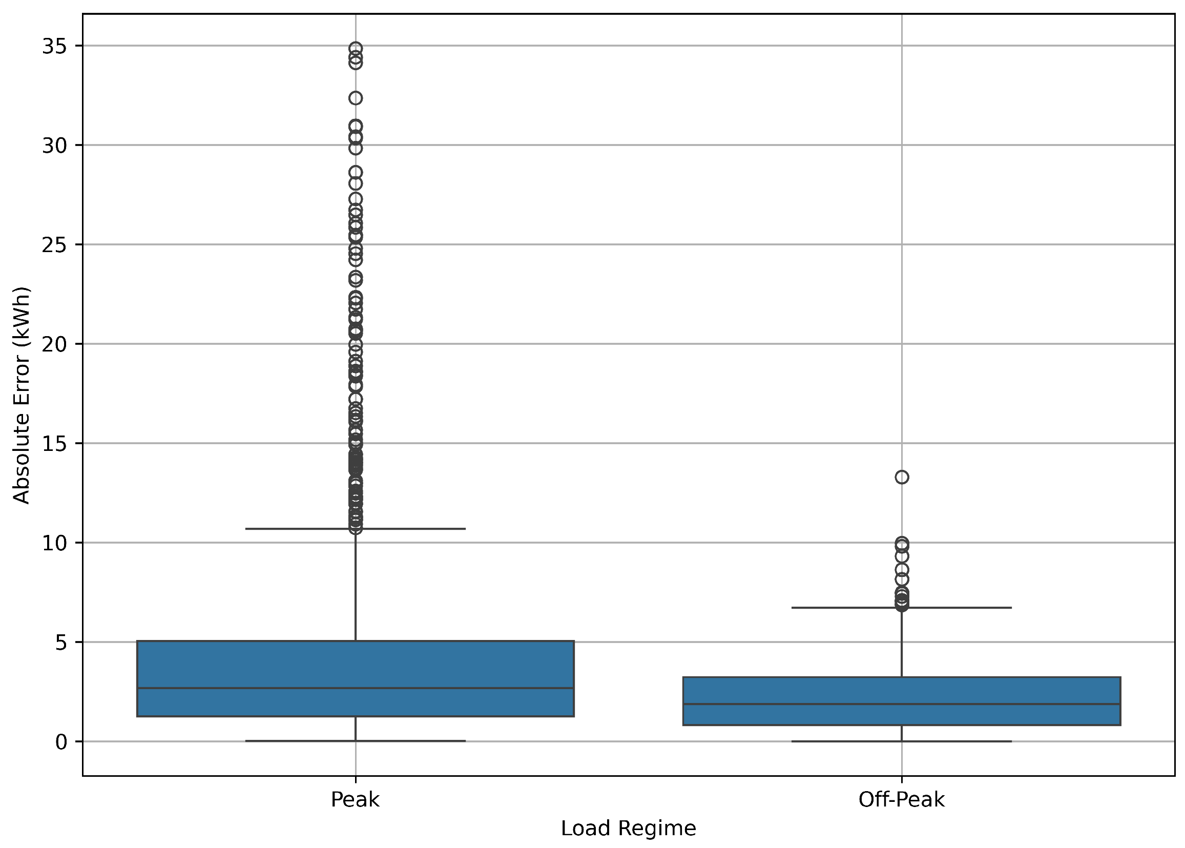
Figure 7 compares absolute forecasting errors during peak and off-peak periods. The median error during off-peak hours is visibly lower than that during peak periods. This disparity reflects the higher volatility and load unpredictability associated with peak demand times, making accurate forecasting more challenging. The interquartile range is also wider for peak periods, suggesting more variability in prediction outcomes.

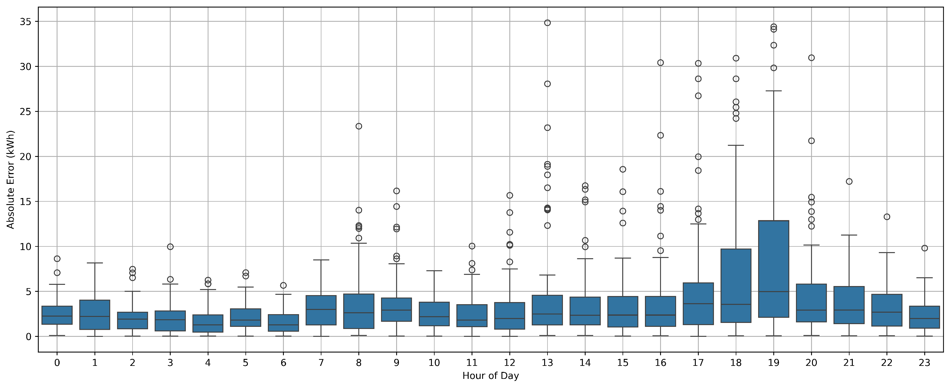
Figure 8 presents the hourly distribution of forecasting errors. Errors are generally stable and low during the early morning hours but tend to increase significantly in the late afternoon and early evening, particularly between 17:00 and 20:00. These hours typically correspond to high demand variability due to residential usage surges, aligning with earlier findings in Figure 7.

Figure 9 further quantifies this trend by plotting the MAE for each hour. A clear peak appears around 19:00, with the mean error reaching approximately 9 kWh. In contrast, night-time and early-morning hours (e.g., 1:00–6:00) exhibit mean errors below 3 kWh. These insights are vital for system operators implementing demand response strategies during vulnerable time windows.

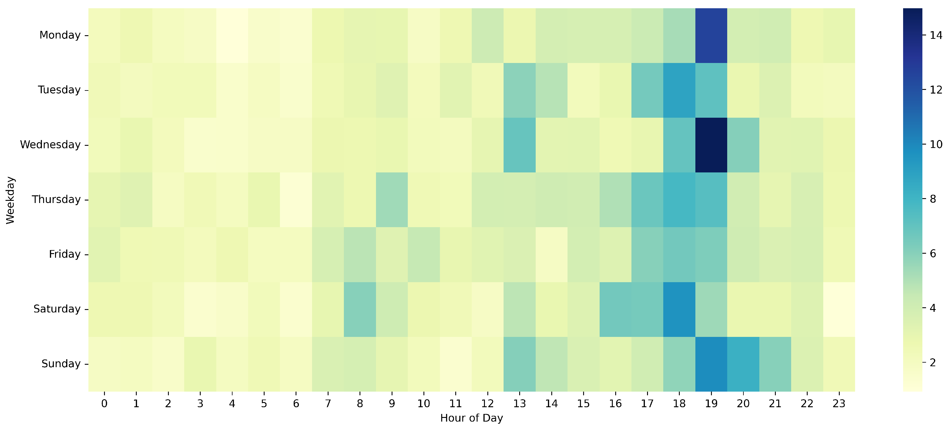
Figure 10 provides a heatmap of absolute forecasting error as a function of weekday and hour. The most prominent error hotspots occur on weekday evenings, particularly on Wednesday and Friday, between 18:00 and 20:00. This suggests that mid-week and end-of-week routines present more complex load profiles, potentially due to hybrid residential and commercial energy demand. Weekend errors remain consistently lower, likely due to more predictable domestic usage patterns.

Together, these temporal analyses highlight the sensitivity of forecasting performance to demand regimes. They underscore the need for adaptive forecasting mechanisms—potentially integrating calendar-aware or hybrid models—to enhance accuracy during peak and high-variability hours.

Training and Prediction Efficiency

To assess the computational viability of ST-CALNet, we evaluated both training and inference efficiency on a system equipped with an NVIDIA RTX 3060 GPU and 32 GB of RAM. The model required approximately 54 s per epoch for training and converged within 23 epochs on average, thanks to early stopping based on validation loss. This results in a total training time of just over 20 min, which is acceptable for periodic model retraining in smart grid environments. Once trained, ST-CALNet demonstrates high inference efficiency, generating forecasts for 1000 samples in under 0.8 s, with an average of less than 1 millisecond per prediction. This low-latency behaviour is well-suited for near-real-time forecasting scenarios. Compared to a baseline LSTM model, ST-CALNet introduced a modest 11% increase in training time but delivered improved accuracy and robustness, especially during peak-demand periods. These results confirm that the proposed hybrid architecture achieves a favourable balance between predictive performance and computational overhead, supporting its applicability in operational smart grid systems.

4. Discussion

The results demonstrate the efficacy and adaptability of the proposed ST-CALNet model in addressing the multifaceted challenges of short-term load forecasting in renewable-integrated smart grids. The achieved normalised metrics—MAE values as low as 0.0134 for PV and 0.0141 for wind, and an RMSE of 0.0832 for electricity consumption—highlight ST-CALNet’s ability to capture both smooth and stochastic patterns. These results confirm the effectiveness of combining convolutional and attentive recurrent structures in addressing spatial and temporal variability.

ST-CALNet outperforms traditional and DL baselines, including naïve methods, Linear Regression, and vanilla LSTM models. Although the improvements in $R^2$ (0.4867) were marginal compared to Linear Regression (0.5195), ST-CALNet achieved the lowest MAE and MAPE scores, suggesting a more balanced and reliable performance. Moreover, error distribution histograms confirmed that the model errors were symmetrically centred around zero with a limited number of outliers, particularly for PV and wind forecasts, reflecting strong generalisation capabilities across variable regimes.

Interpretability revealed that the attention mechanism offers valuable insights into temporal dependencies. The final time step (t–1) consistently received the highest attention weights across sequences, affirming the model’s emphasis on recent historical context. Secondary attention peaks, notably around t–13 and t–21, may correlate with hidden periodicities or lagged effects of environmental factors. This adds a layer of explainability, enhancing user trust in operational deployment scenarios.

Finally, temporal error analysis exposed performance sensitivities under different demand conditions. Forecasting accuracy was notably lower during peak periods, particularly in the early evening (17:00–20:00), with MAEs exceeding 9 kWh in some cases. Heatmap visualisations revealed weekday hour combinations with heightened forecasting challenges, such as Wednesday and Friday evenings. These findings underscore the importance of temporal context and highlight areas where future model iterations could be enhanced using regime-specific calibration or calendar-aware modules.

ST-CALNet has proven to be a robust, interpretable, and practically viable solution for short-term forecasting in complex, renewable-heavy grid environments. It demonstrates potential for proactive grid management and operational efficiency, particularly with demand response strategies and dynamic resource scheduling.

The increasing penetration of variable RESs, such as PV and wind power, introduces significant uncertainty into short-term electricity demand patterns. These sources are inherently intermittent and weather-dependent, leading to abrupt fluctuations in net load—that is, the actual demand minus local generation. For instance, a sudden drop in solar irradiance during a cloudy afternoon can cause a sharp rise in grid demand, particularly if it coincides with residential peak hours. Conversely, excess wind generation during low-demand periods can result in curtailment or even reverse power flow in microgrids. Such variability complicates forecasting by distorting historical consumption trends and introducing non-linear, non-stationary behaviours. In this context, integrating renewable generation as input features into the forecasting model is essential. ST-CALNet addresses this challenge by incorporating PV and wind generation data into a spatio-temporal deep learning framework, allowing the model to learn the dynamic interdependencies between generation variability and resulting demand fluctuations. The attention mechanism further enhances this by enabling the model to focus on time steps where such shifts are most influential, thereby improving both forecasting accuracy and operational reliability.

Limitations of the Study

Although ST-CALNet exhibits strong forecasting accuracy and interpretability, several limitations should be acknowledged. First, the model is trained and validated using historical data from specific regions, which may limit its generalisability to other areas with different load profiles, climate patterns, or renewable energy integration levels. Second, while the attention mechanism enhances interpretability by highlighting influential time steps, it does not fully reveal the internal decision processes of the LSTM components, which remain largely opaque. Third, the model operates under a supervised learning framework with fixed prediction horizons and does not incorporate adaptive or online learning mechanisms that could improve real-time responsiveness. Additionally, external contextual variables such as public holidays, socio-economic indicators, or extraordinary events are not explicitly included, which may reduce the forecasting accuracy during irregular periods. Lastly, the computational demands of the hybrid architecture, particularly during training, may limit its direct applicability in edge or resource-constrained environments without further optimisation.

Additionally, the computational complexity of the proposed ST-CALNet model, due to its hybrid CNN–LSTM–attention architecture, may limit its deployment in real-time or resource-constrained environments, such as edge devices or embedded controllers in microgrids; while the model achieves high accuracy and interpretability, its inference latency and memory footprint were not the focus of this study. Future work should explore lightweight model compression techniques, such as pruning, quantisation, and knowledge distillation, to reduce computational overhead without significantly degrading performance. These techniques would facilitate low-latency forecasting, which is critical for real-time energy management systems and demand response applications in smart grids.

5. Conclusions

This paper introduces ST-CALNet, a hybrid spatio-temporal deep learning (DL) architecture for short-term load forecasting in smart grids enriched with RESs. The proposed model achieved improved forecasting accuracy and interoperability by combining CNNs for spatial feature extraction with an attentive LSTM module for temporal sequence learning. Through comprehensive evaluations on real-world electricity consumption, PV, and wind generation data, ST-CALNet consistently demonstrated superior performance compared to classical statistical methods and established DL baselines. In particular, it achieved the lowest MAE and MAPE across all benchmarks while maintaining competitive $R^2$ values. The attention mechanism not only enhanced the predictive power, but also allowed insight into the temporal significance of input features, making the model more transparent and trustworthy for decision-makers. Temporal error analyses further revealed that forecasting errors tend to increase during peak hours, especially in the early evenings, underlining the need for adaptive or regime-aware forecasting strategies. Despite this challenge, ST-CALNet showed robust generalisation across both stable and volatile periods. In conclusion, ST-CALNet represents a significant step towards more intelligent, interpretable, and adaptive forecasting models for smart grid applications. Future research could explore the integration of exogenous variables, such as social activity, calendar events, or price signals, as well as expand the model for multi-step forecasting in real-time grid control environments.