An Improved CNN-Based Algorithm for Quantitative Prediction of Impact Damage Depth in Civil Aircraft Composites via Multi-Domain Terahertz Spectroscopy

Abstract

To address the issue of low accuracy and stability in traditional Convolutional Neural Networks (CNN)-based defect depth prediction for civil aircraft composites, we propose an improved Feature Enhancement Network (FEN)-CNN-Bidirectional Long Short-Term Memory (BiLSTM) impact damage depth prediction method. By integrating terahertz (THz) time-domain, frequency-domain, and absorbance spectroscopy with Confocal Laser Scanning Microscopy (CLSM) depth measurements, the correlation between THz spectral features and impact damage defect depth is systematically elucidated, thereby constructing a “THz features-depth” dataset. Furthermore, by leveraging the FEN model’s feature enhancement and denoising capabilities, along with the BiLSTM model’s bidirectional sequence modeling capability, the underlying relationship between terahertz spectral features and defect depth is deeply learned. This approach improves the stability and accuracy of spectral feature extraction by the CNN model under complex conditions. Ablation experiments revealed the improved model, compared to traditional CNN, reduced Mean Absolute Error (MAE), Mean Absolute Percentage Error (MAPE), Mean Squared Error (MSE), and Root Mean Squared Error (RMSE) by 43.08%, 44.4%, 57.18%, and 34.56%, respectively. Additionally, it decreased the Relative Standard Deviation (RSD) by 32.14%, and increased the Coefficient of Determination (R²) by 6.8%. Comparative experiments demonstrated the proposed model achieved an MSE of 0.0075 and an R² of 0.9539, outperforming other models. This study provides a novel method for precise low-velocity impact damage assessment in carbon fiber reinforced composites, enhancing safety evaluation for civil aircraft composite structures and contributing to aviation safety.

1. Introduction

Carbon Fiber Reinforced Plastics (CFRP) exhibit superior characteristics over other materials, including high-temperature resistance, corrosion resistance, light weight properties, and exceptional strength, which have facilitated their extensive application in the aerospace, automotive, and medical fields [1,2,3]. Notably, in the Boeing 787 and Airbus A350XWB, the proportion of CFRP utilized in structural components exceeds 50% [4,5]. However, during service, CFRP inevitably develops damage defects due to external environment factors. Among these, impact-induced damage defects caused by bird strikes, hailstones, or other external forces not only affect surface integrity but may also induce internal structural degradation, thereby affecting the performance and safety of civil aircraft structures. This type of damage has emerged as a critical factor influencing the safe operation of civil aircraft [6,7,8]. Therefore, the timely identification and remediation of these impact-induced defects are particularly crucial for ensuring flight safety.

Terahertz (THz) technology, as an emerging nondestructive testing method, exhibits several advantages over other methods, including excellent penetration capability, non-ionizing properties, and high safety for various non-metallic and non-polar materials [9,10,11]. Consequently, it has been widely applied in diverse fields such as precise ranging, coating thickness measurement, and surface morphology characterization [12,13,14]. Particularly within the field of nondestructive testing, numerous THz analysis and processing methods have been proposed by scholars. For instance, Zhong et al. reported that THz spectral characteristics exhibit a linear relationship with defect parameters in CFRP materials [15]. However, this method is constrained by its reliance on simple linear models, which inherently assume an idealized and resolvable direct correspondence between THz signals and defect characteristics. This assumption often proves insufficient and fails to address complex signal variations caused by deformation in defect surface morphology, particularly when faced with the complex, irregular defect morphologies commonly found in real-world components. In such cases, these linear assumptions tend to break down, leading to a significant decrease in prediction accuracy. Li et al. developed an approach involving features extraction from THz signals followed by multi-feature fusion, enabling accurate assessment of material porosity and thereby demonstrating the feasibility of multi-feature fusion [16]. Wang et al. proposed a technique combining terahertz time-domain signals with a one-dimensional convolutional neural network (1D-CNN), achieving effective prediction and classification of internal defect depth in composite materials [17]. This method achieved a highest recall rate of 0.97 and a macro-F1 exceeding 0.91. Zhang et al. further advanced the field by employing a hybrid CNN-RSN-SVM model for thickness classification of CFRP defects, achieving an accuracy of 98.91% [18]. However, these models still demonstrate significant limitations, as they are only capable of achieving discrete classification tasks and thus struggle to meet high-precision quantitative requirements. This challenge in transitioning from classification to precise quantification suggests that the models may struggle to capture the subtle signal patterns inherently associated with continuous depth variations. This limitation primarily arises from the restricted number of input features within the model, which prevents the effective capture of the complex interrelationships between features and depth. This issue may signify a bottleneck in current feature engineering, where the selected features might inadequately represent the geometric and physical attributes of defects, or, alternatively, reflect that the model architectures themselves are ill-equipped to handle the intricate non-linear mappings in high-dimensional feature spaces. Consequently, establishing a precise correspondence between THz signal characteristics and damage depth becomes increasingly challenging. In addition, the complex and variable surface morphology of impact-induced damage in CFRP can lead to significant variations in reflected terahertz signals [19,20]. These variations not only encompass defect-related information but also introduce substantial noise and interference unrelated to the actual defects. Unfortunately, existing methods often lack robust mechanisms for effectively differentiating and suppressing these surface scattering effects. Furthermore, variations in surface geometric structure can induce scattering and diffraction of THz waves, thereby increasing the complexity of the signals [21,22,23]. On the other hand, conventional THz signal data processing methods face difficulties in simultaneously addressing local feature extraction and global information integration, thus complicating the establishment of a precise quantitative relationship between THz spectral features and damage depth.

In summary, the existing research predominantly exhibits three major limitations. First, current methodologies excessively depend on single-domain THz spectral features [24], which impedes the effective utilization of multi-domain features and consequently hinders the comprehensive intricate characterization of materials. Second, existing algorithms have not yet to establish a clear one-to-one mapping between spectral features and depth values, particularity for arbitrary depths. Moreover, previous studies have predominantly focused on classification tasks rather than delivering precise quantitative analysis. Third, current models reveal insufficient capacity for enhancing and reconstructing THz characteristic signals as well as capturing long-term dependencies. This limitation suggests that models might encounter difficulties in extracting critical depth-sensitive information from noisy or attenuated raw signals and may be unable to leverage the contextual relationships within the feature sequences of the signal—relationships that are essential for ensuring stable model interpretation. Collectively, these limitations result in inadequate prediction accuracy in assessing impact-induced damage depth within the existing research.

To address the aforementioned challenges, we propose an improved FEN-CNN-BiLSTM model for accurately predicting the depth of impact-induced damage defects in CFRP. Multi-domain feature representations are constructed by integrating various types of THz spectral features. The morphology and depth of the defects are quantitatively characterized using Confocal Laser Scanning Microscopy (CLSM), with the depth serving as the ground truth label for the model samples. Consequently, a comprehensive dataset containing multiple features and corresponding depth values is established. By processing feature noise through the Feature Enhancement Network (FEN) module to enhance signal quality, leveraging Convolutional Neural Network (CNN) for extracting local features, and combining it with Bidirectional Long Short-Term Memory (BiLSTM) to capture inter-feature dependencies, precise prediction of the impact damage depth is achieved. The main contributions and innovations of this study can be summarized as follows:

• By combining THz multi-domain features with the defect depth obtained via CLSM, an innovative “THz Spectral Features-Defect Depth” (TSF-DD) dataset for CFRP was systematically constructed, providing a solid foundation for the precise quantitative analysis of low-velocity impact damage depth in CFRP materials.
• We propose a novel deep learning model, FEN-CNN-BiLSTM, which represents the innovative application of this hybrid model specifically to the depth regression prediction of CFRP defects in civil aircraft. The proposed method achieves high-accuracy prediction of continuous depth values for CFRP impact damage defects, providing new perspectives and methodologies for non-destructive testing within the field of civil aviation.
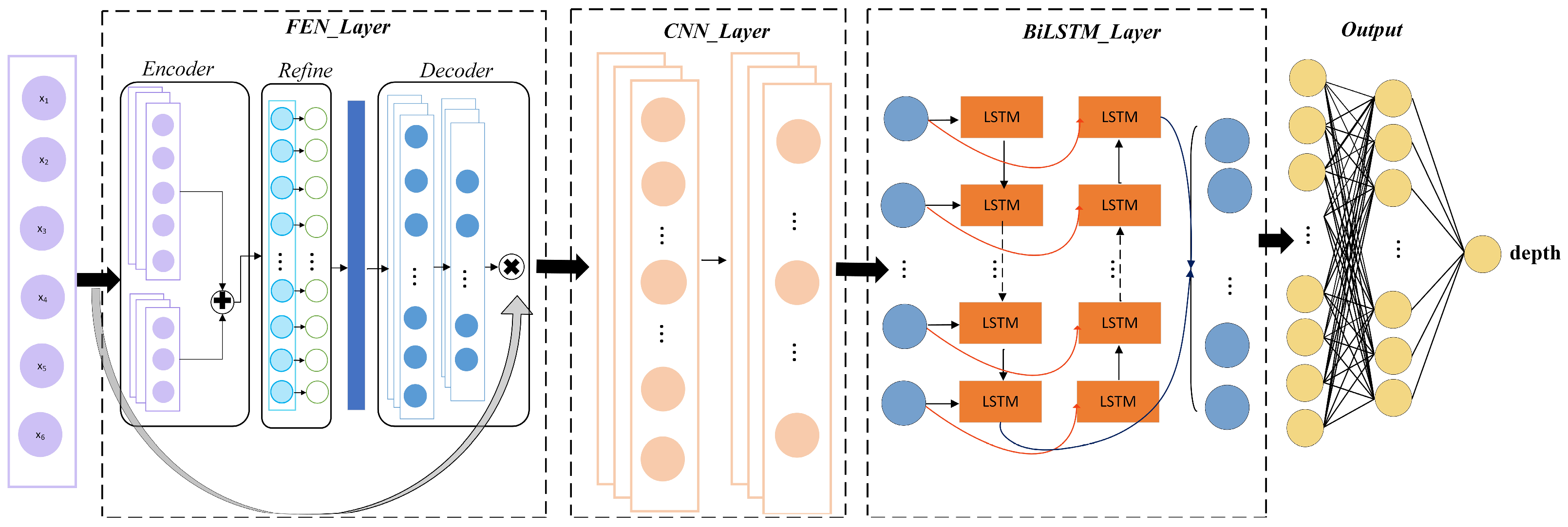
• The improved FEN-CNN-BiLSTM model is specifically designed to address THz spectral characteristics and incorporates an innovative FEN module. This module achieves feature recombination and purification through a simplified encoder-decoder-like architecture, effectively mitigating information loss. Additionally, the BiLSTM bidirectional modeling mechanism comprehensively investigates the inter-feature correlations, enhancing the model’s capability to understand complex features. Consequently, this model significantly enhances the accuracy and stability of predictions regarding the depth of impact damage defect.

2. Theory and Methods

THz spectroscopy technology enables the extraction of optical parameters and structural information from impact-damaged materials by analyzing their response to THz pulses. Reflection-mode signals can be analyzed in the time-domain, frequency-domain, and absorbance spectrum to characterize the damage characteristics of CFRP materials.

2.1. Time-Domain Signal

The Time of Flight (TOF) of the THz pulse to the material surface can serve as an indicator for detecting variations in the material surface topography [25]. The distance d from the instrument probe to the material surface is estimated using the following equation:

$$d={\displaystyle \frac{ct}{2n}} ,$$

(1)

where c is the propagation velocity of electromagnetic waves, t represents the round-trip time of the pulse traveling from the probe to the sample surface, and n can be approximated as 1 in air. The variation in TOF directly reflects the surface depression depth caused by impact damage. The peak intensity of the reflected signal corresponds to the degree of signal attenuation.

2.2. Frequency-Domain Signal

To investigate the reflection and transmission characteristics of THz waves on the material surface and within its interior, the time-domain signal was subjected to Fourier transform [26] to obtain frequency-domain amplitude and phase information as follows:

$$\tilde{E}\left(\omega \right)=F\left\{E\left(t\right)\right\} ,$$

(2)

where ω is the angular frequency and F denotes the Fourier transform. When the material sustains damage from impact, in addition to surface pit formation, complex internal damage such as matrix cracking and fiber breakage may also occur. These damages modify the original reflection characteristics by increasing scattering and absorption losses, which in turn affect the propagation of THz waves. These variations cause changes in the frequency-domain amplitude and phase of the reflected signal. Therefore, the analysis of frequency-domain signals provides a basis for evaluating the extent of impact-induced damage.

2.3. Absorbance Signal

Absorbance is typically utilized to quantify the absorption capacity of a material with respect to THz waves. The absorbance, denoted as A, can be mathematically expressed by the following equation [27]:

$$A=-\lg \left({\displaystyle \frac{I}{ I_0}}\right) ,$$

(3)

where I₀ is the incident power, I is the transmitted power, and d1 is the sample thickness. Impact-damaged regions modify the propagation path of THz waves, leading to alterations to the absorbance spectral characteristics. Quantitative analysis of these patterns of absorbance variation allows for the effective analysis of the degree of defect damage severity.

3. Experiment and Data Analysis

3.1. Sample Preparation

The experimental samples were composed of impact-damaged CFRP specimens with dimensions of 50 mm × 50 mm × 5 mm. The presence of impact damage was identified using the reflection module of the THz scanner. The acquired data included THz time-domain, frequency-domain, absorbance spectra, and corresponding images of the samples of the specimens. During the experiment, continuous nitrogen purging was performed to eliminate the interference caused by water vapor on the measurement results. A CLSM was utilized to scan the sample surface for obtaining precise depth information. The detailed scanning parameters are listed in

Table 1. Experimental instrument parameters.

Category	Parameter	Value
THz Scanning Parameters	Instrument Model	CCT-1800
	Spectral Range	0.06 THz–4 THz
	Dynamic Range	80 dB
	Minimum Step Size	0.08 mm
	Positioning Accuracy	2 μm
CLSM Scanning Parameters	Instrument Model	OLS4100
	Light Source	405 nm semiconductor laser
	Z-axis Travel Range	10 mm
	Accuracy error	<0.5 μm
	Positioning Resolution	10 nm
Scanning Environment	Temperature/Humidity	23 °C/45%

.

3.2. THz Imaging Results and Multi-Feature Depth Analysis

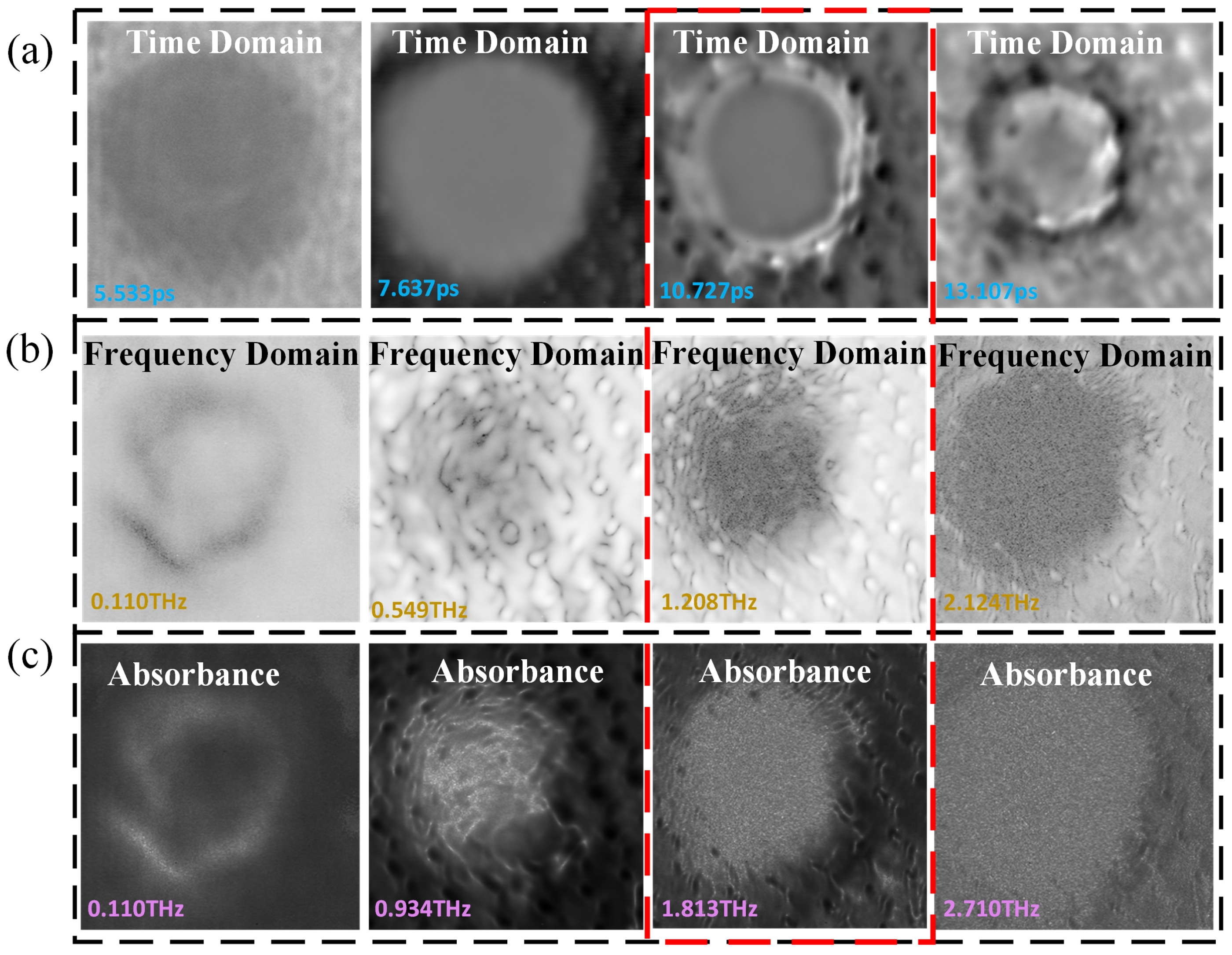
3.2.1. Imaging Analysis

The impact-damaged regions of the CFRP were analyzed using THz time-domain, frequency-domain, and absorbance imaging techniques. The experimental results obtained under various imaging parameters are presented in Figure 1.

A comparison of the imaging effects under various parameters is presented in Figure 1. The results revealed that the boundaries of the damaged region were sharply defined and exhibited high contrast when the time-domain pulse duration was set to 10.533 ps, the frequency-domain frequency was configured to 1.208 THz, and the absorbance imaging frequency was denoted as 1.813 THz. These conditions indicate that the reflection, transmission, and absorption characteristics of THz waves effectively highlight the features of the damaged region. In subsequent sections, a detailed analysis of the specific characteristics within various locations of the damaged region and their correlation with depth will be investigated through a combined analysis of CLSM data and spectral analysis.

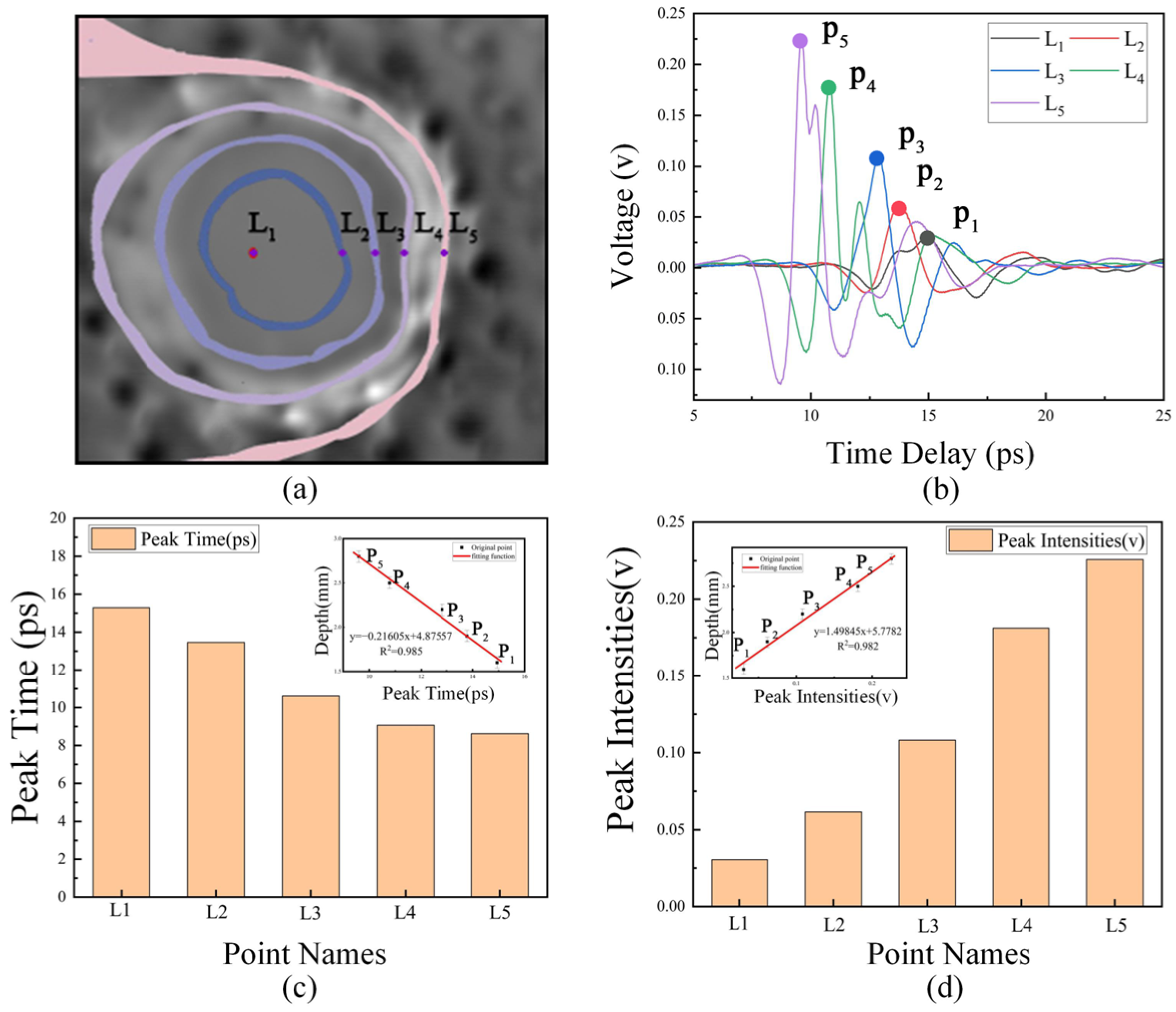
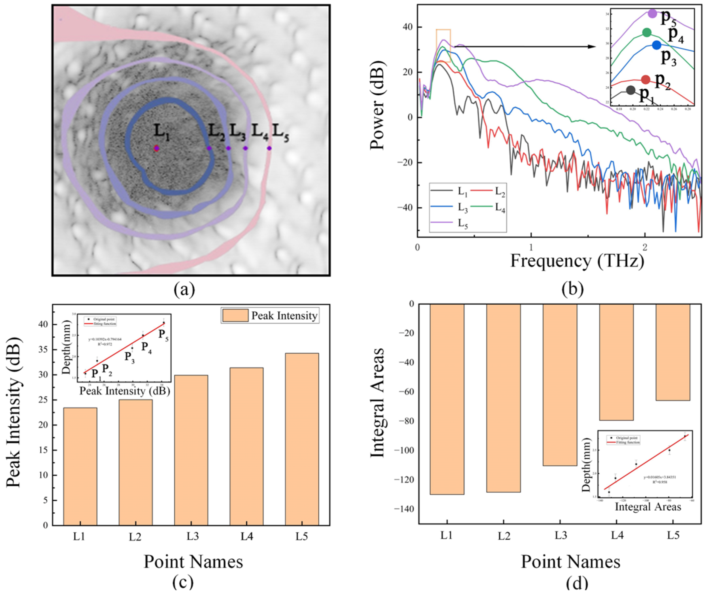
3.2.2. Depth-Based Spectral Point Selection

The three-dimensional topography and precise depth data of the damaged region of the sample were acquired using CLSM. The region was segmented into five levels at equal depth intervals, extending radially from the damage center to the periphery, with distinct color codes assigned for clarity, as depicted in Figure 2. Figure 2a presents a photograph of the CLSM scanning area on the sample, clearly revealing the depressed damage in the central region. Figure 2b illustrates a top-view point cloud of the damaged region, divided into five zones at equal depth intervals from shallow to deep, marked by central points colored pink, light purple, purple, blue, and red, respectively. Figure 2c shows a front-side view of the damaged region, clearly displaying the contour of the depression. Figure 2d provides an oblique top-view, further illustrating the depth variation within the damaged region. These visualizations provide accurate spatial position references for subsequent THz spectral analysis.

3.2.3. THz Multi-Feature Depth Analysis

Under optimal imaging parameters, five representative positions ranging from L₁ to L₅ were selected according to contour lines for spectral analysis. Subsequently, six characteristic parameters were extracted to evaluate the correlation between THz spectral characteristics and the measured defect depths.

Under the parameter condition of 10.533 ps, THz time-domain imaging was conducted on the sample. In the imaging map shown in Figure 3a, five measurement points (L₁ to L₅) were selected according to the depth contours of the defect sample. Figure 3b shows the THz time-domain spectra corresponding to these points, where P₁ to P₅ indicate the positions of the peaks in the THz spectra for each respective point. Figure 3c illustrates the TOF characteristics of the spectra for each point, while Figure 3d displays the peak intensity of the time-domain spectra for each point.

Figure 3c,d exhibit a strong linear correlation between the impact damage depth and the characteristics of the THz time-domain signal. When THz waves propagate through composite material, impact-induced damage defects cause scattering, absorption, or reflection of the THz wave energy. For deeper defects, the increased propagation path leads to more significant signal attenuation, thereby causing an extended TOF and reduced peak intensity. Conversely, for shallower defects, the shorter reflection path result in less signal loss, resulting in a decreased TOF and enhanced signal intensity. The coefficient of determination (R²) further demonstrates that the strong linear relationship between defect depth and both the THz spectral TOF (R² = 0.9856) and THz peak intensity (R² = 0.9824).

Under the condition of 1.208 THz, THz frequency-domain imaging was conducted on the sample. In the frequency-domain imaging map, as shown in Figure 4a, five measurement points (L₁ to L₅) were selected based on equidistant sample depths. Figure 4b shows the THz frequency-domain spectra corresponding to these measurement points, where P₁ to P₅ indicate the positions where the peaks in the THz frequency-domain spectra are observed. Figure 4c illustrates the peak intensity of the frequency-domain spectra for each point, while Figure 4d reflects the integral area of the spectral signal for the measurement points.

The fitting curves presented in Figure 4c,d indicate a strong linear correlation between the impact damage depth and the characteristics of the THz frequency-domain signal. As the defect depth increases, the THz wave propagates over a greater distance, during which a portion of its energy is absorbed or scattered. Consequently, the returned signal becomes weaker, leading to reduced peak intensity in the frequency-domain and a smaller integral area. Conversely, shallower defects exert less impact on the THz wave, leading to stronger reflected signals, higher peak intensities, and larger integral area. Furthermore, the coefficient of determination (R²) confirms a high degree of linear correlation between the defect depth and both the THz frequency-domain signal peak intensity (R² = 0.9723) and the frequency-domain spectral integral area (R² = 0.9581).

Under the condition of 1.813 THz, THz absorbance imaging was conducted on the sample. Figure 5a presents the absorbance imaging map, where five measurement points (L₁ to L₅) were selected based on equidistant sample depths. Figure 5b shows the THz absorbance spectra corresponding to these points, with P₁ to P₅ indicating the peak positions in the spectra. As shown in Figure 5c, the absorbance peak intensity decreases gradually as the defect depth diminishes. Figure 5d shows the selected characteristic values of the absorbance baseline, which represents the average absorption intensity level of the sample for THz waves.

The fitting curves presented in Figure 5c,d indicate a distinct relationship between the impact damage depth and the characteristics of the THz absorbance signal. Specifically, when defects are relatively deep, the THz waves propagating within the material experience significant absorption or scattering, resulting in higher absorbance peak intensities and elevated absorbance baseline values. Conversely, shallower defects exert a reduced effect on the THz waves, resulting in weaker absorption or scattering effects, which manifest as lower absorbance peak intensities and reduced baseline values. Furthermore, the coefficient of determination (R²) confirms a strong linear correlation between the defect depth and the THz absorbance signal peak intensity (R² = 0.9887), and a quadratic correlation between the defect depth and the THz absorbance spectral baseline (R² = 0.9586).

In summary, as the defect depth decreases, the TOF of the THz time-domain signal decreases, the peak intensity increases, and both the frequency-domain peak intensity and the signal integral area exhibit an upward trend. Additionally, the absorbance peak and baseline values decrease.

Table 2. Pearson coefficients for each characteristic value.

Feature Category	Features Name	Pearson Coefficient	Correlation Strength
Time-domain	Peak Time	0.993	strong positive correlation
	Peak Value	−0.991	strong negative correlation
Frequency-domain	Peak Intensities	−0.986	strong negative correlation
	Integral Areas	−0.979	strong negative correlation
Absorbance	Peak Intensity	0.994	strong positive correlation
	Baseline absorbance	0.942	strong positive correlation

below further demonstrates the correlation between the characteristic values and depth. Notably, a Pearson coefficient with an absolute value closer to 1 indicates a stronger correlation.

These changes comprehensively reflect the propagation, absorption, and scattering characteristics of THz waves in defect regions at various depths from multiple perspectives. Specifically, the coefficients of determination (R²) between the selected characteristics and depth are consistently greater than 0.95, and the Pearson coefficients indicate a strong linear relationship. This demonstrates the existence of a reliable quantitative association between the THz time-domain, frequency-domain, and absorbance characteristics and the depth of damage. These findings can serve as critical indicators for the evaluation of CFRP damage depth, laying a solid foundation for the subsequent construction of datasets based on these characteristics.

4. Multi-Feature Depth Prediction Model

In this study, we propose an impact damage depth prediction model based on THz spectral multi-features. The overall procedure is illustrated in Figure 6. Initially, the impact-damaged samples are scanned using a THz imaging system, and spectral features are extracted by combining time-domain, frequency-domain, and absorbance signals. Subsequently, CLSM is employed to acquire point cloud data, which, after depth extraction, serves as the ground truth labels for the model. The THz spectral feature data and corresponding depth labels are combined into form a dataset for model training. Finally, the prepared dataset is input into the proposed model and processed sequentially through each module within the model to achieve precise prediction of impact damage depth.

4.1. Dataset Preparation

In this study, terahertz spectral and CLSM data are acquired, initially consisting of 77,137 original sampling points obtained by scanning the entire sample surface. To address the computational complexity arising from such a large dataset, a “step-sampling” strategy was implemented (steps 1–5 tested). Specifically, a step of 3 refers to selecting one sampling point for every 3 sampling points along both the horizontal and vertical coordinates of the original sampling points. This uniform sampling approach retains 1/9 of the original points, thereby significantly reducing the data volume. The optimal sampling density was determined by evaluating three key metrics: Mean Nearest Neighbor Distance (MNND), Mean Entropy (ME), and Mean Variance (MV). MNND reflects spatial density, with smaller values indicating higher point density. ME reflects information diversity, where larger values indicate richer information content. MV reflects feature coverage, with larger values indicating wider feature variation coverage. As shown in

Table 3. Comparison of evaluation metrics at different dteps.

Sampling Interval	MNND	ME	MV
1	0.548772	1.8007367	34,376.13
2	0.831841	1.8162872	34,383.62
3	1.043408	1.8572339	34,877.77
4	1.313768	1.8755792	34,795.24
5	1.594213	1.8863185	35,572.18

, a step of 3 was selected. This choice resulted in a moderate MNND value of 1.04, effectively avoiding the problems of excessive data density and high redundancy associated with steps 1 and 2, as well as the issue of over-sparsity affecting representativeness associated with steps 4 and 5. Simultaneously, its ME (1.857) was significantly higher than that of step 2, and it exhibited the highest MV value, indicating substantially enhanced information diversity and broader coverage of feature variations, thus better reflecting the characteristics of the original data.

Through this sampling method, a total of 8526 data points were systematically collected. For each data point, six key spectral features were extracted: time-domain peak time, time-domain peak value, frequency-domain peak intensity, frequency-domain integrated area, absorbance peak intensity, and absorption baseline value. Based on these six features as input variables and the depth measured by CLSM as labels, a dataset was constructed. Subsequently, this main dataset was divided into two subsets: 70% for model training and 30% for testing. This training subset underwent five-fold cross-validation, and the model exhibiting the best performance during validation was selected for subsequent testing. To evaluate the generalization capability of the model, an independent external dataset was used. This dataset consisted of 2215 terahertz spectral data points along with corresponding CLSM-measured damage depths obtained from actual impact-damaged aircraft skin components.

4.2. Model Design Overview

Preliminary experiments indicated that employing the single-feature TOF input for the entire dataset, which contained noise and material variations, yielded a validation set performance of R² = 0.83. This suboptimal outcome can primarily be attributed to the following factors: (1) Variations within the damaged area, including changes in fiber orientation and local density, significantly affected the propagation characteristics of THz waves. (2) Difference in signal-to-noise ratio (SNR) across various regions of the sample rendered the single-feature approach insufficiently informative and unstable, making it unsuitable as a reliable basis for accurate predictions. (3) The initial selection of five representative points at various depths could only demonstrate the existence of a correlation but failed to comprehensively capture all variations across the entire defect region. Conversely, the complete feature dataset captures the full spatial diversity of the composite material damage regions, thus increasing the complexity of predictive modeling. The observed performance degradation suggests that in practical applications, basic deep learning models relying on a single feature are susceptible to issues such as high sensitivity to THz signal noise, significant prediction errors, and inadequate stability.

To address these issues, it is essential to construct a multi-feature dataset. Based on this dataset, we propose a novel multi-feature input depth prediction model that combines the FEN, CNN, and BiLSTM. To mitigate the issue of THz signal noise interference, an innovative lightweight FEN module was designed to perform feature reorganization and enhancement on the input features. Subsequently, CNN was utilized to extract local features. Finally, a BiLSTM module was employed to capture the correlations among features, enhancing the model’s ability to understand complex features. A prediction model was established using six features, including time-domain TOF peak and frequency-domain peak intensity, as inputs, with pit depth serving as the output. The FEN-CNN-BiLSTM model structure is shown in Figure 7.

4.2.1. FEN Module

The FEN module draws inspiration from the AutoEncoder paradigm and is specifically designed to effectively leverage multi-feature information for THz spectral analysis. Unlike conventional AutoEncoders, which emphasize data compression through complex architectures, FEN utilizes a lightweight, symmetric encoder-refinement-decoder architecture that not only reduces computational complexity but also preserves feature integrity.

Within the FEN module, input X is processed through parallel feature extraction paths ρ5 and ρ3 with kernel sizes of 5 and 3 respectively, generating concatenated encoded features as shown in Equation (4).

$$E={\rho }_e\left(x\right)={\rho }_3\left(x\right)\oplus {\rho }_5\left(x\right)$$

(4)

An attention mechanism computes channel weights to calibrate the encoded features E, as described in Equation (5).

$$W_a=\sigma \left({\gamma }_a\times BN\left(W_a\ast AvgPool\left(E\right)+b_a\right)+{\beta }_a\right) ,$$

(5)

where ∗ denotes the 1D convolution, BN represents Batch Normalization (including learnable affine parameters γ and β), σ is the activation function, and AvgPool signifies Global Average Pooling along the sequence length dimension.

These weights are element-wise multiplied with E to produce the modulated sequence in Equation (6).

$$H_a=E\odot W_{a }$$

(6)

The modulated features then undergo an enhancement process to yield refined features, as shown in Equation (7).

$$H_r=\sigma \left({\gamma }_e\times BN\left(W_e\ast H_a+b_e\right)+{\beta }_e\right)$$

(7)

The decoder reconstructs Hr to match the input dimensionality in Equation (8), then integrates with the original input X via residual connection to produce the final output Y in Equation (9).

$$H_d=\sigma \left({\gamma }_d\times BN\left(W_d\ast H_r+b_r\right)+{\beta }_r\right) ,$$

(8)

$$Y=F_{\mathrm{rec}}+x$$

(9)

4.2.2. CNN Algorithm

The CNN algorithm achieves regression prediction through the integration of convolutional layers, feature dimensionality reduction modules, and fully connected layers [28]. Typically, it consists of the following parts: Convolutional layers employ convolutional kernels to conduct convolution operations on the input sequence, thereby extracting local features and capturing nonlinear relationships within the input data. Pooling layers are generally located subsequent to convolutional layers. In this study, traditional pooling layers are replaced by channel compression to reduce feature redundancy while preserving key information. The formula for convolution calculation is presented below.

$$x_j^{\left(l\right)}=\Phi \left(\sum _i{x}_i^{\left(l-1\right)}\ast k_{i,j}^{\left(l\right)}+b_j^{\left(l\right)}\right),$$

(10)

where $x_j^{\left(l\right)}$ represents the j-th output sequence of the l-th layer, the symbol ∗denotes the one-dimensional convolution operation, Φ(∙) is the activation function, $k_{i,j}^{\left(l\right)}$ is the component of the j-th convolutional kernel in the l-th layer corresponding to the convolution over the i-th input sequence, and $b_j^{\left(l\right)}$ is the bias term corresponding to the j-th convolutional kernel in the l-th layer.

4.2.3. BiLSTM Structure

BiLSTM is a specialized recurrent neural network structure that comprehensively captures of dependency relationships within feature sequences by leveraging bidirectional information flow and gating mechanisms [29]. This bidirectional processing capability distinguishes BiLSTM from traditional LSTM networks, which process sequences unidirectionally. While standard LSTMs consider information flow in a single direction and may fail to fully capture the interdependencies between features, resulting in incomplete feature modeling. BiLSTM overcomes this limitation by processing information from both forward and backward directions simultaneously. This approach allows BiLSTM to build a more comprehensive representation of the sequence, thereby allowing it to effectively model complex feature associations between features and generally achieve higher prediction accuracy. In the context of THz feature processing, BiLSTM models the extracted multi-spectral features as a sequence. Specifically, the forget gate determines which information to discard from the cell state of the previous time step, as shown in Equation (11). Subsequently, the input gate determines which current information should be stored, as shown in Equation (12). Based on these two operations, the cell state is updated accordingly, as illustrated in Equation (13). Finally, the output gate integrates the forward hidden state and the backward hidden state, as demonstrated in Equation (14), calculating the complex correlations between features modeled from both the forward and backward directions.

$$f_t=\sigma \left(W_f\cdot \left[h_{t-1},x_t\right]+b_f\right),$$

(11)

$$i_t=\sigma \left(W_i\cdot \left[h_{t-1},x_t\right]+b_i\right),$$

(12)

$$C_t=f_t\odot C_{t-1}+i_t\odot \mathit{tanh}\left(W_C\cdot \left[h_{t-1},x_t\right]+b_C\right),$$

(13)

$$h_{\mathrm{out}}=\left[h_{forward};h_{backward}\right],$$

(14)

where x_t represents the input feature vector at time step t; h_t−1 represents the hidden state of the previous time step; W_f, W_C, W_i are the weight matrices for each gate; b_c, b_f, b_i are the corresponding bias terms; σ is the sigmoid activation function; ⊙ denotes element-wise multiplication; h_forward and h_backward represent the outputs of the forward and backward LSTM, respectively; and the final bidirectional representation is formed through concatenation.

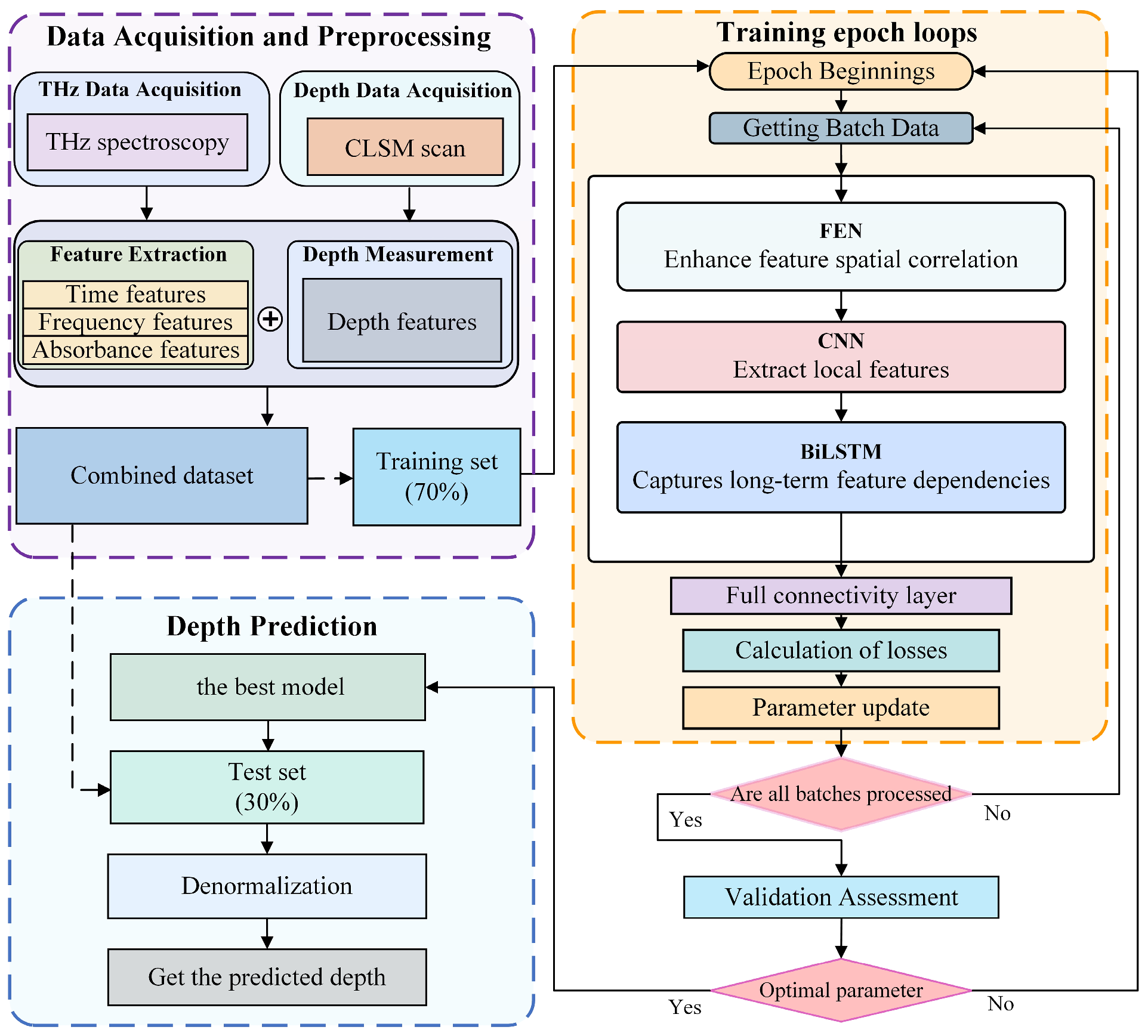
4.2.4. FEN-CNN-BiLSTM Hybrid Model

In this study, as shown in Figure 8, the specific implementation steps of the data processing workflow for the model are outlined as follows:

• THz data and CLSM depth scanning data were systematically collected. From these datasets, six important features are extracted: time-domain peak time, time-domain peak value, frequency-domain peak intensities, frequency-domain integral areas, absorbance peak intensity, and baseline absorbance. These extracted features were then integrated with corresponding depth labels to construct a comprehensive dataset. The dataset was normalized using the MinMaxScaler method. Finally, the dataset is divided into training set and testing subset at a ratio of 70% and 30%, respectively, to facilitate model development and evaluation.
• The input features of the model are initially processed by the FEN structure, which performs feature enhancement while effectively suppressing noise interference.
• After undergoing FEN processing, the enhanced and recombined features are subsequently output to the CNN module for local features of the signal.
• The features processed by the CNN module are input to the BiLSTM module, which captures inter-feature relationships from both forward and backward directions. Finally, the output of the BiLSTM module is mapped to depth labels through fully connected layers.
• To identify the optimal parameters, the model undergoes rigorous evaluation via cross-validation. The best-performing model is then assessed on a held-out 30% test set to determine its final performance metrics.

4.2.5. Parameter Settings and Evaluation Metrics

In this paper, systematic initialization and parameter optimization were conducted for the proposed hybrid prediction model. For parameter updates, the AdamW optimizer was employed, which integrates the rapid convergence characteristics of the AdamW algorithm with weight decay regularization. This approach aims to enhance the model’s generalization ability while effectively preventing overfitting. Various parameters of the hybrid model were fine-tuned and retrained through an iterative process. The initial learning rate was set to 0.001, a value widely adopted as a standard benchmark in deep learning applications. The maximum number of training epochs was set to 500, with early stopping patience set to 30 epochs. Training was terminated when the R² metric during cross-validation failed to improve for 30 consecutive epochs. This configuration was determined after considering the dataset size, model complexity, and training convergence speed. This process ensures that overfitting is avoided in the later stages of training while also preventing premature termination due to random fluctuations, thereby guaranteeing adequate training for the model. The batch size was set to 64, which was determined through preliminary experiments that balanced computational efficiency with model performance.

Regarding the FEN module within the model, its internal structure and parameters were meticulously designed to achieve effective reorganization, denoising, and enhancement of input features. The hidden layer dimension of the FEN module was set to 32, ensuring robust feature representation capability while mitigating the risk of overfitting associated with an excessive number of parameters. During the feature decomposition phase, after multiple experiments, we designed two parallel convolutional pathways, with encoder convolutional kernel sizes of 3 and 5, respectively. This design aimed to capture multi-scale local feature information from diverse receptive fields, with their outputs concatenated to enrich the feature representation. In the channel attention mechanism, the reduction ratio was set to 4, effectively compressing the number of channels, reducing the parameter count, and preserving important inter-channel relationships. In the feature reconstruction stage, the decoder convolutional kernel size was uniformly set to 3 to ensure high-quality feature reconstruction. Within the CNN module, a two-layer convolutional network was constructed. The number of filters in the first convolutional layer was set to 32, while in the second layer it was reduced to 6. The first layer network, equipped with a larger number of filters, fully captures the diversity of input features, whereas the second layer integrates and compresses features by reducing the number of filters, thereby maintaining feature extraction capability while effectively controlling model complexity. Both convolutional layers utilized a kernel size of 3, which achieves an optimal balance between capturing effective local contextual information and controlling computational cost. The unidirectional hidden layer dimension of the BiLSTM module was set to 32. This dimension was carefully selected to balance the model’s capacity for capturing sequence dependencies with the number of parameters, thus mitigating the risk of overfitting. The parameter settings for the FEN-CNN-BiLSTM model are shown in

Table 4. Model parameter settings.

Hyperparameter	Applicable Scope	Value	Remarks
Optimizer	FEN-CNN-BiLSTM	AdamW [30]	Optimization Algorithm of the Model
Initial Learning Rate	FEN-CNN-BiLSTM	0.001	Learning Rate
Epochs	FEN-CNN-BiLSTM	500	Maximum Training Epochs
Batch Size	FEN-CNN-BiLSTM	64	Number of Samples per Training Batch
Loss Function	FEN-CNN-BiLSTM	SmoothL1Loss	Function for Calculating Model Prediction Error
Activation Function	FEN-CNN-BiLSTM	GELU	Activation Function
Hidden Layer Dimension	FEN Layer	32	Feature Dimension of FEN Hidden Layer
Encoder Kernel Sizes	FEN Layer	[3,5]	List of kernel sizes for the two parallel convolutional paths
Attention Reduction Factor	FEN Layer	4	Convolutional Kernel Size
Decoder Kernel Size	FEN Layer	3	Convolutional Kernel Size
Number of Convolutional Layer Filters	CNN Layer	32/6	The first CNN layer uses 32 filters, the second CNN layer uses 6 filters.
Convolutional Kernel Size	CNN Layer	3	Convolutional Kernel Size
Unidirectional Hidden Layer Dimension	BiLSTM	32	Unidirectional Hidden State Dimension

.

These parameter configurations achieve a well-balanced performance in the THz pit depth prediction task, effectively maintaining the model’s expressive capacity while avoiding the risk of overfitting.

To scientifically assess the predictive performance of the model, a comprehensive set of widely recognized metrics is utilized, including Mean Squared Error (MSE), Root Mean Squared Error (RMSE), Mean Absolute Error (MAE), Mean Absolute Percentage Error (MAPE), Coefficient of Determination (R²), and Relative Standard Deviation (RSD) for evaluating the performance of the neural network model.

$$MSE={\displaystyle \frac{1}{n}}\sum _{i=1}^n{\left(y_i-{\widehat{y}}_i\right)}^2,$$

(15)

$$RMSE=\sqrt{MSE},$$

(16)

$$MAE={\displaystyle \frac{1}{n}}\sum _{i=1}^n\left|y_i-{\widehat{y}}_i\right|,$$

(17)

$$MAPE={\displaystyle \frac{1}{n}}\sum _{i=1}^n\left|{\displaystyle \frac{y_i-{\widehat{y}}_i}{y_i}}\right|\times 100\%,$$

(18)

$$R^2=1-{\displaystyle \frac{{\sum }_{i=1}^n{\left(y_i-{\widehat{y}}_i\right)}^2}{{\sum }_{i=1}^n{\left(y_i-{\overline{y}}_i\right)}^2}},$$

(19)

$$RSD={\displaystyle \frac{\sqrt{\frac{1}{n}{\sum }_{i=1}^n{\left(y_i-\frac{1}{n}{\sum }_{i=1}^n{y}_i\right)}^2}}{\frac{1}{n}{\sum }_{i=1}^n{y}_i}}\times 100\%$$

(20)

5. Experimental Analyses

5.1. Model Result Analysis

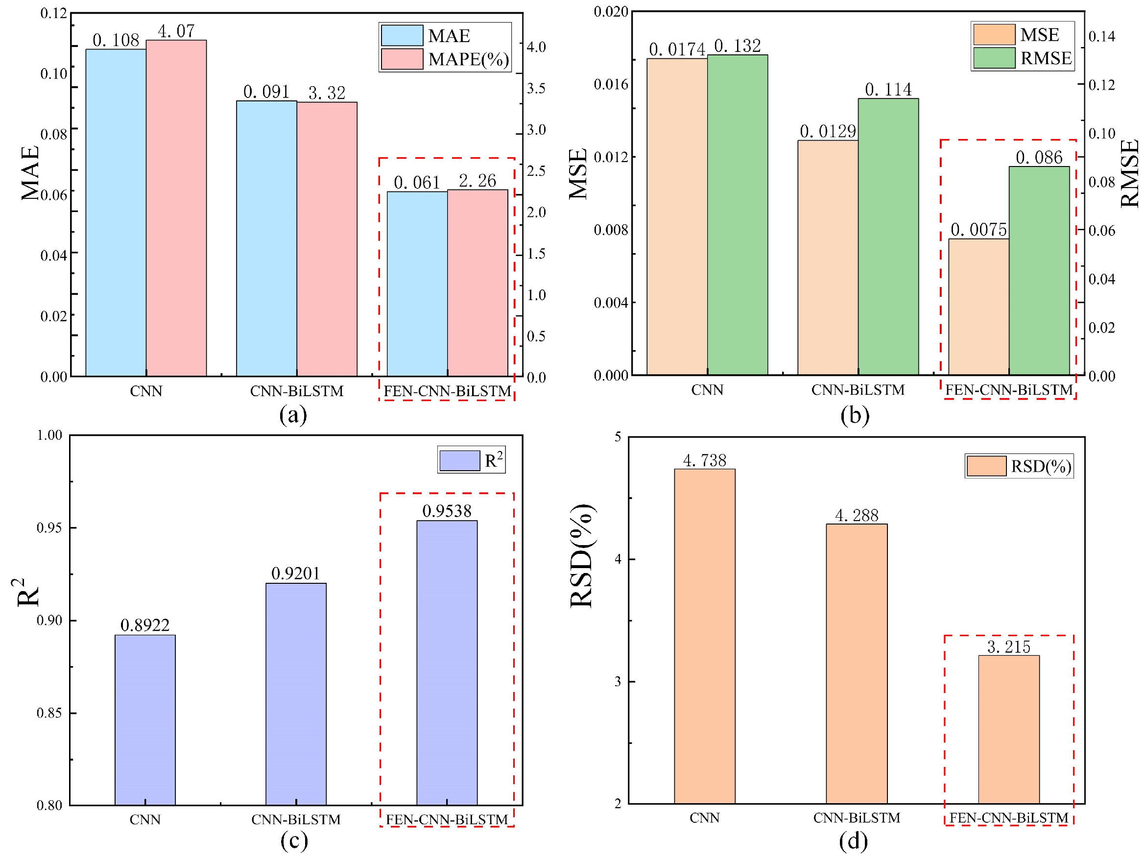
5.1.1. Ablation Experiments

To validate the superiority of the FEN-CNN-BiLSTM model, a series of ablation studies were conducted, comparing the performance of the CNN, CNN-BiLSTM, and FEN-CNN-BiLSTM models. As shown in Figure 9, when compared with the original CNN model in terms of prediction accuracy, the MAE and MAPE of the FEN-CNN-BiLSTM model decreased by 43.08% and 44.4%, respectively. Additionally, the MSE and RMSE decreased by 57.18% and 34.56%, respectively, while the R² metric increased from 0.8923 for the baseline CNN to 0.9539, representing an improvement of 6.90%. In terms of model output stability, the RSD% was reduced by 32.14%. The CNN-BiLSTM model demonstrated an MSE of 0.0129, RMSE of 0.1136, MAE of 0.0941, MAPE% of 3.33%, R² of 0.9202, and RSD% of 4.29%, indicating a significant improvement compared to the standalone CNN model. This enhancement can be attributed to the incorporation of the BiLSTM module, which facilitates a more comprehensive understanding of inter-feature correlations through bidirectional modeling and effectively captures nonlinear relationships among signal features. Nevertheless, its performance metrics still remain inferior to those achieved by the FEN-CNN-BiLSTM model.

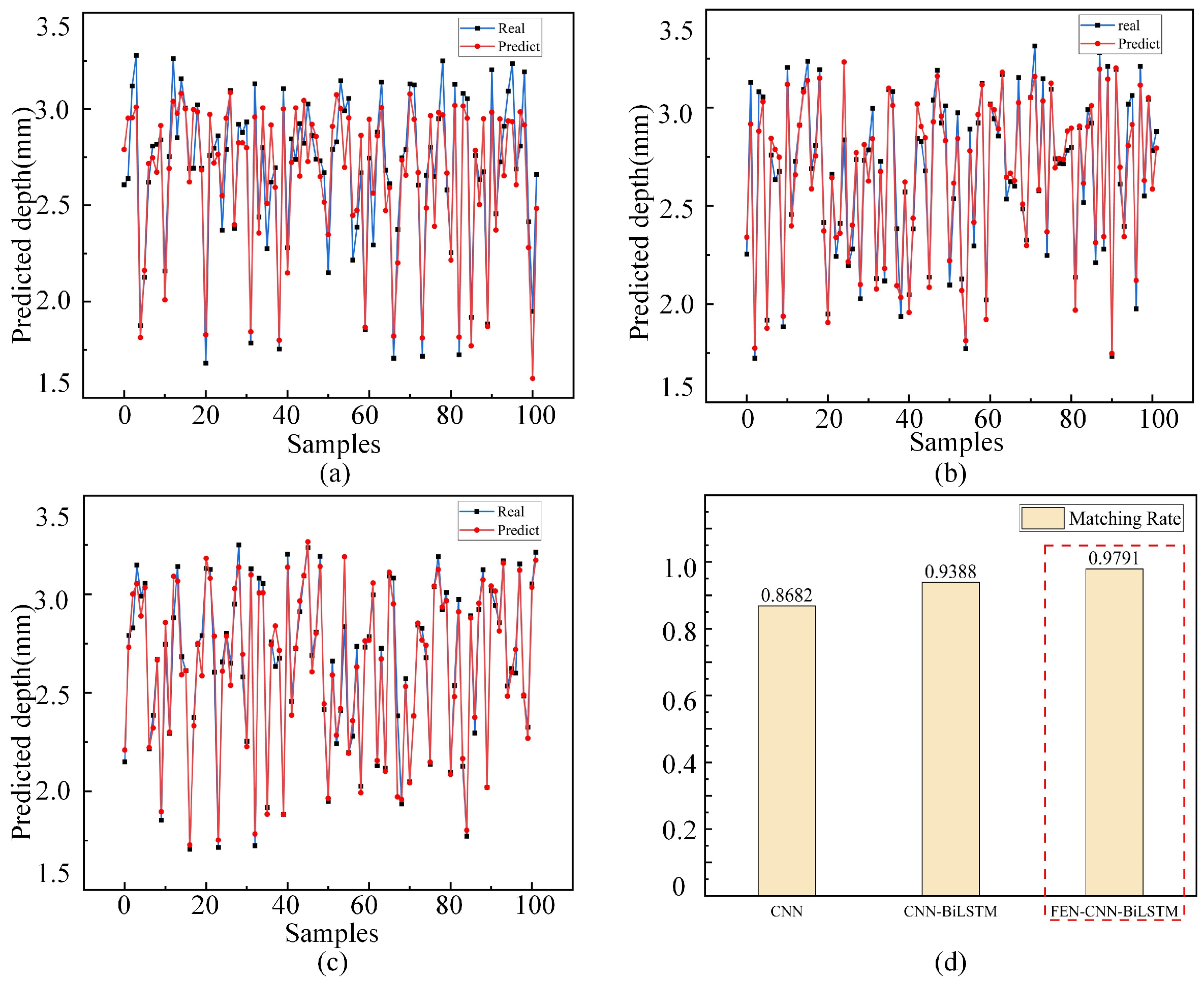
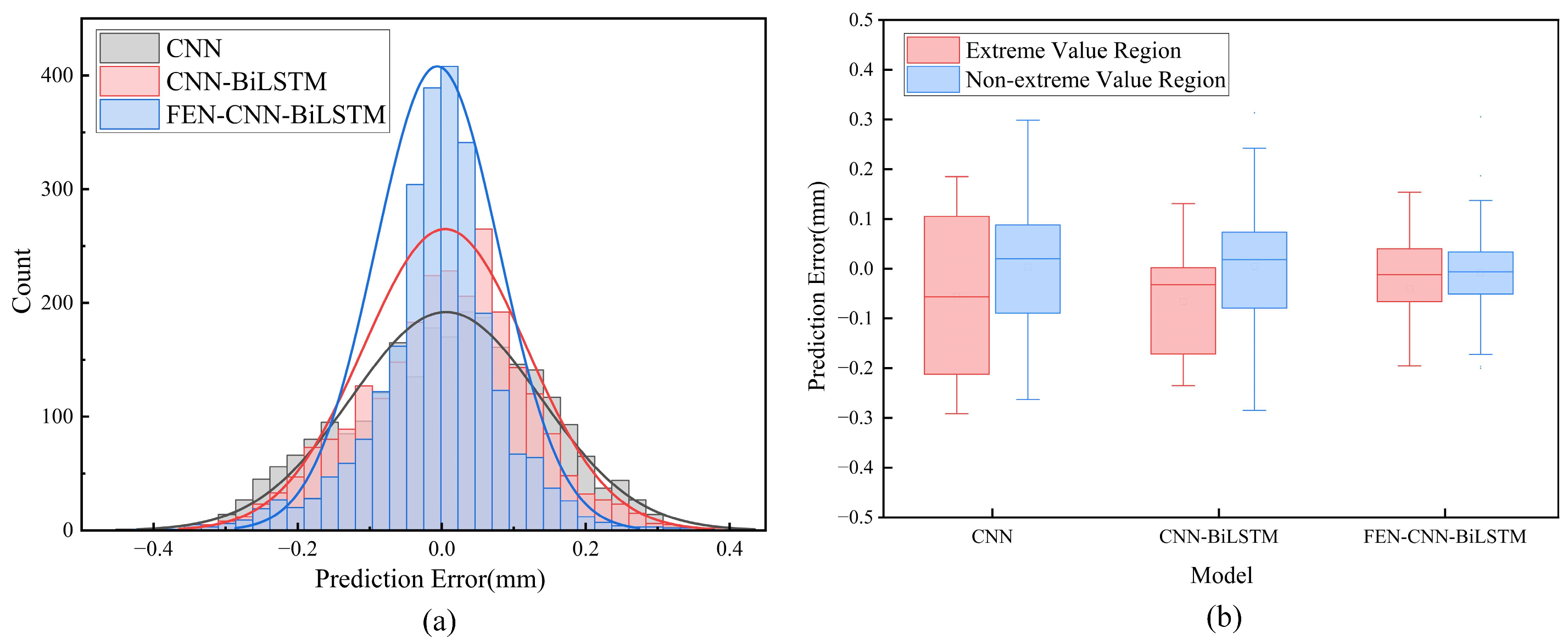
5.1.2. Analysis of Prediction Results

The prediction performances of three models, namely, the multi-feature input CNN neural network, the CNN-BiLSTM neural network, and the FEN-CNN-BiLSTM neural network, on the test set are shown in Figure 10. The results indicate that the prediction generated by the traditional CNN neural network exhibit a low degree of overlap with the true values, revealing substantial deviations, particularly at extremum points. This phenomenon can primarily be attributed to the inherent limitation of CNN in extracting only local feature patterns, which compromises its ability to effectively handling complex correlations among features. Additionally, its inability to reorganize and enhance the original features contributes to suboptimal prediction performance.

The CNN-BiLSTM model demonstrates significant improvement in defect depth prediction. However, considerable errors still exist at extremum points. This indicates that although BiLSTM effectively enhances the correlation of feature, the absence of feature preprocessing results in unmitigated noise, which adversely affects prediction accuracy. Consequently, the expressiveness of the features remains constrained, and the full potential of the BiLSTM module cannot be fully realized. The FEN-CNN-BiLSTM model demonstrates the lowest prediction errors and outperforms other methods across all intervals. This can be attributed to the model’s multi-level processing mechanism. Initially, FEN reorganizes and refines the original features, improving their expressive capability. This enhancement ensures greater model stability, particularly in complex scenarios such as extremum point detection. Subsequently, the CNN extracts local features from the optimized feature set, while BiLSTM network derives more effective temporal correlations.

The histogram presented in Figure 11a clearly indicates that the prediction error distribution of the FEN-CNN-BiLSTM model is more concentrated around the zero value, with a narrower distribution profile. This indicates that the overall deviation of its prediction results from the true values is smaller and exhibits greater stability. Conversely, the error distribution of the traditional CNN model is more dispersed, particularly showing higher frequencies in larger error ranges. Although the CNN-BiLSTM model shows improvement, its error concentration remains less effective compared to the FEN-CNN-BiLSTM model. To further evaluate the model’s performance across different data distribution segments, this study categorizes samples with the smallest 5% and largest 5% of true values as the extreme value region, while the remaining 90% of samples are classified as the non-extreme value region. The statistical analysis presented in Figure 11b shows that as the model improves, the errors in both the extreme value region and the non-extreme value region decrease, and the difference between them also diminishes.

This hierarchical feature processing strategy integrates the advantages of three levels: feature reorganization and enhancement, local pattern extraction, and bidirectional correlation modeling. As a result, the model achieves a more comprehensive understanding and expression of feature information, which in turn enables it to predict depth values with greater accuracy. The experimental results confirm the rationality of the proposed improvement path: progressing from the basic CNN to CNN-BiLSTM, and ultimately to FEN-CNN-BiLSTM, the model demonstrates incremental performance improvements, demonstrating the superiority of the proposed model.

5.2. Comparative Analysis

For further investigation,

Table 5. Comparative experimental results of various models.

Model	MSE	RMSE	MAE	MAPE%	R2	RSD%	FLOPs	Params
Decision Tree	0.021558	0.14683	0.11793	4.4308	0.8667	4.8291
RNN	0.018962	0.1377	0.11606	4.3592	0.8827	5.1373	21.776K	3.265K
MLP	0.019198	0.13856	0.11774	4.4281	0.8813	4.8291	17.280K	17.537K
CNN	0.017421	0.13199	0.10755	4.0668	0.8923	4.7381	25.856K	8.039K
CNN-transformer	0.013398	0.11575	0.09524	3.6029	0.9131	3.8492	80.704K	13.633K
CNN-RESNET	0.013575	0.11651	0.0946	3.6987	0.916	3.6585	310.016K	51.009K
CNN-BiLSTM	0.012907	0.11361	0.09141	3.3288	0.9202	4.2886	194.664K	32.919K
FEN-CNN-BiLSTM	0.00746	0.08637	0.06122	2.2611	0.9539	3.2153	266.416K	43.809K
CNN-BilLSTM-Attention	0.01174	0.10835	0.08162	3.0567	0.9274	4.0038	238.584K	34.892K
CNN-BilLSTM-Transformer	0.008541	0.09242	0.07059	2.6351	0.9472	3.4492	247.216K	41.875K
ResNet-CNN-BiLSTM	0.010873	0.10427	0.08149	3.0257	0.9328	3.8909	364.256K	104.289K
ECA-CNN-BiLSTM	0.011787	0.10857	0.08518	3.1733	0.9271	4.0491	237.564K	38.634K
SelfAttention-CNN-BiLSTM	0.011597	0.10721	0.08278	3.1313	0.9226	4.0226	242.254K	37.757K

presents the performance metrics derived from comparative experiments conducted using various models on the dataset.

As shown in Table 5, the FEN-CNN-BiLSTM model exhibits superior performance across all evaluation metrics. A detailed analysis and discussion are presented below.

In terms of prediction accuracy, the FEN-CNN-BiLSTM model exhibits excellent performance with an MSE of 0.0075, RMSE of 0.0864, MAE of 0.0612, and MAPE of 2.26%. These metrics represent the lowest values among all models, thereby indicating the highest level of accuracy. Furthermore, regarding the model’s fitting capability, R² serves as a critical indicator for measuring the goodness-of-fit. A value closer to 1 suggests a stronger explanatory power of the model. The FEN-CNN-BiLSTM model achieves an R² value of 0.9539, which is the highest among all evaluated models. This result not only confirms the model’s excellent fitting ability but also highlights its ability to effectively capture the main variation patterns in the data.

In terms of model stability, the RSD% serves as a key indicator for measuring the dispersion of prediction results and reflects the consistency of the model’s output. The RSD% of CNN-BiLSTM is 4.29%, which is slightly higher compared to CNN-ResNet and CNN-Transformer. However, when considering overall performance, the CNN-BiLSTM model demonstrates superior results in key accuracy metrics, including MSE, RMSE, MAE, MAPE%, as well as R² fitting capability. This indicates its enhanced prediction accuracy and robust fitting capability. In practical applications, especially in related tasks, such as impact damage depth prediction, prediction precision often takes precedence over the degree of dispersion in the prediction results. Therefore, the CNN-BiLSTM architecture establishes a solid foundation for subsequent model improvements. In contrast, the FEN-CNN-BiLSTM model achieves an RSD% of only 3.22%, which not only indicates its high accuracy but also underscores the superior repeatability and reliability in its prediction results, further demonstrating the model’s stability. By comparison, other models exhibit higher RSD% values, suggesting greater variability in their predictions and relatively inferior reliability and consistency. Although some advanced attention mechanisms, such as the ResNet-CNN-BiLSTM and CNN-BiLSTM-Transformer models, have demonstrated commendable accuracy and stability, their performance is not superior when compared to the FEN-CNN-BiLSTM model, and there is no significant difference in FLOPs and parameter counts. Therefore, it can be concluded that the FEN-CNN-BiLSTM model achieves a better balance among prediction accuracy, stability, and computational efficiency.

Figure 12 illustrates a stability versus goodness-of-fit comparison diagram, where the horizontal axis (R²) represents the model’s prediction performance metric and the vertical axis (RSD%) represents the model’s stability. A higher R² value corresponds to superior prediction accuracy, whereas a lower RSD% value reflects greater stability. As can be observed, the FEN-CNN-BiLSTM model is located in the lower-right region, representing optimal performance, and significantly outperforming other comparative models. These findings indicate that the proposed FEN-CNN-BiLSTM deep learning model exhibits significant advantages in both prediction accuracy and stability compared to the other alternative models.

5.3. External Dataset Verification Experiment

To evaluate the generalization capability and application potential of the proposed FEN-CNN-BiLSTM model, the study introduced an independent dataset for external validation, which was derived from the original dataset. Given the constraints imposed by airworthiness requirements that prevent direct experimentation on the surfaces of in-service aircraft, this study utilized actual damaged samples obtained from a professional laboratory for external validation. The sample materials comprised aircraft skin specimens with impact damage, from which 2215 terahertz spectral data points and corresponding depth labels were systematically collected. The experiment utilized the optimal model selected through cross-validation experiments for testing, obtaining the depth prediction results of the damage.

Table 6. External dataset metrics.

Model	MSE	RMSE	MAE	MAPE (%)	R2	RSD%
FEN-CNN-BiLSTM	0.010365	0.10181	0.07568	2.82620	0.93879	3.8171

shows the prediction performance of the FEN-CNN-BiLSTM model on the external dataset. Despite the accuracy metrics being slightly lower than those obtained from the test results on the original dataset, the model still demonstrated excellent prediction capabilities, reflecting its generalization ability.

6. Conclusions

In this study, we confirm the reliability of utilizing multi-feature spectral characteristics from THz time-domain, frequency-domain, and absorbance for quantitatively assessing the depth of low-velocity impact damage in civil aircraft CFRP. These characteristics are further combined with CLSM depth ground truth labels to construct a multi-feature dataset. The primary contribution of this study is the development and validation of the FEN-CNN-BiLSTM deep learning model. Within this model, the FEN module facilitates feature reorganization and enhancement. After local features are extracted via CNN, these features are subsequently output to BiLSTM for learning inter-feature relationships, improving the robustness of the model.

Results from ablation experiments and comparative analyses indicate that the proposed model consistently outperforms other conventional models across key evaluation metrics, including MSE, RMSE, MAE, MAPE, R², and RSD. It exhibits strong adaptability to defects of varying depths and maintains stable prediction performance under complex conditions at various locations, demonstrating its high robustness. Additionally, the innovative incorporation of regression prediction into THz impact damage detection for civil aircraft CFRP structural safety not only enriches the theoretical system of THz non-destructive testing technology but also provides an effective method for the precise evaluation of low-velocity impact damage in CFRP materials, thus validating its feasibility and engineering practical value. Nonetheless, the primary focus of this study is on low-velocity impact damage. Further investigation is warranted regarding the model’s robustness under extreme impact energy levels, which represents a key area for future research and constitutes one of the current limitations. Future research will focus on integrating a broader variety of carbon fiber damage types and utilizing multimodal data to investigate the extensive application potential of the FEN-CNN-BiLSTM model in complex scenarios. A critical future direction will involve expanding the diversity of the dataset to enhance the model’s generalization ability under a wider range of impact energy levels and under noisy environmental conditions. Additionally, adapting this methodology to other materials or damage modes while simultaneously optimizing model complexity for real-time or embedded applications is essential for maximizing its practical utility.

References

1. Xu, X.; Peng, G.; Zhang, B.; Shi, F.; Gao, L.; Gao, J. Material performance, manufacturing methods, and engineering applications in aviation of carbon fiber reinforced polymers: A comprehensive review. Thin-Walled Struct. 2024, 209, 112899. [Google Scholar] [CrossRef]
2. Li, J.; Su, X.; Wang, F.; Zhang, D.; Wang, Y.; Song, H.; Xu, J.; Guo, B. Effect of laser processing parameters on the quality of titanium alloy cladding layer on carbon fiber-reinforced polymer. Polymers 2025, 17, 1195. [Google Scholar] [CrossRef]
3. Chua, C.Y.X.; Liu, H.-C.; Trani, N.D.; Susnjar, A.; Ho, J.; Scorrano, G.; Rhudy, J.; Sizovs, A.; Lolli, G.; Hernandez, N.; et al. Carbon fiber reinforced polymers for implantable medical devices. Biomaterials 2021, 271, 120719. [Google Scholar] [CrossRef]
4. Zhang, J.; Lin, G.; Vaidy, U.; Wang, H. Past, present and future prospective of global carbon fibre composite developments and applications. Compos. Part B Eng. 2022, 250, 110463. [Google Scholar] [CrossRef]
5. Parveez, B.; Kittur, M.I.; Badruddin, I.A.; Kamangar, S.; Hussien, M.; Umarfarooq, M.A. Scientific advancements in composite materials for aircraft applications: A review. Polymers 2022, 14, 5007. [Google Scholar] [CrossRef]
6. Chen, L.; Lin, X.; Bai, R.; Zhao, Z.; Guo, Z. Anti-bird-strike behavior of M40J carbon fiber reinforced plastic laminates. Compos. Struct. 2024, 339, 118094. [Google Scholar] [CrossRef]
7. Wang, Z.; Zhao, M.; Liu, K.; Yuan, K.; He, J. Experimental analysis and prediction of CFRP delamination caused by ice impact. Eng. Fract. Mech. 2022, 273, 108757. [Google Scholar] [CrossRef]
8. Chen, S.Y.; van de Waerdt, W.; Castro, S.G.P. Design for bird strike crashworthiness using a building block approach applied to the Flying-V aircraft. Heliyon 2023, 9, e14723. [Google Scholar] [CrossRef] [PubMed]
9. Tao, Y.H.; Fitzgerald, A.J.; Wallace, V.P. Non-contact, non-destructive testing in various industrial sectors with terahertz technology. Sensors 2020, 20, 712. [Google Scholar] [CrossRef]
10. Wu, Y.Q.; Chen, M.Y.; Dai, Z.J. Review on the terahertz transmission devices and their applications: From metal waveguides to terahertz fibers. Opt. Laser Technol. 2025, 183, 112339. [Google Scholar] [CrossRef]
11. Amenabar, I.; Lopez, F.; Mendikute, A. In introductory review to THz non-destructive testing of composite mater. J. Infrared Millim. Terahertz Waves 2013, 34, 152–169. [Google Scholar] [CrossRef]
12. Bauer, M.; Friederich, F. Terahertz and millimeter wave sensing and applications. Sensors 2022, 22, 9693. [Google Scholar] [CrossRef]
13. Zhang, J.Y.; Yang, X.K.; Ren, J.J.; Li, L.J.; Zhang, D.D.; Gu, J.; Xiong, W.H. Terahertz recognition of composite material interfaces based on ResNet-BiLSTM. Measurement 2024, 233, 114771. [Google Scholar] [CrossRef]
14. Nüßler, D.; Jonuscheit, J. Terahertz based non-destructive testing (NDT) making the invisible visible. Tech. Mess 2021, 88, 199–210. [Google Scholar] [CrossRef]
15. Zhong, M.; Xu, H.X.; Li, F.; Yang, M.; Li, S.Q.; Lei, X.; Tu, X.G.; Wang, Z.Q.; Li, C.; Zhao, X.; et al. Nondestructive testing and predictability of microcracks in carbon fiber-reinforced composites via terahertz time-domain spectroscopy. Russ. J. Nondestruct. Test. 2024, 60, 96–103. [Google Scholar] [CrossRef]
16. Li, R.; Ye, D.; Zhang, Q.K.; Xu, J.F.; Pan, J.B. Nondestructive evaluation of thermal barrier coatings’ porosity based on terahertz multi-feature fusion and a machine learning approach. Appl. Sci. 2023, 13, 8988. [Google Scholar] [CrossRef]
17. Wang, Q.; Liu, Q.H.; Xia, R.C.; Zhang, P.T.; Zhou, H.B.; Zhao, B.Y.; Li, G.Y. Automatic defect prediction in glass fiber reinforced polymer based on THz-TDS signal analysis with neural networks. Infrared Phys. Technol. 2021, 115, 103673. [Google Scholar] [CrossRef]
18. Zhang, Z.H.; Peng, G.Z.; Tan, Y.P.; Pu, T.J.; Wang, L.M. THz wave detection of gap defects based on a convolutional neural network improved by a residual shrinkage network. CSEE J. Power Energy Syst. 2020, 9, 1078–1089. [Google Scholar] [CrossRef]
19. Zhang, J.; Li, W.; Cui, H.L.; Shi, C.C.; Han, X.H.; Ma, Y.T.; Chen, J.D.; Chang, T.Y.; Wei, D.S.; Zhang, Y.M.; et al. Nondestructive evaluation of carbon fiber reinforced polymer composites using reflective terahertz imaging. Sensors 2016, 16, 875. [Google Scholar] [CrossRef]
20. Zhou, C.L.; Lin, H.J.; Jia, X.L.; Yang, Z.; Zhang, G.; Xia, L.; Li, X.; Li, M.L. Impact morphology characteristics and damage evolution mechanisms in CFRP laminates for hydrogen storage cylinders. Int. J. Hydrogen Energy 2024, 77, 110–125. [Google Scholar] [CrossRef]
21. Yang, S.H.; Kim, K.B.; Oh, H.G.; Kang, J.S. Non-contact detection of impact damage in CFRP composites using millimeter-wave reflection and considering carbon fiber direction. NDT E Int. 2013, 57, 45–51. [Google Scholar] [CrossRef]
22. Yu, Y.; Zhang, Z.H.; Zhang, T.Y.; Zhao, X.Y.; Chen, Y.; Cao, C.; Li, Y.; Xu, K.K. Effects of surface roughness on terahertz transmission spectra. Opt. Quantum Electron. 2020, 52, 240. [Google Scholar] [CrossRef]
23. Kumar, V.; Cecconi, V.; Cutrona, A.; Peters, L.; Olivieri, L.; Gongora, J.S.T.; Pasquazi, A.; Peccianti, M. Terahertz microscopy through complex media. Sci. Rep. 2025, 15, 11706. [Google Scholar] [CrossRef]
24. Koch, M.; Mittleman, D.M.; Ornik, J.; Castro-Camus, E. Terahertz time-domain spectroscopy. Nat. Rev. Methods Primers 2023, 3, 48. [Google Scholar] [CrossRef]
25. Zhang, Z.H.; Huang, Y.; Zhong, S.C.; Lin, T.L.; Zhong, Y.J.; Zeng, Q.M.; Nsengiyumva, W.; Yu, Y.J.; Peng, Z.K. Time of flight improved thermally grown oxide thickness measurement with terahertz spectroscopy. Front. Mech. Eng. 2022, 17, 49. [Google Scholar] [CrossRef]
26. Neu, J.; Schmuttenmaer, C.A. Tutorial: An introduction to terahertz time domain spectroscopy (THz-TDS). J. Appl. Phys. 2018, 124, 231101. [Google Scholar] [CrossRef]
27. Wang, Q.F.; Wang, Q.C.; Yang, Z.F.; Wu, X.; Peng, Y. Quantitative analysis of industrial solid waste based on terahertz spectroscopy. Photonics 2022, 9, 184. [Google Scholar] [CrossRef]
28. Makhloughi, F. Artificial intelligence-based non-invasive bilirubin prediction for neonatal jaundice using 1D convolutional neural network. Sci. Rep. 2025, 15, 11571. [Google Scholar] [CrossRef] [PubMed]
29. Liu, M.; Wang, X.H.; Zhong, Z.W. Ultra-short-term photovoltaic power prediction based on BiLSTM with wavelet decomposition and dual attention mechanism. Electronics 2025, 14, 306. [Google Scholar] [CrossRef]
30. Xiong, L.; Su, L.; Zeng, S.; Li, X.; Wang, T.; Zhao, F. Generalized spatial–temporal regression graph convolutional transformer for traffic forecasting. Complex Intell. Syst. 2024, 10, 7943–7964. [Google Scholar] [CrossRef]
Figure 1. Imaging analysis under various parameters (a) Time-domain imaging; (b) Frequency-domain imaging; (c) Absorbance imaging.
Electronics 14 02412 g001
Figure 2. CLSM 3D morphology and depth layers (a) Damaged specimen (b) Top view of the damaged region (c) Front-side view of the damaged region (d) Oblique top view.
Electronics 14 02412 g002
Figure 3. THz time-domain analysis (a) Imaging map with measurement points L1–L5 (b) Time domain spectra showing peaks P1–P5 (c) Peak time (d) Peak intensity.
Electronics 14 02412 g003
Figure 4. THz frequency-domain analysis (a) Imaging map with measurement points L1–L5 (b) Frequency spectra showing peaks P1–P5 (c) Peak intensity (d) Integral area.
Electronics 14 02412 g004
Figure 5. THz absorbance analysis (a) Imaging map with measurement points L1–L5 (b) Absorbance spectra showing peaks P1–P5 (c) Peak intensity (d) Absorbance baseline.
Electronics 14 02412 g005
Figure 6. Overall flowchart of impact damage depth prediction based on THz multi-features.
Electronics 14 02412 g006
Figure 7. FEN-CNN-BiLSTM model structure.
Electronics 14 02412 g007
Figure 8. Flowchart of the FEN-CNN-BiLSTM hybrid model.
Electronics 14 02412 g008
Figure 9. Comparative analysis of metrics for various optimization algorithms (a) Relative error metrics of various optimization algorithms; (b) Absolute error metrics of various optimization algorithms; (c) Prediction accuracy metrics of various optimization algorithms; (d) Prediction performance metrics of various optimization algorithms.
Electronics 14 02412 g009
Figure 10. Comparative analysis of fitted lines for various optimization algorithms (a) CNN neural network, (b) CNN-BiLSTM network, (c) FEN-CNN-BiLSTM network, (d) Comparison of the degree of overlap of regression fitted lines for various optimization algorithms.
Electronics 14 02412 g010
Figure 11. Error analysis (a) Error histograms of different algorithms, (b) Errors in different regions.
Electronics 14 02412 g011
Figure 12. Comparison of stability and goodness-of-fit for various models.
Electronics 14 02412 g012