Abstract
Global Navigation Satellite Systems (GNSSs) are widely used for positioning, timing, and navigation services. Such widespread usage makes them exposed to various threats including malicious attacks such as spoofing attacks. The availability of low-cost devices such as software-defined radios enhances the viability of performing such attacks. Efficient spoofing detection is of essential importance for the mitigation of such attacks. Although various methods have been proposed for that purpose it is still an important research topic. In this paper, we investigate the spoofing detection method based on the integrated usage of discrete wavelet transform (DWT) and machine learning (ML) techniques and propose efficient solutions. A series of experiments using different wavelets and machine learning techniques for Global Positioning System (GPS) and Galileo systems are performed. Moreover, the impact of the usage of different types of training data are explored. Following the computational complexity analysis, the potential for complexity reduction is investigated and computationally efficient solutions proposed. The obtained results show the efficacy of the proposed approach.
1. Introduction
Global Navigation Satellite Systems (GNSSs) are commonly used today for positioning, timing, and navigation services. Given their widespread use, these systems are highly susceptible to various threats, with spoofing attacks being the most frequent type. A spoofing attack is based on the transmission of fake signals in order to deceive the receiver and take over its navigation system. Since the power of the received satellite signal is very weak, due to the influence of radio frequency interference, it can lead to the reduced accuracy of positioning and timing or even to a complete lack of a navigation solution. The weak power of the received signal is the reason why the receiver takes the signals with higher power and calculates its position based on them.
Such attacks are relatively easy to carry out due to the availability of low-cost equipment. A single software-defined radio (SDR), such as HackRFOne, is sufficient to perform simple spoofing attacks, posing a significant threat. The devices that are most vulnerable to spoofing attacks are smartphones which are mostly used for navigation services nowadays. Increased attention has been paid to these attacks in the open literature since the authors in [1] developed a portable GPS spoofer. Using GNSS receivers that are resistant to spoofing attacks is key to secure positioning, navigation, timing, and synchronization. Therefore, effective spoofing attack detection and signal-type classification become extremely important.
Although various detection methods have been proposed, it is still an important topic of research. Some of the methods for detecting these attacks that are still in their infancy in the field of GNSS and have not been sufficiently investigated are radio frequency fingerprinting (RFF) methods. The main motivation of this paper was to investigate the RFF discrete wavelet transform (DWT) in combination with machine learning classifiers for effective spoofing detection and signal-type classification. The discrete wavelet transform is used for spoofing detection because it has the ability to localize information in the time–frequency domain, which is particularly useful for detecting anomalies such as fake signals or abnormal patterns. Spoofing attacks often change the structure of the signal only in certain time segments and the discrete wavelet transform enables their detection because it segments the signal into time–frequency components. Approximation and detail DWT coefficients contain compact information about the energy and frequency components of the signal, and it is easy to calculate statistical, spectral, and texture features which are used as input data in classifiers. Another advantage of this approach is using Daubechies db4 and db8 wavelets that have very good localization in time and frequency, which provides resistance to noise. Compared to other types of wavelets (e.g., Haar, Symlet), Daubechies wavelets retain more energy of the signal in the approximation coefficients, resulting in more accurate statistical and texture features. This increases the discriminative power of the features used for classification. The DWT has a lower computational complexity compared to e.g., the Wigner–Wille transform, which allows a faster implementation in real-time GNSS receivers. This paper aimed to compare different machine learning classifiers using different types of input classification data and to predict the type of signal with high accuracy. Furthermore, using the pre-extracted features for the input data reduces the computational complexity of the proposed approach. This paper proposes an integrated approach based on the combination of discrete wavelet transform (Daubechies db4 and db8 wavelets) and machine learning models for intermediate spoofing attack detection and signal-type classification. The approach is applied to both GPS and Galileo systems. The performance of each machine learning model based on different types of input classification data and computational complexity is compared.
This paper and all presented results are the result of doctoral research. The methodology and part of the results were taken from the doctoral dissertation [2].
The main contributions of this paper are:
- The application of different types of wavelets including db4 and db8 and one-level decomposition of images obtained by using the discrete wavelet transform on Oak Ridge Spoofing and Interference Test Battery (OAKBAT) GPS and Galileo datasets in static scenarios for GNSS spoofing detection.
- The detection of fake signals and classification of signal type using an integrated approach based on the discrete wavelet transform and machine learning models.
- The comparison of the performance of machine learning models using different types of input classification data.
- Reducing the computational complexity of the proposed approach by using pre-extracted classification input data.
This paper is organized as follows. The Section 1 gives an introduction, motivation, and the aim of the research. The Section 2 provides an overview of the methods for detecting spoofing attacks that have been explored so far. In Section 3, the proposed methodology used in our research is presented. The Section 4 presents the results obtained by using the proposed approach, while Section 5 brings conclusions.
2. Related Works
As positioning and navigation services are available in nearly all devices, including the smallest ones, timely detection of spoofing attacks is crucial to prevent undesirable consequences. There are numerous methods for spoofing attacks detection. The simplest is the traditional method, which monitors signal strength. This approach is often employed for quick response to attacks and forms the foundation of many other spoofing detection methods [3].
Other widely used methods include data bit-based techniques such as tracking and analyzing National Marine Electronics Association (NMEA) messages [4], comparing the Time of Arrival (ToA) [5], and monitoring the Direction of Arrival (DoA) [6]. Signal processing techniques include power-based methods [7], antenna-based methods [8], and correlation peak monitoring [9,10]. A comprehensive overview of spoofing detection methods and countermeasures is provided in the survey paper [11].
Machine learning and deep learning approaches have recently become the most popular techniques for detecting GNSS spoofing attacks. Various studies analyze the effectiveness of different machine learning methods. The authors in [12] demonstrate that classification and regression decision tree models outperform other machine learning approaches for GPS signal classification. Similarly, the results in [13] show that support vector machines (SVMs) provide superior results for detecting spoofing attacks. However, [14] compares several machine learning methods and finds that k-nearest neighbors (KNN) outperforms SVMs. Results in [14,15], and [16] confirm that the SVM method is a reliable approach for identifying fake signals. A multi-parameter detection method proposed by Chen et al. [16] significantly enhances spoofing detection compared to traditional methods. Neural Networks (NN), as a deep learning approach, are also commonly utilized, as shown in [17,18,19].
While recent developments have introduced a variety of spoofing detection methods, significant research is still being dedicated to exploring and developing innovative techniques. One method that remains relatively unexplored in the GNSS context is the radio frequency fingerprinting method. This method distinguishes between authentic and fake signals by analyzing unique signal characteristics to detect inconsistencies indicative of spoofing attacks. RFF techniques are widely applied in various domains, including Wi-Fi, the Internet of Things, and cellular networks, as presented in [20,21,22,23,24].
However, limited research is available on using RFF methods in the GNSS field. Investigations of different RFF approaches are presented in [25]. A review of RFF techniques for GNSS spoofing detection and a method for pre-correlation spoofing detection using RFF is presented in [26]. The proposed approach involves feature identification, extraction, data pre-processing, and the application of machine and deep learning classifiers (i.e., SVM, KNN, CNN). The presented findings indicate that combining various features within the SVM model yields the best results. In [27], support vector machines (SVMs) and logistic regression are utilized to classify radio frequency (RF) fingerprints (features), determining whether a signal is genuine or counterfeit, achieving an accuracy exceeding 90%. Similarly, in [28], an SVM is applied to three datasets for pre- and post-correlation [29] classification of authentic and fake signals. The findings indicate that classification in the pre-correlation domain yields higher accuracy (99.99%) compared to the post-correlation domain (87.72%). The reason for this difference lies in the additional filter processing in the post-correlation domain, which complicates the discrimination of fingerprints. An optimized random forest model is used in [30] for fake signal detection in the TEXBAT dataset with a classification accuracy of 99.7%.
The framework proposed in [31] for spoofing detection within the post-correlation domain relies on a convolutional autoencoder. This framework is validated through experiments using the Texas Spoofing Test Battery (TEXBAT) dataset, a benchmark in GNSS spoofing detection research [32]. TEXBAT is also employed by [33] to validate the Signal Quality Monitoring (SQM) technique, which assesses the quality of the correlation function peak under realistic spoofed conditions. Finally, ref. [34] introduces a GNSS spoofing detection method based on simulations under ideal conditions for RFF identification. That approach extracts RF fingerprints from incoming signals using deep learning, eliminating the need for manual feature selection. Two deep learning-based classification methods for RFF identification are compared: one focuses on analyzing the signal’s physical layer characteristics, while the other works in a way that extracts RFF in the time–frequency domain. Both techniques demonstrate high effectiveness in spoofing detection.
The authors in [35] investigate the use of convolutional neural networks (CNNs) for classifying various unintentional interference signals while excluding spoofing attacks. The proposed method demonstrates high effectiveness in two scenarios: ground-station monitoring and classification via low Earth orbit (LEO) satellites, achieving 99.69% accuracy even for low-power interference and enabling real-time monitoring of jammers. Inputs to the CNN include time–frequency visual representations of raw samples and derived statistical metrics. The methodology employs signal analysis using the short-term Fourier transform (STFT) and Wigner–Ville transform and evaluates two CNN architectures, AlexNet and ResNet, in terms of accuracy, F1-score, inference time, and model size. That work extends prior research by integrating extracted features to enhance classification performance, particularly for low-power signals, and classifies multiple interference types. The method proves efficient for real-time applications in GNSS interference detection.
According to the state of the literature and to the authors’ knowledge, different types of Daubechies wavelets db4 and db8 in combination with machine learning models and different types of classification data for spoofing detection have not been proposed yet. Similar approach is presented in [35] for jamming detection and classification of different jamming types based on a CNN and Wigner–Ville transform, which is computationally more complex than a DWT.
This paper proposes an approach for spoofing attack detection and signal-type classification based on the combination of discrete wavelet transform and machine learning classifiers. Furthermore, the authors in this research aim to reduce the computational complexity by using pre-extracted features for the classification. All results in this paper are presented for approximation coefficients on decomposition level 1 and for the SVM model, since the SVM shows the best performance for both types of wavelets.
3. Methodology
This section presents the proposed approach used for spoofing attack detection. The approach is based on the combination of discrete wavelet transform and machine learning classifiers. The key components of the methodology are outlined below.
3.1. Proposed Approach
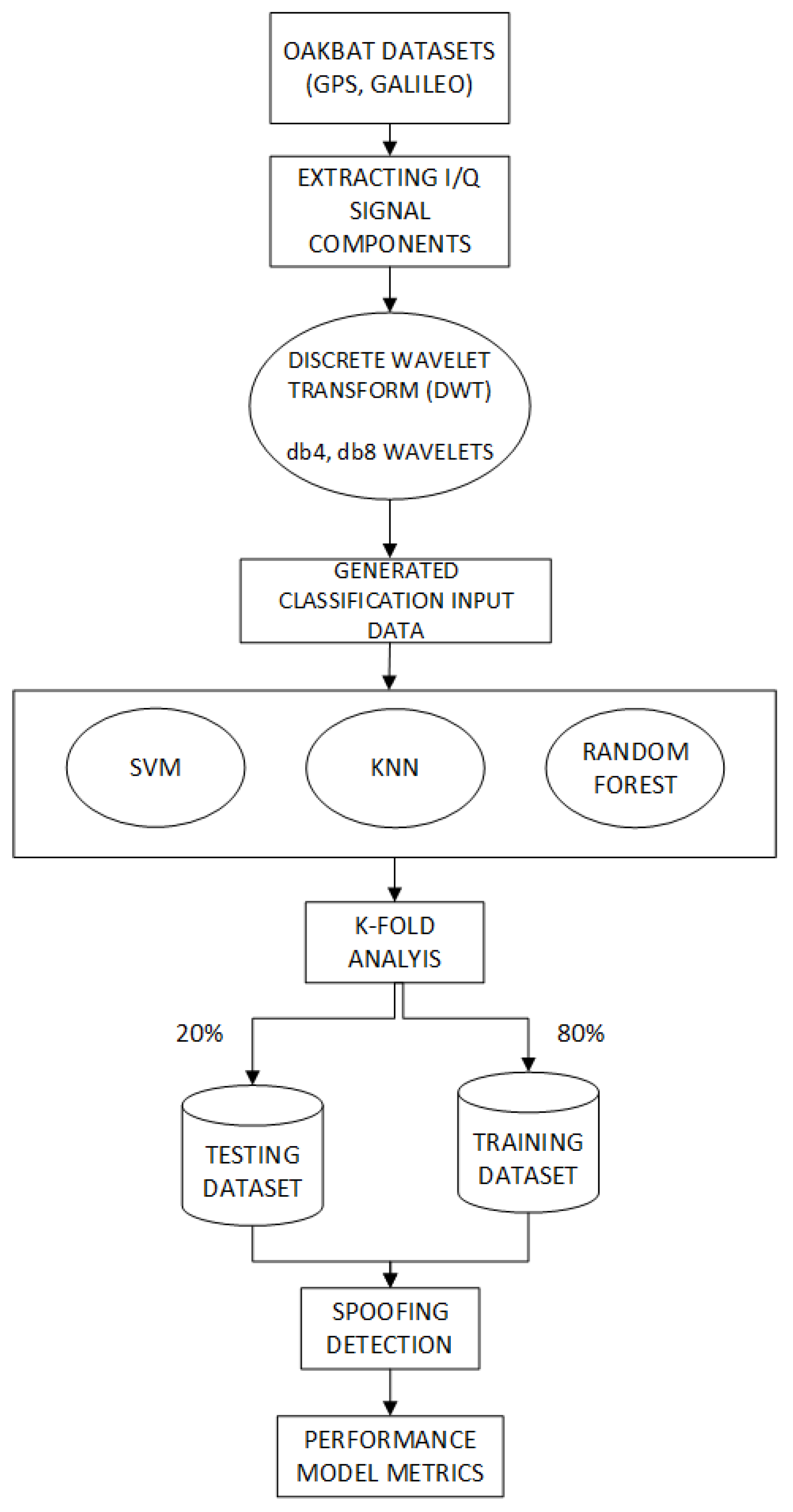
The proposed integrated approach consists of two steps: (1) the application of the discrete wavelet transform to selected datasets, (2) the application of selected machine learning models to the generated datasets. Figure 1 shows the block diagram of the proposed approach. Firstly, in-phase and quadrature (I/Q) components are extracted from each OAKBAT dataset. The data are split into segments to facilitate the implementation of the algorithm’s calculations on limited resources. After that, a level 1 discrete wavelet transform is applied to the I/Q components, and four types of coefficients (approximation, horizontal, vertical, and diagonal) are extracted. As a result of the first step, the generated datasets based on different types of input classification data are obtained. Three types of generated data (images, spectral and statistical features, and image processing and texture analysis features) are used as the input data in machine learning classifiers, including SVM, KNN, and RF. k-Fold cross-validation is applied on all machine learning models. The result of the second step is a signal-type classification (class/output of the model), hence the model return as output whether the signal is authentic or fake. All models are evaluated using standard model performance parameters such as confusion matrix, accuracy, precision, recall, and F1-score.
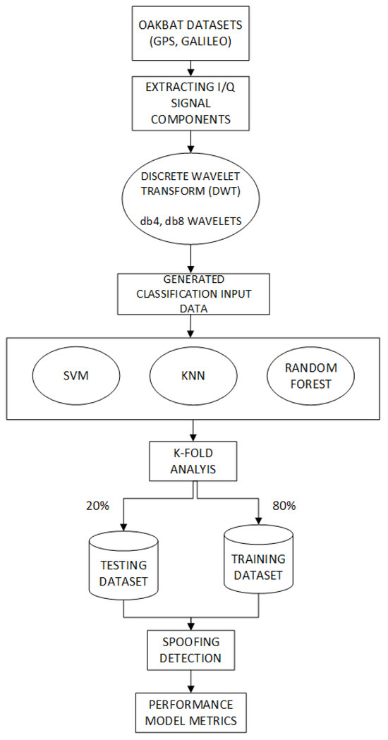
Figure 1.
Block diagram of the proposed approach.
3.2. Implementation Details and OAKBAT Datasets
The experimental part was performed in the software package Matlab R2024a by using the following three toolboxes: Signal Processing, Wavelet Toolbox, and Statistics and Machine Learning Toolbox. The following parameters were used in the DWT: a decomposition level of 1, the optimal duration of the signal segment was 4 ms, the number of segments per iteration was 100, 400 ms of the data was processed during one iteration, and the duration of each OAKBAT dataset was 480 s. Level 1 of the DWT decomposition was used in experiments. The first level of decomposition is the most detailed because it contains the highest frequency components of the signal. As the decomposition depth increases, the temporal resolution of the wavelet coefficients decreases. It means that sudden power jumps or abrupt phase shifts become harder to localize in time because each deeper level effectively doubles the width of the analysis window and reduces the ability to detect short-duration anomalies. Considering this, using the coefficients from level 1 in machine learning classification, as a rule, gives better classification results.
Regarding the machine learning models implementation, in image classification, the bag of features (BoF) selection approach was applied. It means that the model used 70% of the strongest features for classification to improve the quality of the visual vocabulary and reduce the influence of noise. The strongest features contain the most informative parts of the image, such as edges or textures. The weakest features (30%) that may represent noise or unimportant details were eliminated and rejected. Overfitting was reduced by using this BoF approach. In the SVM model, the Gaussian (radial base function—RBF) kernel was chosen for its flexibility and robustness in nonlinear classification problems. This kernel exhibits resistance to noise and is less sensitive to isolated outliers than polynomial kernels, which is crucial in real-world GNSS environments. RBF implicitly handles local variations in signal power, critical for spoofing detection with small dB advantages (e.g., 0.4 dB in os4). In the KNN model, the number of neighbors was set to 5, and we used the Euclidean distance, as these values showed the best model performance. The number of trees was set to 100 and 200 in order to see how the model performed when that number was increased. Also, the built-in validation method, Out-Of-Bag (OOB) prediction, was used in random forests for evaluating the model. Each tree was trained on a random bootstrap sample, and OOB samples were left out and then used for the model evaluation, providing an internal estimate of performance without the need for a separate test dataset. When using more than 200 trees, the performance stabilized with negligible improvements in accuracy. Only the execution time and computational complexity increased with the increase in the number of trees. The model achieved stable and reliable results with 100–200 trees, and adding more trees did not significantly improve accuracy or other metrics. In order to prevent the model overfitting, k-fold cross-validation was applied to all machine learning models. The dataset was divided into k folds, in this research K was 5, and used to assess the model’s ability as new data became available. With this value of K, 80% of the data were used for training, and 20% were used for testing. Since machine learning models used in this research were supervised, data were divided into folders based on the class they belonged to. Folders “real” and “spoofed” denoted the labels and output types used for classification. The predicted variable was the class of the signal (type of the signal): real or spoofed. The class distribution was evenly balanced in each 5-fold cross-validation step because the number of samples per class was equal.
The datasets of digitized radio signals OAKBAT were developed to investigate intermediate spoofing attacks in the GNSS area and are complementary to the TEXBAT datasets. Unlike the TEXBAT datasets, which are based only on GPS system signals, OAKBAT additionally contains Galileo signals, which was an additional reason for using this dataset in this research. OAKBAT consists of 8 datasets containing only GPS L1 C/A signals and 8 datasets containing only Galileo E1 signals. It was created using the commercial GNSS simulator Orolia Vulnerability Test System, which consists of two Orolia GSG-6 series multi-frequency and multi-constellation GNSS simulators. Simulators use the actual broadcast ephemeris data files from NASA Crustal Dynamic Data Information System for GPS and CNES Navigation and Time Monitoring Facility for Galileo. The system used for recording and playback of the recorded files was a software-defined radio Ettus X310. The parameters used to create the OAKBAT dataset were as follows: environment “open sky”, date and time of start of all scenarios: 19 March 2020, 09:59:42 UTC, powers for GPS and Galileo satellites: 123.5 dBm and −125 dBm, sampling frequency 5 MHz, and the data format was int16. The duration of each .bin file is 8 min.
For this research, OAKABAT datasets [36] for GPS and Galileo in static scenarios were used. Those datasets were GPS clean, os2, os3, and os4, which are equivalent to the Galileo clean, os10, os11, and os12 datasets. The difference between these spoofing datasets is in the power level advantage of fake signals in relation to the authentic ones, as shown in Table 1.

Table 1.
OAKBAT datasets with the power level advantage of fake signals.
3.3. Discrete Wavelet Transform
The discrete wavelet transform breaks down a discrete-time signal into wavelets across different scales, capturing both time and frequency information. Unlike the Fourier Transform, which only reveals frequency content, the DWT also provides time localization. This makes it especially useful for analyzing signals that are non-stationary or contain transient features.
In the context of GNSS spoofing detection, the Discrete Wavelet Transform can be utilized to identify signal anomalies that may suggest deceptive activity. Its applications in spoofing detection include the following:
- Decomposing the signal into various frequency components, enabling feature extraction that may indicate spoofing attack.
- Classifying signals as either authentic or fake using machine learning methods.
- Computational efficiency makes it suitable for real-time processing where immediate detection is critical, such as in GNSS receivers.
The following conditions are applied to the wavelets:
- The admissibility condition means that the wavelet function must have zero mean:
- The normalized condition means that the wavelet function has finite energy:
Condition (1) indicates that the wavelet function has equal positive and negative areas so both low and high frequencies can be captured.
The discrete wavelet transform is defined as
where is a wavelet basis function at a specific scale j and shift k for each discrete sample n. The wavelet basis function is created from the mother wavelet
where scale is the normalization factor, is the scale that compresses or spreads the wavelet, moves wavelet in time, j controls the frequency, and shift k controls the translation (position) of the wavelet in time [37,38,39].
The decomposition of discrete signal is performed by using low-pass and high-pass filters to capture both low- and high-frequency components. The results of the decomposition are approximation and detail coefficients at each level. Approximation coefficients are defined with the following equation:
where is the output of low-pass filtering.
Detail coefficients are defined as
where is the output of high-pass filtering.
The original signal may be reconstructed by using approximation and detail coefficients as follows:
In this paper, Daubechies db4 and db8 wavelets were integrated with machine learning methods for spoofing detection and signal-type classification. These wavelets enable the efficient analysis of signal changes in time and frequency (good localization), which is crucial for detecting anomalies that occur during spoofing attacks. Furthermore, both db4 and db8 wavelets have the ability to detect subtle but significant differences between authentic and fake signals. As already stated, Daubechies wavelets retain more energy of the signal in the approximation coefficients, resulting in more accurate statistical and texture features. More accurate features give better classification results.
3.4. Application of Machine Learning Models for Spoofing Attack Detection
As already mentioned, machine learning methods are a reliable and effective approach for the detection of spoofing attacks and the classification of signal types. The machine learning methods used in this paper were support vector machines [13,15,16,26], k-nearest neighbors [9,14,29], and random forest [12,30], since these methods have been validated in recent studies for their effectiveness in GNSS spoofing detection. Due to their high performance in classification tasks with nonlinear features, robust detection of fake signals was achieved. SVM has a robust performance when using kernel functions to handle nonlinear separability. KNN enables the intuitive recognition of similar patterns without the need for model training. As an ensemble model that uses multiple trees, RF gives high accuracy and ensures resistance to noise and overfitting. These methods represent a balance with respect to accuracy, robustness, and scalability for spoofing attack detection.
3.4.1. Support Vector Machine (SVM)
A support vector machine is a supervised machine learning method particularly used for classification and regression. The aim of the SVM method is to find an optimal hyperplane that separates the data points into different classes. An optimal hyperplane is defined as the linear decision function with the maximal margin between the vectors of the two classes [40]. In linearly separable data, SVM successfully finds separators, while in nonlinear separable data, it uses the kernel technique, projecting the data into a higher dimension where it is linearly separable.
The support vector model is the simplest and is represented by the expression [40]
where is the input vector, is the weight vector, and is a free member (bias). Often, the designation b is used instead of the mark. The bias moves the hyperplane to the left or right. If , then the hyperplane always passes through the center of the coordinate system, which can limit the model and reduce its ability to properly separate the data. The boundary between the classes is the hyperplane , which is mathematically defined by the following expression:
The points closest to the margin are called support vectors and meet the following conditions:
The supporting vectors lie on margins at a distance (this expression represents the width of the margin) from the hyperplane. They are important because they affect the limits of decision-making.
The margin represents the distance of the hyperplane to the nearest sample. Since the goal of this method is to obtain the maximum margin, it is necessary to find such a hyperplane that will maximize this distance:
where for each hyperplane (function argmax iterates over all hyperplanes), the minimum distance to the nearest sample is calculated and the hyperplane for which this distance is the greatest is taken. For a hyperplane that maximizes the margin, the patterns on the left and right are equidistant from it.
The final expression for the maximum margin optimization problem, or the so-called quadratic programming problem, is
with the condition
If the data are not linearly separable, the SVM uses a kernel function to map the data into a multidimensional space where it becomes linearly separable. The most commonly used core functions are linear, polynomial, and radial base functions. Once the optimal hyperplane is found, the SVM can be used to classify new data points by checking which side of the hyperplane they are on. In summary, the support vector machine is an effective algorithm which solves complex classification problems by finding the optimal hyperplane that maximizes the margin between classes.
3.4.2. k-Nearest Neighbors (KNN)
The k-nearest neighbors method is an unsupervised machine learning method based on the idea that data patterns belonging to the same class often tend to be spatially close to each other. This technique is used for classification and regression, where the decision on the prediction depends on the k-nearest neighbors, that is, the data points that are closest to the observed sample according to some distance metric, such as the Euclidean distance. The classification is based on the majority vote of the adjacent tags, whereas regression is performed by calculating the average value of the neighbors. The KNN method is computationally simple because it does not require the creation of an explicit model during training, but all data are stored in memory. This is the so-called lazy learning method, which means that the calculations take place only in the prediction phase.
Despite these challenges, the KNN method is frequently used in practice due to its simplicity and intuitiveness [41,42].
The KNN algorithm consists of several steps [43]:
- Select k that defines how many neighbors will be checked to determine the class of a particular data point. For example, if , the instance is assigned to the same class as its nearest neighbor.
- Determine the distance metric. In order to determine which data points are closest to the point for which the class is to be determined, the distance between the observed point and the other data points should be calculated. These distance metrics help form decision boundaries, which divide the question points into different regions. Given the new data point, the algorithm calculates the distance between the new point and all points in the training dataset to find the nearest neighbors of the new data point.
- Based on the calculated distance, k-nearest neighbors are selected. The neighbors are the k training points that are closest to the new data point. In the case of binary classification, the decision boundary is the line that separates the two classes. On the other hand, in the case of a multi-class classification, the boundary is the hyperplane that separates the different classes.
- Assign a class to a new data point. After finding the k-nearest neighbors, the algorithm assigns a new data point to the class that is most common among its k-closest neighbors. In other words, the algorithm uses the majority class k-nearest neighbors as the predicted class for the new data point.
- The algorithm repeats the previous steps for each new data point.
3.4.3. Random Forest (RF)
Random Forest is a popular machine learning method that uses a set of multiple decision trees for classification or regression tasks. The key idea of the method is to combine predictions from different independently generated decision trees to improve model accuracy and reduce the tendency to overfit. Each tree within the forest is trained on different randomly selected subsets of data (bagging method), and during the process of selecting features for individual nodes of the tree, a random subset of features is used, thus reducing the correlation between the trees.
The random forest algorithm consists of several steps [44,45,46]:
- A subset of the same n data is randomly taken from the original dataset, but with repetition, which means that some patterns may appear multiple times while others may be omitted entirely. In this way, the so-called bootstrap pattern is formed, which is used to train one decision tree, thus reducing overtraining (each tree sees only part of the data) and increasing the diversity of the model (each tree learns on a different pattern). This process is repeated for each tree in the model.
- A random subset of m features is selected from a total set of p features. This helps to reduce the correlation between the trees.
- A decision tree is built for each bootstrap pattern and selected features using a specific separation criterion (the previously mentioned Gini impurity and mean mutual information content). The process is repeated until a predetermined stop criterion is met (e.g., maximum tree depth, minimum number of samples per leaf).
- The final prediction (class) of the model is obtained by adding the predictions of all decision trees and is defined aswhere is a finite class, c is the class for which votes are calculated, B is the number of trees in the forest, is a prediction of a single tree for the input data x, and is an indicator function that returns 1 if , otherwise it returns 0 [46].
The random forest algorithm is more resistant to overfitting because it uses more different trees and adds up their decisions. Furthermore, it is good for large datasets, can work with mixed data types (numerical and categorical), and achieves very high accuracy. Bootstrapping allows the RF to build multiple different decision trees, which improves the robustness and accuracy of the model. The disadvantage of this algorithm is the high computational complexity compared to a single tree (more trees = higher computational complexity).
3.5. Model Performance Parameters
Classification models have a discrete output, and parameters that compare discrete classes are needed. The accuracy alone is not sufficient to determine the reliability of the model, and therefore additional performance metrics are used, which are described below.
- A confusion matrix, also known as an error matrix, is a special type of table that allows the performance of an algorithm to be visualized. Each row in the matrix represents patterns in the actual class, and each column represents patterns in the predicted class. The confusion matrix consists of four fields: true positive , true negative , false positive , and false negative [47].
- Accuracy is defined as the number of correctly predicted samples divided by the total number of predicted samples and is calculated aswhere is the number of true positive predicted samples, is the number of false negative predicted samples, defines the number of false positive predicted samples, and defines the number of true negative predicted samples.
- Precision or positive predictive value is the number of really positive predicted samples divided by the total number of positive predicted samples (). The value of this parameter is between 0 and 1.Low precision ( 0.5) means that the classifier has a large number of false positive samples that may be the result of an unbalanced class or unadjusted model hyperparameters. When the precision value is close to 1, it means the model has not missed any real positive results and is able to classify correct and incorrect sample labeling well.
- The recall or sensitivity or real positive rate gives the percentage of positive results well predicted by a particular model. In other words, it gives the proportion of real positive samples that the model has correctly classified.A low recall () means that the classifier has a large number of false negative samples that may be the result of an unbalanced class or unadjusted model hyperparameters. Ideally, , i.e., all positive samples are marked as such by the classifier. Ideally, all positively classified samples are really positive (), and, conversely, all positive samples are also classified as positive ().
- F1-score is a key parameter in evaluating the performance of classification models. F1 measures the performance of the model by balancing the precision and recall which are two directly opposing measures (high response means low accuracy and vice versa), providing a unique score that reflects both false positives and false negatives. It is the harmonic mean of precision and recall.scores range from the best value of 1 to the worst value of 0. For example, if and , the -score is 0.178, while the arithmetic mean would be 0.4, and therefore a stricter criterion should be taken when evaluating classifiers.
3.6. Features Used for Classification
The specified features were extracted for all DWT coefficients (approximation A, horizontal H, diagonal D, and vertical V) for all used datasets. The statistical features were as follows [48,49]:
- The mean () represents the arithmetic mean of all the values in the dataset (in this case, the approximation coefficients A). It provides information about the “center” of data distribution. It is defined as:where N is the number of approximation coefficients and is each approximation coefficient.
- The standard deviation () measures the dispersion of data around the mean. The higher the standard deviation, the farther away the data are from the mean. It is calculated as the square root of the variance:
- The variance () shows the average square distance of the value from the mean. It provides insight into the range and variety of data and is crucial for assessing noise or variability in the signal. It is calculated as follows:
- The maximum value represents the highest coefficient in the dataset. It is useful for detecting peaks in a signal that may indicate sudden changes.
- The minimum value represents the smallest coefficient in the dataset, informs about the lower limit of the signal, and can also indicate exceptions or specific patterns.
- The kurtosis quantifies the “spikeness” of a data distribution. A high kurtosis means that most of the values are concentrated around the middle, with the presence of “heavy tails” (outliers), while a low kurtosis indicates a more even distribution. the kurtosis is calculated according to the equation
- The skewness measures the symmetry of a distribution. If the skewness is positive, the tail of the distribution is longer on the right (right-hand asymmetry), while a negative skewness indicates a tail on the left (left-hand asymmetry). The equation for the skewness is the following:
All of these features were used on approximation coefficients because they contain most of the energy of the signal and represent its most important structural information at a lower frequency, making them useful for classification and analysis.
The extracted spectral features were the following [50,51]:
- The spectral centroid () indicates the dominant frequency, i.e., where the center of mass of the spectrum is located. Also, it refers to the median of the spectrum and is calculated as follows:where is the frequency of the kth bin, is amplitude (or magnitude) of the Fourier spectrum at the frequency , and N is the number of frequency (bins) components in the spectrum.
- The spectral spread () is the second central moment of the spectrum. It is the standard deviation around the spectral centroid
- The spectral entropy () is a measure of the disorder or randomness in the spectral power distribution of a signal. It is calculated using the Shannon entropy formulawhere is the normalized spectral magnitude at frequency bin k.
The selection of these statistical and spectral features was based on their ability to concisely describe the distribution of frequency components and enable the model to recognize key patterns. These metrics capture underlying patterns and irregularities in the signal that are often introduced by spoofing attacks.
The features extracted from images were image processing and texture analysis features. In this research, all of these features were extracted for three channels (red, green and blue) because RGB images were used for the analysis.
The image processing and texture analysis features were as follows [52,53,54,55,56]:
- Mean histogram value is the mean value of all pixel intensities in a given color channel (e.g., red, green, blue). It is called mean histogram value because the mean is calculated by using a histogram as the distribution. It provides information about the overall brightness of the image—lighter images have larger average values, while darker images have smaller average values.
- The standard deviation of the histogram measures the dispersion of pixel intensity values from the mean. A large standard deviation indicates images with high contrast or large differences in brightness between pixels, while a small deviation indicates a more even distribution of brightness.
- The mean gradient magnitude represents the average strength of the edges of the image, i.e., how quickly the intensity changes between adjacent pixels. Higher values indicate images with pronounced edges and details.
- The standard deviation of the gradient shows the variation in the strength of the edges. If there is a large variation, it means that the image has a variety of textures, from smooth areas to areas with pronounced details.The following features are Gray Level Co-occurrence Matrix (GLCM) texture features. The GLCM considers the relationships between neighboring pixels, providing rich texture information.
- Contrast (C) measures the difference between the intensity of adjacent pixels. High contrast indicates coarser textures, while low contrast indicates smoother or more uniform textures.
- Energy represents the uniformity of texture. Higher energy values indicate that the image has regular or repeating patterns, while lower values indicate more random pixel arrangements.
- Homogeneity measures the similarity of intensity between adjacent pixels. High homogeneity indicates smooth textures without large differences in intensity.
4. Results and Discussion
The obtained results for fake signal detection and signal-type classification based on the integrated approach are presented in this section. Different machine learning models were applied on data obtained by using the discrete wavelet transform. A comparison of the two types of Daubechies wavelets, db4, and db8, was performed. In all results, several performance metrics were analyzed to confidently conclude whether the model was reliable and robust based on all parameters. Below are the results of selected performance metrics.
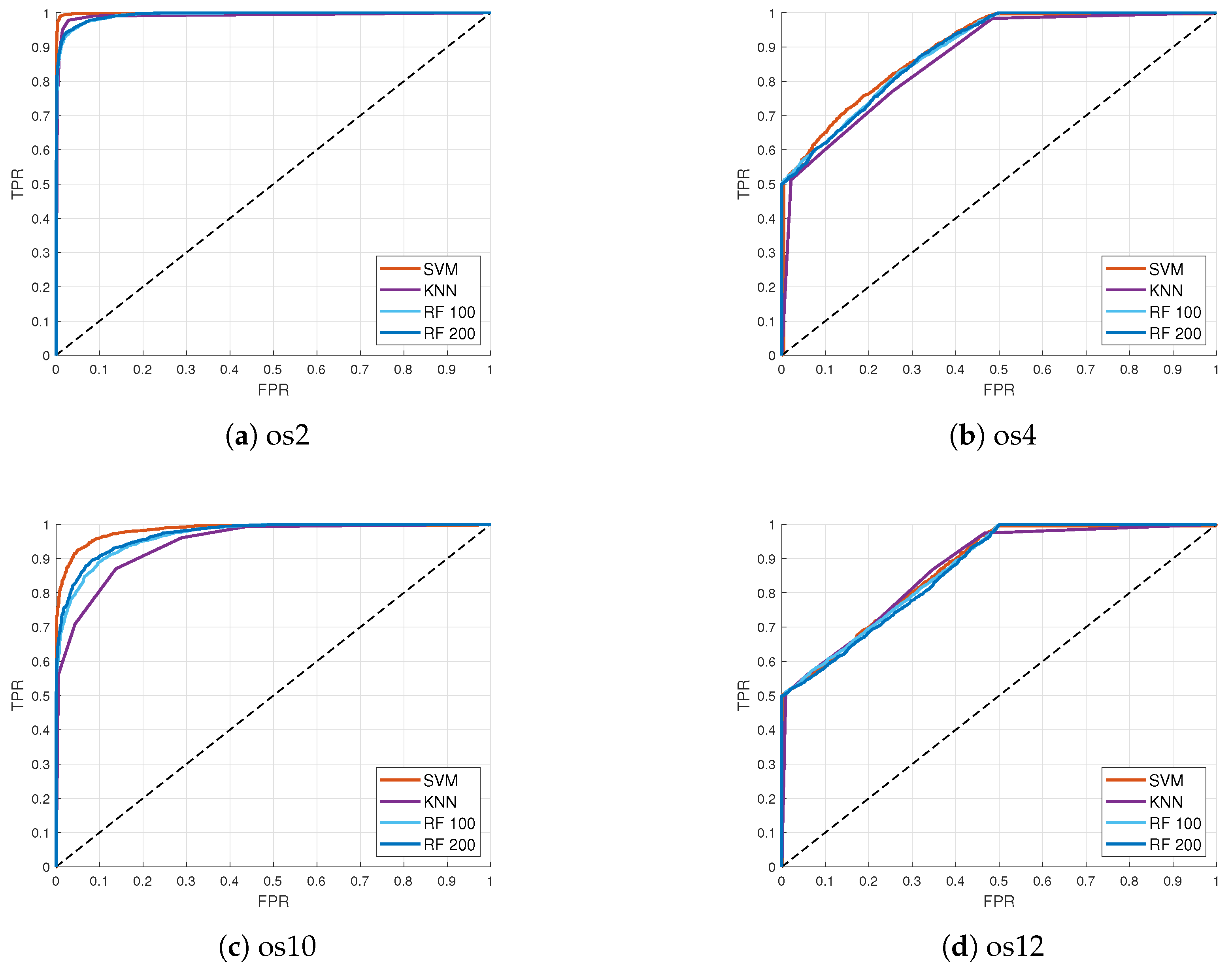
Figure 2 shows Receiver Operating Characteristic (ROC) curves for the signal-type classification based on images and db4 wavelet in the GPS and Galileo datasets. The x-axis represents false positive rate values while true positive rate values are represented on the y-axis. In Figure 2a,c, ROC curves have similar behavior for all ML models on the os2 and os10 datasets: SVM, KNN, RF-100, and RF-200. All models had high classification accuracy although the SVM model gave the highest accuracy in both cases. The classification results for the GPS os2 dataset were better compared to those of the Galileo os10 dataset. Similar results were obtained for datasets os4 and os12, as shown in Figure 2b,d. Although SVM stood out as the best model with the highest accuracy, ROC curves had significant distortion in their form because of lower classification accuracy in those datasets. Lower classification accuracy was achieved due to a small power level advantage of 0.4 dB between fake and authentic signals. The obtained classification results for these datasets were expected when considering the power level advantage of 10 dB for fake signals in relation to authentic signals in the os2 and os10 datasets.
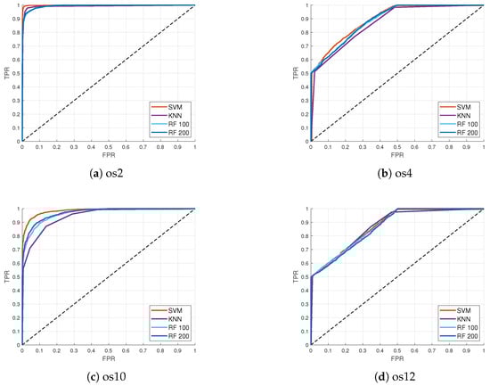
Figure 2.
ROC curves for different datasets and ML models for signal-type classification based on images using db4 wavelet in GPS (a) os2 (power level advantage 10 dB for fake signals), (b) os4 (power level advantage 0.4 dB for fake signals), and Galileo (c) os10 (power level advantage 10 dB for fake signals), (d) os12 (power level advantage 0.4 dB for fake signals) datasets.
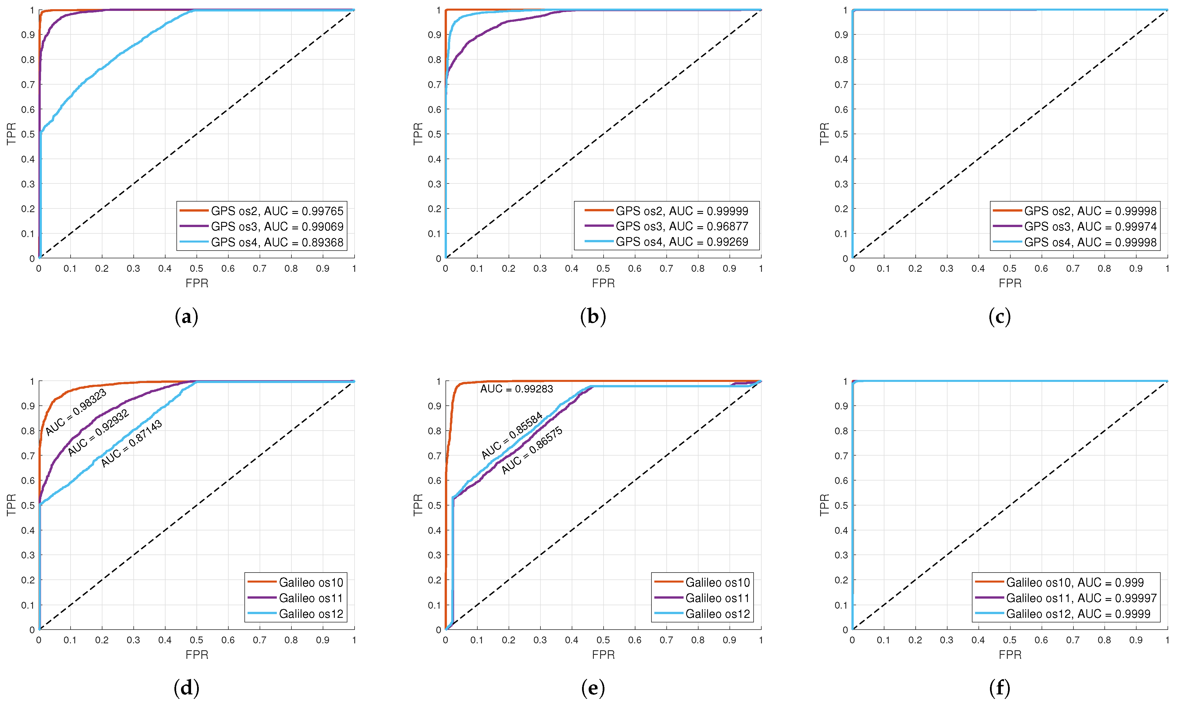
The ROC curves for the SVM classification on GPS and Galileo datasets based on different types of input data are shown in Figure 3. From the attached figures, it is evident that all the curves have quite good shapes, but the curves in Figure 3c,f stand out, because they have an almost perfect shape, which indicates a very high accuracy of classification and an Area Under Curve (AUC) value almost equal to one. The lowest classification accuracy was achieved when images for both GPS and Galileo were taken as the input data. In the case of images and image features as the input data, the results for Galileo were slightly worse compared to those for GPS. The reasons for this may be the more advanced modulation technique Binary Offset Carrier (BOC) used by Galileo, geographical coverage, and satellite geometry, because GPS has a wider and more stable coverage while Galileo is still under development and there may be a smaller number of visible satellites at any given time. Also, Galileo can have multiple errors in signal characteristics resulting in more difficult classification.
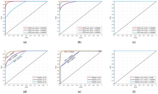
Figure 3.
ROC curves for SVM classification based on different types of input data for GPS datasets: (a) images, (b) images’ extracted features, (c) statistical and spectral features; and Galileo datasets: (d) images, (e) images’ extracted features, (f) statistical and spectral features.
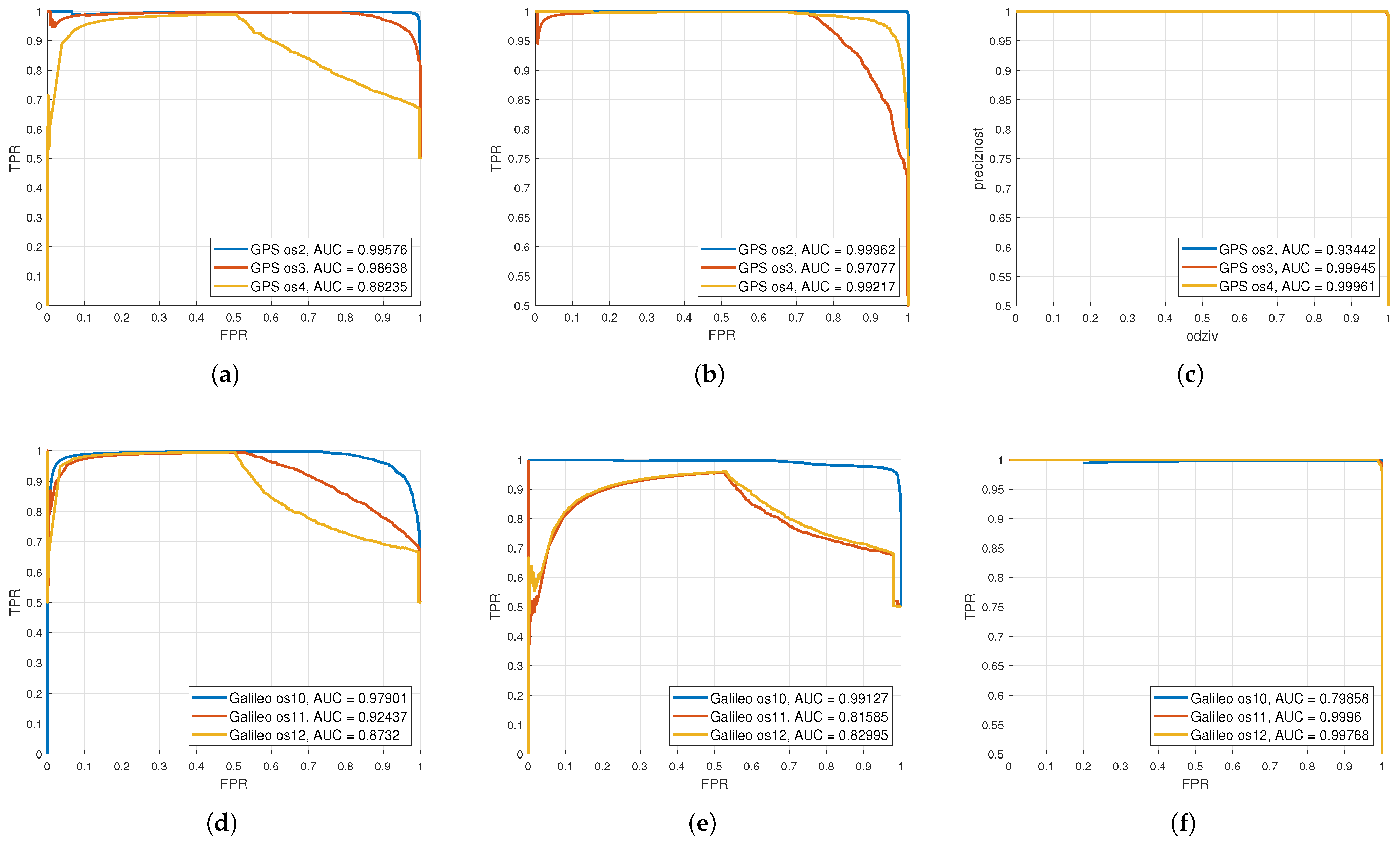
From Figure 4, it can be seen that statistical and spectral features as input data for the classification of SVM models had the highest accuracy and the values of R and P were almost equal to one, which is the ideal case. For example, for the case when the input was an image, the accuracy for os4 was 78.2%, recall was 0.7792, precision was 0.7867, and the PR curve was quite distorted. In the case when the input features were images, the accuracy for os12 was 76.43%, recall was 0.7712, precision was 0.7515, and the PR curve was quite distorted compared to GPS os4. Precision and recall values greater than 0.7 indicate a good classification model. Low precision (P < 0.5) means that the classifier has a large number of false positive samples that may be the result of an unbalanced class or unadjusted model hyperparameters. When the precision value is to close one, it means that the model has not missed any real positive results and is able to classify correct and incorrect sample labeling well. Low response (R < 0.5) means that the classifier has a large number of false negative samples that may be the result of an unbalanced class or unadjusted model hyperparameters. Ideally, R = 1, i.e., all positive samples are marked as positive by the classifier. It is ideal when all positively classified samples are really positive (P = 1) and, conversely, all positive samples are also classified as positive (R = 1).
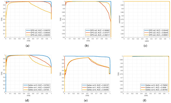
Figure 4.
Precision–recall curves for SVM classification on the GPS os2, os3, and os4 and Galileo os10, os11, and os12 datasets based on different types of input data: (a) image (GPS), (b) images’ extracted features (GPS), (c) statistical and spectral features (GPS), (d) image (Galileo), (e) images’ extracted features (Galileo), (f) statistical and spectral features (Galileo).
The performance parameters of the signal-type classification model for the different machine learning models for the db4 and db8 GPS wavelets and the different input classification data are shown in Table 2. The obtained classification values of several parameters for the SVM, KNN, RF-100, and RF-200 methods applied to the approximation coefficients based on the os2 and os4 datasets are presented. The performance parameters analyzed were the mean value of the model accuracy, F1-score, recall, and precision. Furthermore, a parameter that shows the time needed to run a particular model was added. From the table, we can see that, for example, the mean accuracy values were the same for both the db4 and db8 wavelets. As for the classification with images as input data, the highest accuracy for both types of wavelets (db4 and db8) was obtained by the SVM model on the os2 dataset, with values of 98.94% and 99.43%, respectively. It can be concluded that the SVM with Gaussian (RBF) kernel achieved the best performance results because it implicitly handled local variations in signal power, critical for spoofing detection with small dB advantages such as os4 and os12.
Table 2.
Performance metrics for ML signal-type classification for the GPS dataset with db4 and db8 wavelets calculated for different input data: (a) images (blue), (b) extracted image features (orange), (c) statistical and spectral features (green).
The results for both spectral and statistical image characteristics were all equally good, and the RF-100 and RF-200 models stood out for the statistical ones with an accuracy of 100% and F1, R, and P values that amounted to one. The only difference between the two models was in the runtime because RF-200 had more trees compared to RF-100, and it took longer to run. The number of trees was gradually increased and values above 200 trees did not give any significant accuracy improvements but only increased the execution time and computational complexity. Our model achieved stability with 100–200 trees, and adding more trees did not improve performance metrics. When OOB estimates and cross-validation results for the RFs were compared, cross-validation gave slightly better results than OOB in the case of weak spoofing attacks such as in the os4 and os12 datasets. For example, for the os4 dataset and an RF with 100 trees, the F1-score for OOB was around 0.7 while the F1-score for cross-validation had a value of 0.7742. For os2 and an RF with 100 trees, the F1-score for cross-validation was 0.9537 while for OOB, it was 0.91. The values of R and P were all greater than 0.7, which indicated good classification models. The runtime of models that had images as input was much higher compared to models that took numerical values as input. The maximum run time was 1202 s for the RF-200 model on the os2 dataset because that model was the most complex due to the number of trees.
The values of the model performance parameters obtained for the Galileo os10 and os12 datasets are shown in Table 3. With Galileo, slightly worse results were obtained for all parameters. The SVM stood out as the best model when images were used as input classification data. As already mentioned, the Galileo system gives worse results because of the more advanced modulation technique used, geographical coverage, and satellite geometry because GPS has a wider and more stable coverage, while Galileo is still under development and there may be a smaller number of visible satellites at any given time. Also, Galileo can have multiple errors in signal characteristics, resulting in more difficult classification.
Table 3.
Performance metrics for ML signal-type classification for the Galileo dataset using db4 and db8 wavelets calculated for different input data: (a) images (blue), (b) extracted image features (orange), (c) statistical and spectral features (green).
The results obtained for Galileo for all three cases (images, image features, and statistical characteristics) showed a significant difference in accuracy between the os10 and os12 datasets. This was not the case for the statistical characteristics of the db4 wavelet.
Computational Complexity
Table 4 shows the computational complexity for the code parts for the SVM model classification algorithm based on various classification inputs: images, features extracted from images, and spectral and statistical features. From the table, it can be seen that the algorithm based on images as the input data differs from the other two in two steps, which are the generation of bag of features in which the image processing models are used, and the step in which the features are extracted from each generated image using the Speeded-Up Robust Feature (SURF) method. In algorithms where the input data were image characteristics and spectral and statistical features, the input data to the model were a series, and therefore, the computational complexity for these algorithms was lower compared to that of algorithms using images as inputs. As for other machine learning models, KNN and RF, they differed from the SVM in the step of training and testing the model.
Table 4.
SVM classification algorithms [57,58,59] described in steps with the computational complexity based on different type of data processing.
The calculation of computational complexity in parts for the proposed DWT algorithm is shown below:
- Loading IQ data from .bin file: , where S is the total number of samples per iteration; , where D is the number of samples in the observed particle of the signal, and P is the number of particles into which the signal is divided per iteration.
- Conversion of a 1D complex signal to a square matrix (combination ) to a 2D matrix of dimensions nxn: .
- Single-use 2D DWT: .
- Extraction of statistical characteristics for the first level of approximation coefficients: .
- Extraction of spectral features and FFT: .
- Saving features to .csv file: .
- Generating and saving DWT image (A1img) in .tiff format: .
- Feature extraction from the .tiff image:
- Histogram per RGB channel: , where C is the number of channels of the image (three channels for RGB).
- Gradient magnitude: .
- Textural features: , where G is the number of GLCM metrics (e.g., contrast, correlation, energy, and homogeneity).
The total complexity per iteration is ). The dominant part of computational complexity is the application of the 2D DWT transform, followed by the application of the Fast Fourier Transform and the extraction of features from images. The computational complexity for the entire processing of .bin file is , where R is the total number of iterations. If P and D increase, then the complexity goes over which is very memory-intensive. The computational complexity increases with the use of a larger number of levels, i.e., multiple decomposition levels and for this reason, only one DWT level was used in this research, which enabled faster and simpler batch processing of .bin file.
Table 5 shows the computational complexity for all machine learning and discrete waveform classification models used, where N is the total number of samples/images in the dataset, D is the number of features detected per image (it does not use the entire pixel space, but features are taken at certain grid positions; it takes 70% of the most prominent features), K is the number of clusters in the bag-of-features model (the number of visual words), I represents the number of clustering iterations, R is the number of repetitions of k-fold cross-validation, k is the number of folds in K-fold cross-validation, M is the number of training samples per iteration, d is the dimension of the BoF vector (the number of features after encoding), T is the number of test samples, S is the number of support vectors, and is the number of trees in the RF model.
Table 5.
Computational complexity for ML methods based on different classification data.
The computational complexity of the SVM model that uses images as the input classification data consists of two parts. The first part refers to the generation of the bag of features, while the second part refers to the k-fold cross-validation. The most critical term can be highlighted as , which grows quadratically for the Gaussian kernel (it can go up to ). The computational complexity of this model can be reduced by reducing the image resolution, converting the image to gray scale, using a linear kernel instead of a Gaussian kernel, extracting features, reducing the number of validation iterations, and reducing the number of folds (for this reason, in this study, the number of iterations was equal to three and the number of folds was five). If we compare the algorithm that uses and processes images as the input data, i.e., that generates a BoF, and algorithms that use image features and statistical and spectral features, it can be concluded that the algorithm that uses the BoF approach is more complex because it includes the extraction of key features, clustering into visual words, and encoding each image into a word histogram. On the other hand, algorithms that use precomputed features are much easier to process (lower complexity, faster processing, and lower memory requirements) because there is no need for feature extraction, image decoding, or clustering.
In the KNN model, no explicit data training is performed, but the model stores all the training data, so the computational complexity for training is negligible and amounts to [60]. In the KNN model that has images as input data, the BoF approach is also the most complex step. KNN classification is simpler to implement but has quadratic complexity in terms of the number of data for prediction, which can be complex for large datasets.
BoF feature extraction and RF model training are the most dominant members of the computational complexity of an RF model that uses images as input data [46]. In the case of precomputed features, the dominant members are parsing the .csv files and training the model due to the number of trees. This algorithm is faster than RF with images because it does not use BoF. It is suitable for large datasets, and the complexity depends on the number of trees, the number of features, and the size of the dataset.
The highest computational complexity is that of KNN with images as input because it has a quadratic complexity in the number of samples , and in combination with BoF image processing, it represents the most complex approach. On the other hand, the lowest complexity is that of the SVM which uses pre-extracted features, because it does not have a quadratic complexity of nor any BoF processing, and if M is not too large, this is the simplest approach in terms of computational complexity.
5. Conclusions
This paper proposed an integrated approach which combined the discrete wavelet transform and machine learning for spoofing attack detection and signal-type classification in the pre-correlation phase. The paper aimed to investigate radio frequency fingerprinting methods with emphasis on the discrete wavelet transform, which is in its infancy in the GNSS field. The motivation for the research presented in this paper was to show how the DWT and machine learning methods could be used for the successful detection of spoofing attacks and signal-type classification. The motivation was also to try to reduce computational complexity by using some other data type than an image. For the first time, in this research, radio frequency fingerprinting methods were applied on OAKBAT’s static scenarios and different satellite constellations (GPS and Galileo).
Models performance metrics showed that all machine learning models achieved very good classification results, but generally, the SVM with a Gaussian kernel exhibited the best behavior for the different types of input data, both GPS and Galileo constellations, and both types of the used Daubechies wavelets, db4 and db8. For example, for images as the input data, the SVM for the GPS os2 dataset (where authentic signals have a 10 dB power advantage compared to fake signals) achieved 98.94% accuracy for the db4 and 99.43% for the db8 wavelet. On the other hand, the SVM method for the GPS os4 dataset in which authentic signals have a 0.4 dB power advantage to fake signals, had worse results with an accuracy of 78.20% for the db4 and 75.69% for the db8 wavelet. The same behavior of the models applied to the Galileo os10 and os12 datasets, which are equivalent to the GPS os2 and os4 datasets in terms of power level.
Generally, in comparison with GPS, Galileo had slightly worse results for all parameters. The reason was the geographical coverage and satellite geometry, because GPS has a wider and more stable coverage, while Galileo is still under development. When comparing the os2 with the os10 dataset for images as the input data and the SVM method for the db4 wavelet, os2 had an accuracy of 98.94% and os10 had an accuracy of 93.94%. The same was true when comparing os4 with os12. For images as the input data and SVM as the classification method, the accuracy for os4 was 78.20% and the accuracy for os12 was 75%. Regarding the wavelet type, the application of both db4 and db8 gave good results.
Regarding the computational complexity, the highest was for the KNN method which used images as input classification data due to the dominant quadratic complexity . The lowest computational complexity was obtained by the SVM method which used pre-extracted features for classification. It can be concluded that the input data type significantly affects the computational complexity and choosing pre-extracted features for classification reduces the computational complexity.
The evaluation results showed that the proposed integrated approach gave very good results in spoofing attack detection and signal-type classification. Based on the results in this paper, it can be concluded that the SVM model with a Gaussian kernel in combination with Daubechies db4 and db8 wavelets represents a robust and powerful approach in weak- and high-spoofing scenarios. Furthermore, it is the most suitable for use in terms of computational complexity and with the different types of input classification data. Using pre-extracted features as input classification data reduces the computational complexity.
To confirm the robustness of the proposed approach, future work will include the application of the integrated approach on different GPS and Galileo datasets by combining approximation and detail DWT coefficients and several decomposition levels. Furthermore, experiments with some other types of wavelets will be performed. Since in this research, synthetic spoofing attacks simulated in the “open-sky” environment were used, our plan is to include datasets with different propagation environments, which will allow more realistic testing of the proposed approach. This research confirms the reliability of our approach in case of intermediate spoofing attacks, and the plan for the future is to test the reliability of the proposed approach in complex sophisticated spoofing attacks.
Author Contributions
Article conceptualization, K.B. and M.B.; literature research and data processing, K.B. and M.B.; methodology, K.B. and M.B.; validation, K.B. and M.B.; investigation, K.B. and M.B.; writing—original draft preparation, K.B. and M.B.; writing—review and editing, K.B., M.B., and D.B.; visualization, K.B. and M.B.; supervision, D.B.; project management, D.B. All authors have read and agreed to the published version of the manuscript.
Funding
This research received no external funding.
Data Availability Statement
OAKBAT datasets were used in this research. The datasets are publicly available.
Conflicts of Interest
Author Marta Balić was employed by the company Ericsson Nikola Tesla and is a PhD student at the University of Split. The authors declare that the research was conducted in the absence of any commercial or financial relationships that could be construed as potential conflicts of interest.
Abbreviations
The following abbreviations are used in this manuscript:
| AUC | Area Under Curve |
| BOC | Binary Offset Carrier |
| BoF | Bag-of-Features |
| CNN | Convolutional Neural Networks |
| DoA | Direction of Arrival |
| DWT | Discrete Wavelet Transform |
| FFT | Fast Fourier Transform |
| FPR | False Positive Rate |
| GLCM | Gray Level Co-Occurrence Matrix |
| GNSS | Global Navigation Satellite System |
| GPS | Global Positioning System |
| I/Q | In-phase and Quadrature |
| KNN | k-Nearest Neighbors |
| ML | Machine Learning |
| NMEA | National Marine Electronics Association |
| NN | Neural Networks |
| OAKBAT | Oak Ridge Spoofing and Interference Test Battery |
| OOB | Out-of-Bag |
| PR | Precision Recall |
| RBF | Radial Basis Function |
| RF | Random Forest |
| RFF | Radio Frequency Fingerprinting |
| RGB | Red, Green, and Blue |
| ROC | Receiver Operating Characteristic |
| SDR | Software-Defined Radio |
| SQM | Signal Quality Monitoring |
| SURF | Speeded Up Robust Features) |
| SVM | Support Vector Machine |
| TEXBAT | Texas Spoofing Test Battery |
| ToA | Time of Arrival |
| TPR | True Positive Rate |
References
- Humphreys, T.E.; Ledvina, B.M.; Psiaki, M.L.; O’Hanlon, W.B.; Kintner, P.M. Assessing the Spoofing Threat: Development of a Portable GPS Civilian Spoofer. In Proceedings of the 21st International Technical Meeting of the Satellite Division of The Institute of Navigation (ION GNSS Conference), Savannah, GA, USA, 16–19 September 2008. [Google Scholar]
- Babić, K. Spoofing Signal Detection in Global Navigation Satellite System. Ph.D. Thesis, University of Split, Faculty of Electrical Engineering, Mechanical Engineering and Naval Architecture, Split, Croatia, 2025. [Google Scholar]
- Zhang, L.; Wang, L.; Wu, R.; Zhuang, X. A new approach for GNSS spoofing detection using power and signal quality monitoring. Meas. Sci. Technol. 2024, 35, 126109. [Google Scholar] [CrossRef]
- Lee, D.K.; Miralles, D.; Akos, D.; Konovaltsev, A.; Kurz, L.; Lo, S.; Nedelkov, F. Detection of GNSS Spoofing using NMEA Messages. In Proceedings of the European Navigation Conference (ENC), Dresden, Germany, 23–24 November 2020. [Google Scholar] [CrossRef]
- Truong, V.; Vervisch-Picois, A.; Rubio Hernan, J.; Samama, N. Characterization of the Ability of Low-Cost GNSS Receiver to Detect Spoofing Using Clock Bias. Sensors 2024, 23, 2735. [Google Scholar] [CrossRef] [PubMed]
- Yang, Q.; Chen, Y. A GPS Spoofing Detection Method Based on Compressed Sensing. In Proceedings of the IEEE International Conference on Signal Processing, Communications and Computing (ICSPCC), Xi’an, China, 25–27 October 2022. [Google Scholar] [CrossRef]
- Jafarnia-Jahromi, A.; Broumandan, A.; Nielsen, J.; Lachapelle, G. GPS vulnerability to spoofing threats and a review of antispoofing techniques. Int. J. Navig. Obs. 2012, 2012, 127072. [Google Scholar] [CrossRef]
- Lee, Y.S.; Yeom, J.S.; Jung, B.C. A Novel Array Antenna-Based GNSS Spoofing Detection and Mitigation Technique. In Proceedings of the IEEE 20th Consumer Communications & Networking Conference (CCNC), Las Vegas, NV, USA, 8–11 January 2023. [Google Scholar] [CrossRef]
- Li, J.; Li, W.; He, S.; Dai, Z.; Fu, Q. Research on Detection of Spoofing Signal with Small Delay Based on KNN. In Proceedings of the IEEE 3rd International Conference on Electronics Technology (ICET), Chengdu, China, 8–12 May 2020. [Google Scholar] [CrossRef]
- Yang, B.; Tian, M.; Ji, Y.; Cheng, J.; Xie, Z.; Shao, S. Research on GNSS Spoofing Mitigation Technology Based on Spoofing Correlation Peak Cancellation. IEEE Commun. Lett. 2022, 26, 3024–3028. [Google Scholar] [CrossRef]
- Meng, L.; Yang, L.; Yang, W.; Zhang, L. A Survey of GNSS Spoofing and Anti-Spoofing Technology. Remote Sens. 2022, 14, 4826. [Google Scholar] [CrossRef]
- Khoei, T.T.; Gasimova, A.; Ahajjam, M.A.; Shamaileh, K.A.; Devabhaktuni, V.; Kaabouch, N. A Comparative Analysis of Supervised and Unsupervised Models for Detecting GPS Spoofing Attack on UAVs. In Proceedings of the 2022 IEEE International Conference on Electro Information Technology (eIT), Minnesota State University, Mankato, MN, USA, 19–21 May 2022. [Google Scholar] [CrossRef]
- Shafique, A.; Mehmood, A.; Elhadef, M. Detecting Signal Spoofing Attack in UAVs Using Machine Learning Models. IEEE Access 2021, 9, 93803–93815. [Google Scholar] [CrossRef]
- Gallardo, F.; Yuste, A.P. SCER Spoofing Attacks on the Galileo Open Service and Machine Learning Techniques for End-User Protection. IEEE Access 2020, 8, 85515–85532. [Google Scholar] [CrossRef]
- Semanjski, S.; Semanjski, I.; De Wilde, W.; Muls, A. Use of Supervised Machine Learning for GNSS Signal Spoofing Detection with Validation on Real-World Meaconing and Spoofing Data—Part I. Sensors 2020, 20, 1171. [Google Scholar] [CrossRef]
- Chen, Z.; Li, J.; Li, J.; Zhu, X.; Li, C. GNSS Multiparameter Spoofing Detection Method Based on Support Vector Machine. IEEE Sens. J. 2022, 22, 17864–17874. [Google Scholar] [CrossRef]
- Elango, A.; Ujan, S.; Ruotsalainen, L. Disruptive GNSS Signal detection and classification at different Power levels Using Advanced Deep-Learning Approach. In Proceedings of the International Conference on Localization and GNSS (ICL-GNSS), Tampere, Finland, 7–9 June 2022. [Google Scholar] [CrossRef]
- Borhani-Darian, P.; Li, H.; Wu, P.; Pau, C. Detecting GNSS spoofing using deep learning. EURASIP J. Adv. Signal Process. 2024, 2024, 14. [Google Scholar] [CrossRef]
- Marchand, M.; Toumi, A.; Seco-Granados, G.; Lopez-Salcedo, J.A. Machine Learning Assessment of Anti-Spoofing Techniques for GNSS Receivers. In Proceedings of the WIPHAL 2023: Work-in-Progress in Hardware and Software for Location Computation, CEUR Workshop Proceedings, Castellon, Spain, 6–8 June 2023. [Google Scholar]
- Kuciapinski, K.S.; Temple, M.A.; Klein, R.W. ANOVA-based RF DNA analysis: Identifying significant parameters for device classification. In Proceedings of the International Conference on Wireless Information Networks and Systems (WINSYS), Athens, Greece, 26–28 July 2010. [Google Scholar]
- Danev, B.; Zanetti, D.; Capkun, S. On Physical-Layer Identification of Wireless Devices. ACM Comput. Surv. 2012, 45, 6. [Google Scholar] [CrossRef]
- Baldini, G.; Giuliani, R.; Steri, G.; Neisse, R. Physical layer authentication of Internet of Things wireless devices through permutation and dispersion entropy. In Proceedings of the Global Internet of Things Summit (GIoTS), Geneva, Switzerland, 6–9 June 2017. [Google Scholar]
- Baldini, G.; Gentile, C.; Giuliani, R.; Steri, G. Comparison of techniques for radiometric identification based on deep convolutional neural networks. Electron. Lett. 2019, 55, 62–114. [Google Scholar] [CrossRef]
- Fadul, M.K.M.; Reising, D.; Sartipi, M. Identification of OFDM-Based Radios Under Rayleigh Fading Using RF-DNA and Deep Learning. IEEE Access 2021, 9, 17100–17113. [Google Scholar] [CrossRef]
- Gahlawat, S. Investigation of RF Fingerprinting Approaches in GNSS. Ph.D. Thesis, Tampere University, Tampere, Finland, 2020. [Google Scholar]
- Wang, W.; Aguilar Sanchez, I.; Caparra, G.; McKeown, A.; Whitworth, T.; Lohan, E. A Survey of Spoofer Detection Techniques via Radio Frequency Fingerprinting with Focus on the GNSS Pre-Correlation Sampled Data. Sensors 2021, 21, 3012. [Google Scholar] [CrossRef]
- Morales-Ferre, R.; Wang, W.; Sanz-Abia, A.; Lohan, E.S. Identifying GNSS Signals Based on Their Radio Frequency (RF) Features—A Dataset with GNSS Raw Signals Based on Roof Antennas and Spectracom Generator. Data 2020, 5, 18. [Google Scholar] [CrossRef]
- Wang, W.; Lohan, E.S.; Sanchez, I.A.; Caparra, G. Pre-correlation and post-correlation RF fingerprinting methods for GNSS spoofer identification with real-field measurement data. In Proceedings of the 10th Workshop on Satellite Navigation Technology (NAVITEC), Noordwijk, The Netherlands, 4–8 April 2022. [Google Scholar] [CrossRef]
- Radoš, K.; Brkić, M.; Begušić, D. GNSS Signal Classification based on Machine Learning Methods. In Proceedings of the 47th MIPRO ICT and Electronics Convention (MIPRO), Opatija, Croatia, 20–24 May 2024. [Google Scholar] [CrossRef]
- Li, J.; Wu, H.; Gao, J.; Liu, F.; Zhang, Y.; Li, G. Performance Testing and Analysis of a New GNSS Spoofing Detection Method in Different Spoofing Scenarios. IEEE Access 2025, 13, 54779–54793. [Google Scholar] [CrossRef]
- Zhang, X.; Huang, Y.; Tian, Y.; Lin, M.; An, J. Noise-Like Features Assisted GNSS Spoofing Detection Based on Convolutional Autoencoder. IEEE Sens. J. 2023, 23, 25473–25486. [Google Scholar] [CrossRef]
- Humphreys, T.E.; Bhatti, J.A.; Shepard, D.P.; Wesson, K.D. The Texas Spoofing Test Battery: Toward a Standard for Evaluating GPS Signal Authentication Techniques. In Proceedings of the 25th International Technical Meeting of the Satellite Division of The Institute of Navigation, Nashville, TN, USA, 17–21 September 2012. [Google Scholar]
- Manfredini, E.; Dovis, F.; Motella, B. Validation of a signal quality monitoring technique over a set of spoofed scenarios. In Proceedings of the Proceedings of the 7th ESA Workshop on Satellite Navigation Technologies and European Workshop on GNSS Signals and Signal Processing (NAVITEC), Noordwijk, The Netherlands, 3–5 December 2014. [Google Scholar] [CrossRef]
- Chengjun, G.; Zhongpei, Y. Robust RF Fingerprint Extraction Scheme for GNSS Spoofing Detection. In Proceedings of the 36th International Technical Meeting of the Satellite Division of The Institute of Navigation (ION GNSS+ 2023), Denver, CO, USA, 11–15 September 2023. [Google Scholar] [CrossRef]
- Mehr, I.; Dovis, F. A deep neural network approach for classification of GNSS interference and jammer. IEEE Trans. Aerosp. Electron. Syst. 2024, 61, 1660–1676. [Google Scholar] [CrossRef]
- Albright, A.; Powers, S.; Bonior, J.; Combs, F. Oak Ridge Spoofing and Interference Test Battery (OAKBAT); Oak Ridge National Lab. (ORNL): Oak Ridge, TN, USA, 2020. [CrossRef]
- Mallat, S. Wavelet Tour of Signal Processing; Academic Press: Cambridge, MA, USA, 2008. [Google Scholar]
- Daubechies, I. Ten Lectures on Wavelets; SIAM: Philadelphia, PA, USA, 1992. [Google Scholar]
- Strang, G.; Nguyen, T. Wavelets and Filter Banks; Wellesley-Cambridge Press: Wellesley, MA, USA, 1996. [Google Scholar]
- Cortes, C.; Vapnik, V. Support-vector networks. Mach. Learn. 1995, 20, 273–297. [Google Scholar] [CrossRef]
- Fix, E.; Hodges, J.L. Discriminatory Analysis. Nonparametric Discrimination: Consistency Properties. Int. Stat. Rev./Rev. Int. De Stat. 1989, 57, 238–247. [Google Scholar] [CrossRef]
- Cover, T.; Hart, P. Nearest Neighbor Pattern Classification. IEEE Trans. Inf. Theory 1967, 13, 21–27. [Google Scholar] [CrossRef]
- Čulić Gambiroža, J. Machine Learning Methods for Efficient Data Reduction and Reconstruction in the concept of Internet of Things. Ph.D. Thesis, University of Split, Faculty of Electrical Engineering, Mechanical Engineering and Naval Architecture, Split, Croatia, 2023. [Google Scholar]
- Ho, T.K. The Random Subspace Method for Constructing Decision Forests. IEEE Trans. Pattern Anal. Mach. Intell. 1998, 20, 832–844. [Google Scholar] [CrossRef]
- Breiman, L.; Friedman, J.H.; Olshen, R.A.; Stone, C.J. Classification and Regression Trees; Routledge: Abingdon, UK, 2017. [Google Scholar]
- Breiman, L. Random Forests. Mach. Learn. 2001, 45, 5–32. [Google Scholar] [CrossRef]
- Šnajder, J. Machine Learning 1, 21. Model Evaluation; University of Zagreb, Faculty of electrical engineering and computing: Zagreb, Croatia, 2023. [Google Scholar]
- Joanes, D.N.; Gill, C.A. Comparing Measures of Sample Skewness and Kurtosis. J. R. Stat. Soc. Ser. D 1998, 47, 183–189. [Google Scholar] [CrossRef]
- Giannakopoulos, T.; Pikrakis, A. Audio Features. In Introduction to Audio Analysis: A MATLAB Approach; Elsevier: Amsterdam, The Netherlands, 2014; pp. 59–103. [Google Scholar] [CrossRef]
- Pilanci, M. EE269 Signal Processing for Machine Learning—Lecture 3 Part II: Spectral Features. 2021. Available online: https://web.stanford.edu/class/ee269/Lecture3_spectral_features.pdf (accessed on 22 February 2025).
- Kulkarni, N. Use of complexity based features in diagnosis of mild Alzheimer disease using EEG signals. Int. J. Inf. Technol. 2018, 10, 59–64. [Google Scholar] [CrossRef]
- Gonzalez, R.C.; Woods, R.E. Digital Image Processing, 3rd ed.; Pearson Prentice Hall: Upper Saddle River, NJ, USA, 2008. [Google Scholar]
- Pratt, W.K. Digital Image Processing: PIKS Scientific Inside, 4th ed.; Wiley-Interscience: Hoboken, NJ, USA, 2007. [Google Scholar]
- Bovik, A.C. (Ed.) Handbook of Image and Video Processing; Academic Press: San Diego, CA, USA, 2000. [Google Scholar]
- Haralick, R.M.; Shanmugam, K.; Dinstein, I. Textural Features for Image Classification. IEEE Trans. Syst. Man Cybern. 1973, SMC-3, 610–621. [Google Scholar] [CrossRef]
- Hall-Beyer, M. GLCM Texture: A Tutorial v. 3.0. 2017. Available online: https://prism.ucalgary.ca/handle/1880/51900 (accessed on 15 March 2025).
- Shalev-Shwartz, S.; Ben-David, S. Support Vector Machines. In Understanding Machine Learning: From Theory to Algorithms; Cambridge University Press: Cambridge, UK, 2014; Chapter 15; pp. 315–340. [Google Scholar]
- Bottou, L.; Lin, C.J. Support Vector Machine Solvers. In Large Scale Kernel Machines; Bottou, L., Chapelle, O., DeCoste, D., Weston, J., Eds.; MIT Press: Cambridge, MA, USA, 2007; pp. 301–320. [Google Scholar]
- Schölkopf, B.; Smola, A.J. Learning with Kernels: Support Vector Machines, Regularization, Optimization, and Beyond; Adaptive Computation and Machine Learning; MIT Press: Cambridge, MA, USA, 2002. [Google Scholar]
- Duda, R.O.; Hart, P.E.; Stork, D.G. Pattern Classification, 2nd ed.; Wiley-Interscience: New York, NY, USA, 2001. [Google Scholar]
Disclaimer/Publisher’s Note: The statements, opinions and data contained in all publications are solely those of the individual author(s) and contributor(s) and not of MDPI and/or the editor(s). MDPI and/or the editor(s) disclaim responsibility for any injury to people or property resulting from any ideas, methods, instructions or products referred to in the content. |
© 2025 by the authors. Licensee MDPI, Basel, Switzerland. This article is an open access article distributed under the terms and conditions of the Creative Commons Attribution (CC BY) license (https://creativecommons.org/licenses/by/4.0/).