Article

Calculating the Singular Values of Many Small Matrices on GPUs

Dipartimento di Ingegneria Elettrica e delle Tecnologie dell’Informazione, Università di Napoli Federico II, via Claudio 21, I 80125 Napoli, Italy
*
Author to whom correspondence should be addressed.
Electronics 2025, 14(16), 3217; https://doi.org/10.3390/electronics14163217
Submission received: 6 May 2025 / Revised: 9 August 2025 / Accepted: 11 August 2025 / Published: 13 August 2025

Abstract

This paper presents a fast and robust approach to evaluate the singular values of small (e.g., 4 × 4 , 5 × 5 ) matrices on single- and multi-Graphics Processing Unit (GPU) systems, enabling the modulation of the accuracy–speed trade-off. Targeting applications that require only computations of the SVs in electromagnetics (e.g., Multiple Input Multiple Output—MIMO link capacity optimization) and emerging deep-learning kernels, our method contrasts with existing GPU singular value decomposition (SVD) routines by computing singular values only, thereby reducing overhead compared to full-SVD libraries such as cuSOLVER’s gesvd and MKL’s desvg. The method uses four steps: interlaced storage of the matrices in GPU global memory, bidiagonalization via Householder transformations, symmetric tridiagonalization, and root finding by bisection using Sturm sequences. We implemented the algorithm in CUDA and evaluated it on different single- and multi-GPU systems. The approach is particularly suited for the analysis and design of multiple-input/multiple-output (MIMO) communication links, where thousands of tiny SVDs must be computed rapidly. As an example of the satisfactory performance of our approach, the speed-up reached for large matrix batches against cuSOLVER’s gesvd has been around 20 for 4 × 4 matrices. Furthermore, near-linear scaling across multi-GPUs systems has been reached, while maintaining root mean square errors below 2.3 × 10 7 in single precision and below 2.3 × 10 13 in double precision. Tightening the tolerance from δ = 10 7 to δ = 10 9 increased the total runtime by only about 10%.

1. Introduction

One of the most useful result of linear algebra is the singular value decomposition (SVD), which is widely employed in many areas of applied research like inverse problems [1], data compression [2,3], and machine learning [4,5]. In electromagnetics, it has been fruitfully used in, among other topics, near-field antenna sampling [6], imaging [7,8], and optimization of multiple-input/multiple-output (MIMO) systems [9].

1.1. Application Context

In some of the applications, the full SVD computation, namely singular vectors and singular values (SVs), is required, while in others only SVs are necessary. For example, MIMO is a wireless communication technology that uses multiple antennas working in both transmission and reception modalities to increase the channel capacity over that of a conventional single-input/single-output (SISO) system. In this case, the channel capacity is a crucial parameter to evaluate the performance of a communication system, and the problem arises of how to define the most convenient antenna configuration to maximize it, given the signal-to-noise ratio and the propagation environment. The channel capacity is related to the SVs of the channel matrix, its optimization requires repeated calculation of the SVs [9], and so accelerating their computation is crucial even in the case of classically sized (i.e., 4 × 4 , 5 × 5 ) MIMO [10]. Of course, when only the SVs are required, calculating the SVs alone instead of the full SVD turns out to be more convenient, this problem being computationally less burdened.
Other applications requiring the computation of large batches of tiny matrices are astrophysics [11] and deep learning [12,13]. For example, in an astrophysical ordinary differential equation (ODE) solver, multiple subregions of the domain of interest are simulated, and each subregion corresponds to a small linear system to be analyzed. In the framework of deep learning, the singular values of the network layers are computed [12] in order to be, for example, bounded [13] to prevent the effect of ill-conditioning during training. Speaking more generally, a recent trend is occurring in redefining linear algebra algorithms for batches of small matrices [14]. For example, it has been shown that randomly sampling a matrix can lead to satisfactory approximations of its first singular values [15].
Performing an accurate and fast computation of SVs is a sensitive issue, especially when the calculation is part of a very large number of iterations, as in optimization problems [6,7,8,9]. In fact, in addition to the repeated evaluation, each iteration can require the computation of the SVs of many different matrices, either for global or local optimizations. Graphics Processing Units (GPUs) are a candidate computing platform to accelerate this task [16,17,18].

1.2. Limitations of Literature

The computation of singular values only on conventional computational platforms has been extensively explored in the literature [19]. Modern approaches to this problem have been presented in [20], where the QR method for upper-triangular semiseparable matrices has been applied after the original matrix has been reduced to bidiagonal form, and in [21], where a deep neural network-based approach has been proposed. Unfortunately, the problem dealt with in this paper has received little attention, since the approaches available for GPU processing have mainly focused on the computation of the full SVD of large batches of large matrices. The few GPU algorithms dealing with large batches of small/medium-sized matrices have tackled the problem of the full or reduced SVD calculation involving the computation of both singular values and singular vectors, and not the singular values only. For example, in [22], a W-cycle Jacobi SVD on an NVIDIA V100 running 4.5 faster than cuSOLVER has been proposed for the SVD computation of small/moderate matrix sizes (e.g., 32 × 32 , 48 × 48 ). In [23], a throughput exceeding 800 G F L O P / s in single-precision arithmetic using register/shared-memory optimizations has been achieved on K40/P100 systems for the SVD calculation of medium-sized matrices (e.g., 512 × 512 ). Finally, in [14], batched linear algebra solutions, including SVD, were investigated for matrices from small/moderate to medium sizes (up to 512 × 512 ).

1.3. Our Contributions

In this paper, we develop a fast and robust approach to evaluate the SVs of small (e.g., 4 × 4 , 5 × 5 ) matrices on GPUs capable of modulating the accuracy-speed trade-off. The primary requirement is developing GPU routines having a convenient computational cost so as to be faster than state-of-the-art libraries running on GPUs.
Obviously, the achievable effectiveness and efficiency of the approach are related to the features of the involved matrices that can be exploited as a priori knowledge and to the capability of taking advantage of the underlying architecture of the GPU at its best. Concerning the former point, many of the algebraic properties that lead to benefits in the computation of the SVs of large matrices, e.g., symmetry [24] or rotational symmetry [25], have little effect in the case of small matrices. Accordingly, and also to keep the approach general, in this paper we will exploit no such properties. Regarding the latter point, for the problem here considered and to gain the required effectiveness and efficiency, the computational scheme must be properly devised to exploit at best the Single Instruction Multiple Data (SIMD) paradigm of GPUs. We note that, although many schemes for the SV calculation have been developed, choosing and implementing the best approach matching the SIMD pattern is by no means an easy task when a large number of small matrices is involved. Here, for the very first time, we present an approach for the calculation of the SVs of many small matrices based on four steps that have been properly selected to match the SIMD architecture of a GPU:
  • Interlaced storage of the matrices in GPU global memory;
  • Bidiagonalization using Householder matrices [26];
  • Symmetric tridiagonalization of the bidiagonal matrix;
  • Root finding by bisection using Sturm sequences [27].
In summary, the contributions of this paper are threefold:
  • we introduce a novel, multi-GPU algorithm for computing the singular values of many small matrices via interlaced global memory storage, Householder-based bidiagonalization, tridiagonalization, and Sturm-sequence bisection, allowing direct control of the accuracy–speed trade-off via the tolerance parameter δ ;
  • we provide a CUDA implementation that achieves remarkable speedups over other existing approaches and whose target accuracy can be set to match MATLAB’s state-of-the-art svd routine;
  • we demonstrate the algorithm scalability across multiple GPUs and show the computational performance behavior against the target accuracy.
The implementation has been devised as follows.
First, a proper interlaced storage of the data matrices has been set up to guarantee coalesced memory accesses. This has been a key point of implementation, as the algorithm is memory bound. Second, it should be noted that the bidiagonalization step is not easy to parallelize and that the matrices involved are small, which makes thread cooperation not convenient for this task. Accordingly, in the proposed computational scheme, each GPU thread is in charge of calculating the whole bidiagonalization for a different matrix. We stress that this choice is strictly related to the size of the relevant matrices and that, conversely, for large matrices such a strategy would lead to unsatisfactory results. Third, since the approach based on Sturm sequences turns root finding into an embarrassingly parallel task, each different matrix eigenvalue is carried out in parallel by a different GPU thread, so that different GPU threads can compute eigenvalues of the same matrix in parallel.

1.4. Differences with the Literature

Targeting applications requesting the calculation of the SVs only, compared to the approaches in [14,22,23], our computational scheme calculates singular values alone, without the singular vectors, which eases the burden and enables much higher speedups against standard library routines compared to [14,22,23]. Furthermore, as will be shown, by a tunable tolerance, our approach is capable of reaching the same singular value computational accuracy of MKL or MATLAB, while the precision issue has been neglected in [22], can remain undefined in [23] in the cases of lack of convergence, is implicitly inherited by LAPACK’s Householder kernels, and is not directly controlled in [14].
It should also be noticed that, in recent years, the availability of multi-GPU systems, single nodes or multi-node, has spread [28]. In order to take into account such an availability, another key point of the developed approach has been exploiting part or all of the GPUs of the computing system by subdividing the batch of matrices for which the SVs are computed across the different underlying devices.
We finally want to stress that, to the best of our knowledge, the approach proposed for the multi-GPU calculation of the SVs of a large number of small matrices is an absolute novelty. Among others [14,23], one of the operational GPU routines available for the calculation of SVs of matrix batches is gesvd of the cuSOLVER library [29]. Nevertheless, as we shall see, the performance of such a routine is worse than the proposed computational scheme. Furthermore, throughout the literature, attention has been almost exclusively paid to GPU computations of the SVD for large matrices [30,31].
The algorithm has been implemented in the CUDA language and tested on several single- and multi-GPU systems.
The original, preliminary approach in [10] has been thoroughly optimized. Also, at variance with [10], the performance has been investigated over different single- and multi-GPU architectures, also in comparison to other GPU-based SV calculation routines.

1.5. Paper Layout

The paper is organized as in Figure 1. In Section 2, the most common methods to compute the SV are discussed, and the proposed approach is presented. In Section 3, the strategy adopted to implement the algorithm on the GPU is described. Section 4 shows the numerical results. Finally, in Section 5, conclusions are drawn and future developments are foreseen. A detailed description of the bidiagonalization (Algorithm 1) is given as well as CUDA-like snippets for the memory reorganization (Algorithm 2), bidiagonalization (Algorithm 3), bisection (Algorithm 4) and routines used in the root finding step (Algorithms A1 and A2) are reported. A list of all abbreviations used throughout the manuscript is finally provided in the Appendix A.

2. The Approach

2.1. Statement of the Problem

In the following, we will deal with the particular case of real matrices, the extension to complex matrices being a matter of a future activity. Furthermore, we will use the same MATLAB-like notation of [26] for vectors, matrices, and operations among them, which can now be considered as a standard in linear algebra applications. Finally, with no loss of generality, we will consider matrices A R m x n , with m n . Obviously, in the case m > n , it will be sufficient to compute the singular values of A T , the superscript T denoting transposition, since they coincide with those of A.
The problem of computing the singular values of a matrix can be theoretically reduced to that of finding the eigenvalues of a symmetric matrix. Indeed, the singular values of A are the square roots of the eigenvalues of the matrix A T A , or, equivalently, A A T . Likewise, the left (or right) singular vectors of A are equal to the eigenvectors of A A T  (or A T A ).

2.2. Literature Review

Much literature is available for the full computation (i.e., both singular values and singular vectors) of the SVD of a matrix. The two most popular techniques are
  • the Golub-Reinsch algorithm [26,32];
  • the one-sided Jacobi algorithm [33,34].
Other techniques include the bisection [27] and the divide and conquer [35] approaches.

2.2.1. The Golub-Reinsch Algorithm

The Golub–Reinsch algorithm is the standard for the computation of the SVD, and it is also used in the LAPACK package [26,32]. In particular, the Golub–Reinsch algorithm is a two-step one. The input matrix is first reduced to a bidiagonal matrix using a series of Householder transformations and then the bidiagonal matrix is diagonalized by performing implicit QR iterations.

2.2.2. The One-Sided Jacobi Method

The one-sided Jacobi method, instead, makes use of a sequence of pair-wise column orthogonalizations such that the input matrix is replaced, after a proper number of iterations, with a sufficiently orthogonal matrix according to a given tolerance [26,32].

2.2.3. Differences Between the Golub-Reinsch Algorithm and the One-Sided Jacobi Method

The Golub-Reinsch method appears to be more difficult to be parallelized, and its sequential version is faster than Jacobi-based algorithms on sequential machines [36,37]. On the other hand, the Jacobi method exhibits some degree of parallelism [38,39,40] and proves a better relative accuracy [41]. However, neither of the two methods cited above appears to be amenable to a meaningful parallel implementation with tiny (e.g., 4 × 4 , 5 × 5 ) matrices. Furthermore, we are here interested in the calculation of the SVs only, while the two above approaches aim at the full SVD computation.

2.2.4. Outline of Our Approach

As mentioned in the Introduction, the proposed approach to face the problem of computing the SVs of many small matrices is a three-step one. In Figure 2, we outline the four major stages of our algorithm:
  • Interlaced memory storage. A pre-processing step amounts to interlace the different matrices to be processed in order to enable coalesced memory accesses.
  • Bidiagonalization. The first step consists of reducing the input matrix into a bidiagonal form, following the same lines as the Golub-Reinsch algorithm.
  • Tridiagonalization. The second step performs a symmetric tridiagonalization of the bidiagonal matrix.
  • Root finding. The third step searches for the roots of the characteristic polynomial associated with the symmetric tridiagonal matrix by bisection using Sturm sequences.
In the following sections, we will briefly recall only the main mathematical principles behind the approach necessary to describe the implementation.
Figure 2. Block diagram of the proposed approach.
Electronics 14 03217 g002

2.3. First Step: Bidiagonalization

In this step, the generic real matrix A R m x n is bidiagonalized, namely, it is decomposed as
A = P B Q T ,
where B R m x n is an upper bidiagonal matrix and P R m x m and Q R n x n are orthogonal Householder matrices. The bidiagonalization is achieved by applying a series of Householder transformations to the matrix A with the aim of zeroing the elements below the diagonal along with the elements above the first superdiagonal. The bidiagonalization algorithm that we have employed and that we are now going to briefly recall is that presented by Golub and Van Loan in [26]. It is an iterative algorithm having a finite number of iterations. In particular, the number of iterations is n 1 if m = n ; otherwise, the number of iterations is n.

2.3.1. Householder Reflection

Before describing the bidiagonalization algorithm, we recall that a possible Householder vector h to eliminate entries below the top entry, namely, to make a given vector x R k x 1 proportional to a vector e R k x 1 = ( 1 , 0 , , 0 ) T is given by [26]
h = x + α e ,
where α = ± x . According to Equation (2) and on defining β = 2 / ( h T h ) and I k as the identity matrix of dimensions k × k , then [26]
( I k β h h T ) x = α e .
The vector h is also known as a reflector. A stable way to compute the Householder reflectors is described in [26] (see Algorithm 5.1.1, p. 210).
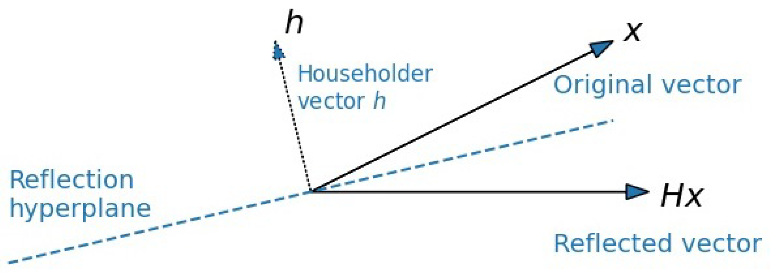
We can think of bidiagonalization as alternately “zeroing-out” columns and rows with simple reflection operations. Each reflector acts like placing a mirror at an angle to “bounce” a column (or row) so that all but its first entry vanish (Figure 3).

2.3.2. Iterations

The first operation of iteration #1 consists of selecting a left Householder vector u ( 1 ) of length m to zero the elements of A below the first element of the first column. The vector x is represented in this case by A ( 1 : m , 1 ) . Using u ( 1 ) as a reflector, we define the matrix A 1 as [26]
A 1 = ( I m β u ( 1 ) u ( 1 ) u ( 1 ) T ) A = X X X X 0 X X X 0 X X X X X X 0 X X X .
The second operation consists of defining a new matrix of size m × ( n 1 ) as A 1 = A 1 ( 1 : m , 2 : n ) , selecting a right Householder vector v ( 1 ) of length n 1 to zero the elements of A 1 to the right of the first element of the first row. In this case, the vector x is represented by A 1 ( 1 , 1 : n 1 ) . It should be noticed that a further requirement is that the Householder vectors be normalized such as v ( 1 ) ( 1 ) = 1 . Using v ( 1 ) as a reflector, we define the matrix A 2 as [26]
A 2 = A 1 ( I n 1 β v ( 1 ) v ( 1 ) v ( 1 ) T ) = x x 0 0 0 x x x 0 x x x x x x 0 x x x
where β u ( 1 ) = 2 / ( u ( 1 ) T u ( 1 ) ) , β v ( 1 ) = 2 / ( v ( 1 ) T v ( 1 ) ) and I is the identity matrix. In this way, A 2 shows zeros below the diagonal in the first column and to the right of the superdiagonal element of the first row, as requested.
The algorithm then proceeds in an analogous way with the annihilation of the second column A ( 2 : m , 2 ) and row A ( 2 , 3 : n ) and so on. If m > n , there are n columns and n 2 rows to eliminate. At the end of this process, an upper bidiagonal matrix B is obtained such that [26]
P = i = 1 n P i and Q = i = 1 n 2 Q i
with
P i = ( I β u ( i ) u ( i ) u ( i ) T ) and Q i = ( I β v ( i ) v ( i ) v ( i ) T ) .
The left Householder vectors u ( i ) ’s are vectors of length m with i 1 leading zeros, while the right Householder vectors v ( i ) ’s are vectors of length n with i leading zeros. They are needed to zero the elements of the ith column below the diagonal as well as to zero the elements of the ith row to the right of the superdiagonal element, respectively. Moreover, both left and right Householder vectors are normalized such that u ( i ) ( i ) = 1 and v ( i ) ( i + 1 ) = 1 .
From the computational standpoint, each left or right update of the bidiagonalization process consists of a Matrix-Vector Multiplication (MVM) and a rank-one update. Indeed, looking at the left matrix update at the ith step, the involved algebraic operations can be arranged as
( I β u ( i ) u ( i ) u ( i ) T ) A i = A i β u ( i ) u ( i ) y ( i ) T M V M R a n k - o n e   u p d a t e
where y ( i ) T R 1 x n = u ( i ) T A i is the relevant MVM and β u ( i ) u ( i ) y ( i ) T is the rank-one matrix involved in the update. The same holds true for the right matrix updates. Accordingly, each bidiagonalization step costs two MVMs and two rank-one updates. Actually, the ith bidiagonalization step can be written as
A i + 1 = ( I β u ( i ) u ( i ) u ( i ) T ) A i ( I β v ( i ) v ( i ) v ( i ) T ) .
It should be noticed that the operations in Equation (9) must be executed in a prescribed order since the ith right Householder vector v ( i ) is known only after the ith column has been annihilated. In other words, v ( i ) can be computed only after the ith row of ( I β u ( i ) u ( i ) u ( i ) T ) A i has been calculated. Nevertheless, let us ignore this issue for a while. With a little algebra, Equation (9) can be recast as
A i + 1 = A i u ( i ) z ( i ) w ( i ) MVM v ( i ) T R a n k - t w o   u p d a t e
where
w ( i )   =   β v ( i ) A i v ( i ) ,
x ( i )   =   β u ( i ) A i T u ( i ) ,
z ( i )   =   x ( i ) T M V M β v ( i ) ( x ( i ) T v ( i ) ) v ( i ) T .
Assuming we perform an in-place update of the input matrix, Equations (10)–(13) allow the set up of the bidiagonalization step as two MVMs and a single rank-two update, where u ( i ) z ( i ) w ( i ) v ( i ) T is the rank-two matrix involved in such an update. In other words, the mentioned equations enable deferring one of the two left rank-one matrix updates and saving a read-write operation as compared to the scheme in Equation (8). Concerning now the problem of knowing v ( i ) in advance, this issue can be solved by updating at least the ith row of the matrix A i prior to applying Equations (10)–(13). The described bidiagonalization approach is summarized in Algorithm 1.
Algorithm 1 Bidiagonalization.
if  m = = n   then
    n u m i t e r = n 1 ;
else
    n u m i t e r = n ;
end
for  i = 1 : n 2   do
 1. Compute the ith left Householder vector u ( i ) relative to the column A i ( i : m , i ) .
 2. Update the ith row of A i to compute v ( i ) = A i ( i , i + 1 : n ) β u ( i ) u ( i ) T A i ( i : m , i + 1 : n ) .
 3. Compute the ith right Householder vector v ( i ) from v ^ ( i ) .
 4. Compute w ( i ) and x ( i ) from (11) and (12), respectively.
 5. Compute z ( i ) from (13).
 6. Update the matrix A i using (10).
end
for  i = n 2 : n u m i t e r   do
 1. Compute the ith left Householder vector u ( i ) relative to the column A i ( i : m , i ) .
 2. Update the input matrix using (8):
   A i + 1 = ( I β u ( i ) u ( i ) u ( i ) T ) A i = A i β u ( i ) u ( i ) y ( i ) T .
end

2.4. Second Step: Tridiagonalization

Once the input matrix A has been transformed into a bidiagonal form B, then the singular values of A could be obtained by applying an implicit-shift QR algorithm to the symmetric tridiagonal matrix T = B T B .
It is known that, for numerical reasons, the explicit formation of the matrix T should be avoided since, depending on the nature and on the algebraic properties of B, the explicit computation of T could result in unnecessary loss of accuracy, especially in the calculation of the smallest singular values [27,32]. To avoid this problem, the Golub-Reinsch method applies a series of implicit QR factorizations directly to the matrix B; see [19,26,32,42].
However, one of the major drawbacks of the QR algorithm is that it does not show enough parallelism since each orthogonal similarity transformation needed to reduce the bidiagonal matrix B to a diagonal form is dependent upon the previous one. In principle, this problem could be overcome by letting each thread compute the QR algorithm for a different matrix. Indeed, we recall that our aim is to calculate the singular values of a large number of small matrices so that the computational load of each thread would be light. Unfortunately, such an approach would not be convenient on GPUs for two reasons. First, each matrix could require a quite different number of iterations to converge, thus resulting in a highly unbalanced load among the threads and so failing to keep all the GPU multiprocessors busy. Moreover, individual threads of commonly available multi-core CPUs would execute each sequential orthogonal similarity transformation in a shorter time than a GPU thread.
An alternative approach to the Golub-Reinsch algorithm is represented by the one-sided Jacobi method, which was (for much of the time) neglected due to its slowness as compared to the standard bidiagonalization-based methods. Opposite to that, it has aroused much attention in the last few years thanks to recent developments in [36,37,41].
In this paper, after reducing the input matrix A to a bidiagonal matrix B, B is transformed to a tridiagonal matrix T = B T B and the symmetric tridiagonal eigenvalue problem for the matrix T is solved by the method of root finding by bisection using Sturm sequences described in the next Subsection. In this way, the singular values of A can be simply determined as the square roots of the eigenvalues of T.
As already underlined, forming matrix T is not the best choice from the standpoint of the numerical accuracy and may introduce non-negligible errors in the smallest singular values. Nevertheless, the developed method is meant for those applications for which the smallest singular values have a negligible role. Examples of those applications are the already mentioned singular value optimization problems arising in antenna near-field sampling [6], imaging [7,8] and MIMO system optimization [9].

2.5. Third Step: Root Finding

In order to describe the method of root finding by bisection using Sturm sequences to find the eigenvalues of T, we assume that the matrix T has the following form [27]
T = α 1 β 1 0 0 β 1 α 2 β 2 0 0 0 β n 1 0 β n 1 α n .
We also assume that β i 0 i , otherwise the problem dimensions can be reduced.
Let us consider at this point the so-called Sturm polynomials sequence
{ p 0 ( x ) , p 1 ( x ) , , p n ( x ) } ,
whose polynomials are defined as [42,43].
p 0 ( x )   =   1
p 1 ( x )   =   α 1 x
p i ( x )   =   ( α i x ) p i 1 ( x ) β i 1 2 p i 2 ( x ) , i = 2 , , n
In (16), p n ( x ) corresponds to the characteristic polynomial associated with T so that its roots coincide with the eigenvalues of T.
The Sturm sequence has the fundamental property that the number of disagreements in sign between consecutive evaluations of the polynomials for i = 0 , , n at a certain point x, say S ( x ) , coincides with the number of eigenvalues of T less than x [42]. Such a property is very helpful in bracketing the interval onto which searching for the eigenvalues of T by bisection. Of course, to start a bisection procedure and achieve fast convergence, a good starting interval is required. This can be achieved by aid of the Gerschgoring circle theorem [26], which states that, for a complex-valued matrix M C n x n , the spectrum σ ( M ) is included in the union of the Gershgorin circles  R i , with i = 1 , , n , where R i is defined as
R i = { z C : | z m i i | j i j = 1 n | m i j | }
and where the elements of M have been denoted by m i j . Of course, when the matrix T is real, the Gerschgoring circles R i become segments. In addition, taking into account that in the specific case M = T is not only real but also symmetric tridiagonal, then computing the endpoints of the interval I = [ x m i n , x m a x ] containing all the eigenvalues of T follows immediately from (17), namely [44].
x m i n = min 1 i n [ α i ( | β i 1 | + | β i | ) ]
x m a x = max 1 i n [ α i + ( | β i 1 | + | β i | ) ]
We now want to show how, using the bisection algorithm and the above mentioned property of the Sturm sequences, it is possible to find the eigenvalues according to their indices, remembering also that they are ordered in a descending order. Let us calculate the ith eigenvalue of T in ( x m i n , x m a x ) . Let also a and b be the endpoints of the current search interval and c the middle point of the interval ( a , b ) . The algorithm starts by assigning
a ( 0 )   =   x m i n
b ( 0 )   =   x m a x
c ( 0 )   =   ( x m i n + x m a x ) / 2
and checks whether the ith eigenvalue s i belongs to ( a ( 0 ) , c ( 0 ) ) or to ( c ( 0 ) , b ( 0 ) ) . This can be carried out by evaluating S ( c ( 0 ) ) , namely, the disagreements in sign of consecutive polynomials of the Sturm sequence at c ( 0 ) , so that from the number of changes of signs of such polynomials the number of eigenvalues of T less than c ( 0 ) can be deduced. Since the eigenvalues of T are n, then n S ( c ( 0 ) ) coincides with the number of eigenvalues larger than c ( 0 ) . Then, if n S ( c ( 0 ) ) < i , this means that s i ( a ( 0 ) , c ( 0 ) ) . Accordingly, the algorithm sets
a ( 1 ) = x m i n
b ( 1 ) = c ( 0 )
or
a ( 1 ) = c ( 0 )
b ( 1 ) = x m a x
otherwise. This process can be straightforwardly generalized. At the kth step, the algorithm operates as follows
if S ( c ( k ) ) > n i , then b ( k + 1 ) = c ( k ) and a ( k + 1 ) = a ( k ) if S ( c ( k ) ) n i , then a ( k + 1 ) = c ( k ) and b ( k + 1 ) = b ( k )
The iterations proceed until the search interval becomes small enough, up to a given tolerance. In particular, the stop condition is
| b ( k ) a ( k ) | δ ( | a ( k ) | + | b ( k ) | )
where δ is chosen so as to tune the accuracy of the algorithm against the computational burden.
This method turns out to be embarrassingly parallel since each eigenvalue of each matrix can be evaluated independently by each GPU thread.
Particular attention should be, however, paid to the calculation of S ( x ) , which is, in this paper, performed through the classical function Count(x) [27,43]. A discussion on a stable and accurate implementation of the Count(x) function is reported in the Appendix A.

3. GPU Implementation

In this section, we provide details of the implementation of our approach in a numerical code written in CUDA language for the parallel execution on a GPU. In particular, we account for five different key points of the implementation:
  • data organization in device global memory to foster coalesced memory accesses;
  • parallelization of the bidiagonalization step;
  • parallelization of the tridiagonalization step;
  • parallelization of the root finding approach using Sturm sequences;
  • multi-GPU processing.
The developed code has been heavily optimized and micro-optimized. Among others, and besides the mentioned proper arrangement of the data that will be discussed in the next Subsection, the most useful optimization actions have been the following:
  • Use of const and __restrict__ whenever applicable to the input parameters of __global__ functions, which, as known, enables the use of the read-only data cache available since the Kepler architecture [45].
  • Use of template kernel parameters, which requires to know relevant problem parameters, as the matrix pool size K and the matrix dimensions m and n, at compile time. We have actually implemented two versions of the approach, one using template kernel parameters and the other dismissing template kernel parameters and the performance of both will be sketched in the results Section. This has been carried out to cope with different degrees of knowledge at compile time on the problem parameters.
It should be mentioned that all the host (__host__) or device (__global__ and __device__) functions involved in the implementation have been designed as template functions so that the same approach can be exploited for single or double precision arithmetics.
It should also be underlined that, in the code snippets that will illustrate the approach, for the sake of clarity, any type of template as well as keywords like const and __restrict__ will be omitted.

3.1. Data Organization in Device Global Memory

Being the algorithm memory bound, one bottleneck of the GPU implementation is represented by the data memory access and organization, which should be set up so that the threads access the global memory in a coalesced way. This memory setting is exploited by the first part of the approach. In order to describe how this point has been here faced, let us assume that K is the number of matrices for which the SVs are required, namely
A 1 = [ q 1 ( 1 ) , q 2 ( 1 ) , , q n ( 1 ) ] A 2 = [ q 1 ( 2 ) , q 2 ( 2 ) , , q n ( 2 ) ] A 3 = [ q 1 ( 3 ) , q 2 ( 3 ) , , q n ( 3 ) ] , = A K = [ q 1 ( K ) , q 2 ( K ) , , q n ( K ) ]
where q j ( i ) , for i = 1 , , K and j = 1 , , n , represents the jth column of the ith matrix.
Henceforth, we will assume a column-major ordering of each matrix so that the matrix storage becomes compatible with the storage scheme conventionally used in standard libraries, such as cuBLAS, for example. Furthermore, we will assume that, in the first step of the procedure (bidiagonalization), which is the step when all the K matrices must be read from global memory, each GPU thread is assigned to a different matrix. This assumption will be clarified in the next Subsection.
A few words on coalesced memory transactions are now in order. The device code is actually executed in groups of 32 threads, which are called warps. When a warp executes an instruction that contains a global memory access, it automatically acquires the content of consecutive global memory locations into a single transaction. Accordingly, if the threads access the global memory in a consecutive way (coalesced memory access), then the data acquired by the memory transaction are exploited and the bandwidth is efficiently used. If, on the other side, the threads do not access memory in a consecutive way, then there can be unused words of the transaction that are transferred from/to global memory in addition to the words used by the threads, thus reducing the memory throughput. The more unused words are accessed, the more the throughput is reduced, resulting in a very inefficient code, of course.
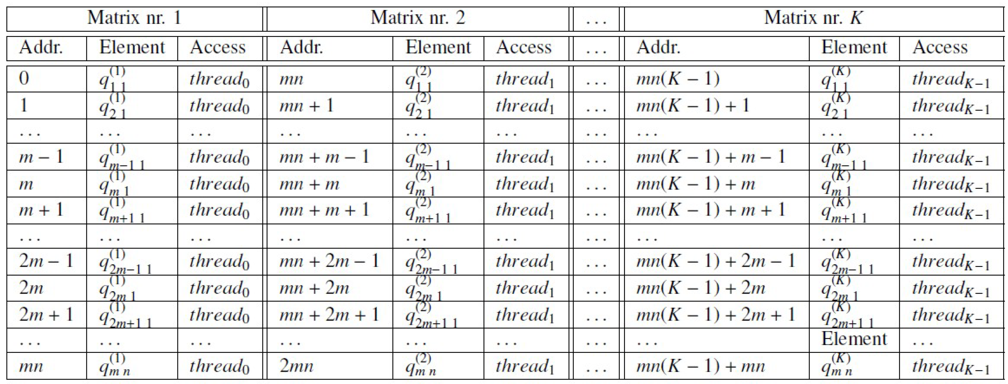
Figure 4 illustrates a natural, consecutive memory storage of the pool of matrices. With each thread assigned to a different matrix, such a storage scheme does not lead to a coalesced memory access since consecutive threads do not access consecutive regions of memory. Opposite to that, a more performing data organization, which has been used in this paper, consists of an interlaced matrix storage as illustrated in Figure 5. In this case, parallel threads running the same instruction access consecutive locations of global memory, leading to a far higher memory bandwidth.
In other words, Figure 4 demonstrates how naïve back-to-back storage causes each warp to fetch scattered addresses, leading to under-utilized memory transactions. By contrast, Figure 5’s interlaced layout aligns consecutive thread IDs with consecutive addresses, enabling full 128-byte coalesced reads. To better clarify this point, Figure 6a illustrates K input matrices stored one after another as K stacks of bricks, where each brick is one matrix. In the conventional layout, continuous GPU threads uselessly pick up inhomogeneous stacks, and memory transactions fetch many unused words. In the interlaced layout illustrated in Figure 6b, the bricks are redistributed so that each thread takes homogeneous bricks. In other words, threads in a warp access consecutive bricks, all of which are used, yielding coalesced global-memory reads.
According to what the above said, and in order to interface the natural input storage of Figure 4 to that of Figure 5, the __global__ function in Algorithm 2 is employed.
Algorithm 2 Memory reorganization __global__ function.
__global__void  r e o r g a n i z e (double * i n , double * o u t , int
                                              K, int  r o w s , int  c o l s ) {
      int  t i d = t h r e a d I d x . x + b l o c k D i m . x b l o c k I d x . x ;
      if  ( t i d < K )
          for (int  i = 0 ; i < r o w s ; i ++)
               for (int  j = 0 ; j < c o l s ; j ++)
                   o u t [ t i d + j K + i K c o l s ] =
                     i n [ t i d r o w s c o l s + j r o w s + i ] ; }

3.2. Thread-Level and Instruction-Level Parallelism

Before describing the parallelization strategies devised for steps 1 through 3, we mention the opportunity of using thread-level parallelism or instruction-level parallelism.
The achievable level of thread parallelism with very tiny matrices, as in the case discussed in the present work, is very low due to the organization of the execution pattern on the GPU. Accordingly, the parallelization strategies for steps 1 through 3 will rely much on the exploitation of instruction-level parallelism.

3.3. Parallelization of the First Step (Bidiagonalization)

Computing the bidiagonalization with the scheme discussed in Section 2.1, namely, using a series of Householder transformations, has two main drawbacks for parallel implementation on GPUs.
The first, most evident drawback is the data dependency between each bidiagonalization step. Indeed, the right lower ( m i ) × ( n i ) submatrix of A i obtained at the ith iteration step of the procedure is the starting point for the calculation of the submatrix A i + 1 at the ( i + 1 ) th step.
The second issue concerns the continuous reduction of the matrix size against the step index i, which implies that each iteration operates on a smaller input matrix as compared to the previous one. Accordingly, a continuous reduction of the workload takes place. Continuously reducing the workload is an issue for parallel implementations on GPUs since it is likely to prevent saturating the computational resources of the device.
Furthermore, concerning the matrix update involved in Equation (10), it should be mentioned that the popular approach in [46] partitions the input matrix into square blocks. Assuming that L is the dimension of each block, the matrix update occurs only after L rows and L columns have been bidiagonalized. In this way, the matrix update is deferred, avoiding the update after each row-column elimination which involves many read/write memory operations. Unfortunately, this approach has been devised for large matrices and is not suitable for matrices as small as those dealt with in this paper.
Following the above considerations and the one in the foregoing subsection, in our approach, each thread is in charge of computing the whole bidiagonalization for a single matrix. Therefore, if K is the size of the pool of matrices, the kernel launch configuration is organized as a one dimensional grid of thread blocks with a fixed number of threads per block equal to B L O C K S I Z E and a number of blocks equal to the smallest integer not smaller than K / B L O C K S I Z E .
The bidiagonalization step has been implemented by the kernel function reported in Algorithm 3. computeLeftHouse and computeRightHouse are __device__ calculating left and right Householder’s vectors, respectively, according to Section 2.1.
Algorithm 3 Bidiagonalization __global__ function.
__global__void  b i d i a g (double * i n , int m a x i t , int K, int r o w s , int c o l s ) {
     int  t i d = t h r e a d I d x . x + b l o c k D i m . x b l o c k I d x . x ;
       double  l e f t H o u s e [ m a x r o w s ] , r i g h t H o u s e [ m a x c o l s ] , h [ m a x c o l s ] , w i [ m a x r o w s ] , x i [ m a x c o l s ] , z i [ m a x c o l s ] ;
     double  b e t a u = b e t a v = 0 . , s u m ;
     for (int  c o u n t = 0 ; c o u n t < m a x i t ; c o u n t ++) {
         if ( c o u n t < c o l s 2 ) {
                 if ( t i d < K ) {
                   c o m p u t e L e f t H o u s e ( i n , l e f t H o u s e , b e t a u , t i d , c o u n t , K, r o w s , c o l s );
                   for (int  j = 0 ; j < c o l s ; j ++) {
                     s u m = 0 . ;
                     for (int  i = 0 ; i < r o w s ; i ++) s u m + = b e t a u l e f t H o u s e [ i ] i n [ t i d + i K c o l s + j K ] ;
                     h [ j ] = s u m + i n [ t i d + j K + c o u n t K c o l s ] ;
                     x i [ j ] = s u m ; }
                   c o m p u t e R i g h t H o u s e (h, r i g h t H o u s e , b e t a v , t i d , c o u n t , K, r o w s , c o l s );
                   for (int  i = 0 ; i < r o w s ; i ++) {
                     s u m = 0 . ;
                     for (int  j = 0 ; j < c o l s ; j ++) s u m + = b e t a v r i g h t H o u s e [ j ] i n [ t i d + i K c o l s + j K ] ;
                     w i [ i ] = s u m ; }
                   s u m = 0 . ;
                   for (int  i = 0 ; i < c o l s ; i ++) s u m + = x i [ i ] r i g h t H o u s e [ i ] ;
                   for (int  i = 0 ; i < c o l s ; i ++) z i [ i ] = x i [ i ] b e t a v s u m r i g h t H o u s e [ i ] ;
                   for (int  r = 0 ; r < r o w s ; r ++)
                     for (int  c = 0 ; c < c o l s ; c ++) i n [ t i d + r K c o l s + c K ] = l e f t H o u s e [ r ] z i [ c ] ; }}
                 if ( c o u n t > = c o l s 2 ) {
                   if ( t i d < K ) {
                   c o m p u t e L e f t H o u s e ( i n , l e f t H o u s e , b e t a u , t i d , c o u n t , K, r o w s , c o l s );
                   for (int  j = 0 ; j < c o l s ; j ++) {
                     double  s u m = 0 . ;
                     for (int  i = 0 ; i < r o w s ; i ++) s u m + = l e f t H o u s e [ i ] i n [ t i d + i K c o l s + j K ] ;
                     x i [ j ] = s u m ; }
                   for (int  r = 0 ; r < r o w s ; r ++)
                     for (int  c = 0 ; c < c o l s ; c ++) i n [ t i d + r K c o l s + c K ] = b e t a u x i [ c ] l e f t H o u s e [ r ] + i n [ t i d + r K c o l s + c K ] ; } } } }

3.4. Parallelizations of the Second (Tridiagonalization) and Third (Root Finding) Steps

Step 2, namely tridiagonalization, is trivially implemented as a __device__ function in CUDA, so that this point will be here skipped.
Following the considerations in Section 2.3 about the embarrassingly level of parallelism of the third step, the bisection algorithm is executed on a 2D grid of threads, with the threads along the x dimension assigned to a different matrix and the threads along the y dimension in charge of calculating a single eigenvalue of each matrix.
The bisection approach is implemented by the kernel function reported in Algorithm 4. The functions chcksign, pivot, tridiag, and initInterv appearing there are __device__ functions. In particular, chcksign and pivot implement the Count function (see Appendix A), tridiag calculates the elements of the tridiagonal matrix, and initInterv calculates the initial search interval for bisection.
Algorithm 4 Bisection __global__ function.
__global__void  b i s e c t i o n (double * d, double * b, double *  d d , double * b b , double * S V , int K, int  c o l s , double  t o l ) {
        int  t i d x = t h r e a d I d x . x + b l o c k D i m . x b l o c k I d x . x ;
        int  t i d y = t h r e a d I d x . y ;
        double  a l p h a , b e t a , p i v o t ;
          __shared__double   a l p h a s h a r e d [ b l o c k S i z e S t u r m ] , b e t a s h a r e d [ b l o c k S i z e S t u r m ] , p i v m i n s h a r e d [ b l o c k S i z e S t u r m ] ;
        if ( t i d x < K && t i d y = = 0 ) {
            t r i d i a g ( d + t i d x , b + t i d x , d d + t i d x , b b + t i d x , K, c o l s );
            p i v o t ( b b + t i d x , & p i v m i n s h a r e d [ t h r e a d I d x . x ] , K, c o l s );
            i n i t I n t e r v ( d d + t i d x , b b + t i d x , a l p h a s h a r e d [ t h r e a d I d x . x ] , b e t a s h a r e d [ t h r e a d I d x . x ] , K, c o l s ); }
        __syncthreads();
        if ( t i d x < K && t i d y < c o l s ) {
          int  e i g I n d e x = t i d y % c o l s ;
            int  n u m C h a n g e s = 0 ;
            double  c = 0 ;
            a l p h a = a l p h a s h a r e d [ t h r e a d I d x . x ] ;
            b e t a = b e t a s h a r e d [ t h r e a d I d x . x ] ;
            p i v o t = p i v m i n s h a r e d [ t h r e a d I d x . x ] ;
            double  d i s t = f a b s ( b e t a a l p h a ) ;
            double  s = f a b s ( b e t a ) + f a b s ( a l p h a ) ;
            while ( d i s t > t o l s ) {
                c = ( a l p h a + b e t a ) / 2 . ;
                c h c k s i g n ( d d + t i d x , b b + t i d x , p i v o t , c, n u m C h a n g e s , K, c o l s );
                if  ( n u m C h a n g e s > ( c o l s ( e i g I n d e x + 1 ) ) ) b e t a = c ;
                else  a l p h a = c ;
                d i s t = f a b s ( b e t a a l p h a ) ;
                s = f a b s ( b e t a ) + f a b s ( a l p h a ) ; }
            S V [ e i g I n d e x + t i d x c o l s ] = s q r t ( f a b s ( c ) ) ; } }

3.5. Multi-GPU Processing

The multi-GPU processing is implemented by distributing the overall number K T of matrices to be processed on the available N G P U GPUs. In this way, each GPU operates on a number of K = K T / N G P U matrices. The data transfers towards the GPUs is performed by asynchronous copies using cudaMemcpyAsync to make them occur concurrently.

3.6. Computational Complexity and Memory Requirements Per-Thread

3.6.1. Bidiagonalization

The cost of the bidiagonalization via Householder reflections step per matrix, namely, per thread, is ( m · n 2 )  [47]. The GPU global memory requirement per-thread in bytes is ( m ( n + 2 ) 1 ) μ ( T ) , where μ ( T ) = 4 for single precision or μ ( T ) = 8 for double precision. The GPU local per thread register/stack memory requirement is ( 3 m + 4 n ) μ ( T ) .

3.6.2. Tridiagonalization

The cost of the tridiagonalization step is ( m + n ) . The GPU global memory requirement per thread in bytes is 2 ( m + n ) μ ( T ) .

3.6.3. Root-Finding by Sturm Bisection

The cost of the root-finding by bisection with Sturm sequences per matrix is O ( n log ( W / δ ) ) , where W is the Gershgorin-interval width and δ the tolerance. The GPU global memory requirement per thread in bytes is ( m + 2 ( n + 1 ) ) μ ( T ) .

3.7. Comparison with the Approaches in [14,22,23]

The approach in [22] has a computational complexity of ( S m n 2 ) , where S is the number of sweeps which can be, in the worst case, log ( n ) . Opposite to that, the computational complexity of the scheme in [23] is ( m n 2 ) . Finally, for square matrices, the approach in [14] is ( n 3 ) .

4. Numerical Results

In this section, we present some of the results of an extensive numerical analysis aimed at assessing the performance of the proposed approach. Although the CUDA code has been implemented in both single- and double-precision arithmetics, double precision is mainly considered here, with most of the trends for single precision being similar.
Performance is assessed against a different size K T of the batch to be processed. In particular, for all the examples below, K T = 2 n , n = 4 , , 20 . In this way, either the case of a small and of a large number of matrices can be dealt with. Furthermore, we consider the case of either square or rectangular matrices. In the rectangular case, we set m = n 2 to have again the possibility to evaluate the performance for an increasing matrix size. Below, we separate the analysis between the cases of single-GPU and multi-GPU processing.
We finally underline that the GPU timings below include the bidirectional host-device memory transfers. The plots are all reported in log-log scale.
The assessment has been performed on different single- and multi-GPU architectures. We will firstly consider the case of a g4dn.12xlarge AWS instance (Amazon SageMaker) comprising 48 vCPUs, CPUs of the Intel Xeon Family, 192 GB of memory, 4 NVIDIA T4 Tensor Core GPUs of compute capability 7.5 , and 64 GB of global memory. The employed CUDA version has been 12.2 and the code has been compiled with the O 3 optimization option.

4.1. Accuracy, Runtime, and Stability

Before assessing the computational performance of the technique, we analyze its accuracy and stability. In particular:
  • we quantify the effect of the tolerance parameter δ on both accuracy and runtime;
  • we assess the robustness of the method on ill-conditioned matrices;
  • we assess the robustness of the method against noisy matrices.

4.1.1. Percentage Root Mean Square Error

Let A be an m × n test matrix, σ = { σ i } the vector of the singular values computed by our approach, and σ ^ = { σ ^ i } the reference singular values. The percentage relative root mean square SV error (PRMSE) is computed as
E RMSE = 100 · σ σ ^ 2 σ ^ 2 ,
where · 2 denotes the standard quadratic norm.

4.1.2. Tolerance Against Accuracy and Runtime

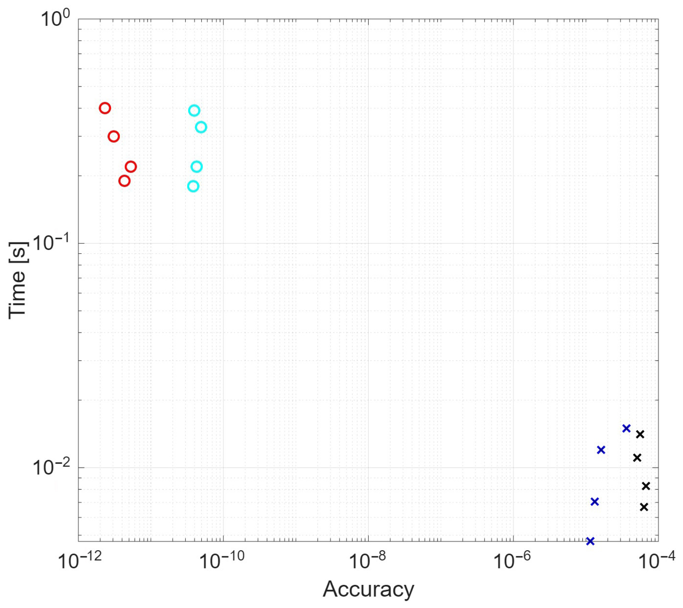
Figure 7 shows an accuracy/runtime map for single- and double-precision arithmetic for random Gaussian matrices having 3 × 3 , 4 × 4 , 5 × 5 , and 6 × 6 sizes and for different tolerance parameters δ . In particular, δ = 10 6 and δ = 10 7 have been dealt with for single-precision, while δ = 10 12 and δ = 10 13 have been considered for double-precision. As can be seen, the resulting RMSE agrees with the typical tolerances of the two kinds of arithmetic, and, of course, more accuracy is paid with a larger computation time.

4.1.3. Stability Against the Condition Number

We have considered 4 × 4 Gaussian random matrices with different condition numbers and double-precision arithmetics, having fixed δ = 10 13 . In particular, the matrices have condition numbers D = 10 κ , with κ { 2 , 4 , 6 , 8 , 10 } , and have been defined by generating random singular vector matrices and singular values d i = 10 κ ( i 1 ) / ( m 1 ) , i = 0 , , m 1 . Table 1 summarizes the results of the analysis and shows how the PRMSE keeps tolerable even for very highly ill-conditioned matrices.

4.1.4. Noise Perturbation

Finally, to probe sensitivity to noise, we have considered noisy, 4 × 4 matrices using A noisy = A + ϵ A 2 G , with G Gaussian and ϵ { 10 8 , 10 7 , 10 6 , 10 5 } , again with double-precision arithmetic and δ = 10 13 . Table 2 resumes the stability of the algorithm against the noise.

4.2. Performance of the Approach for the Single GPU Case

Figure 8 illustrates the processing time for the proposed approach when only 1 GPU is employed. The processing time is reported against the number of matrices and parameterized on the size of the involved matrices. The template version of the code has been run with a tolerance δ chosen equal to 10 7 . It can be seen that, unless the batch saturates the GPU resources, which occurs for K T 1024 , the processing time does not significantly change with the batch size.
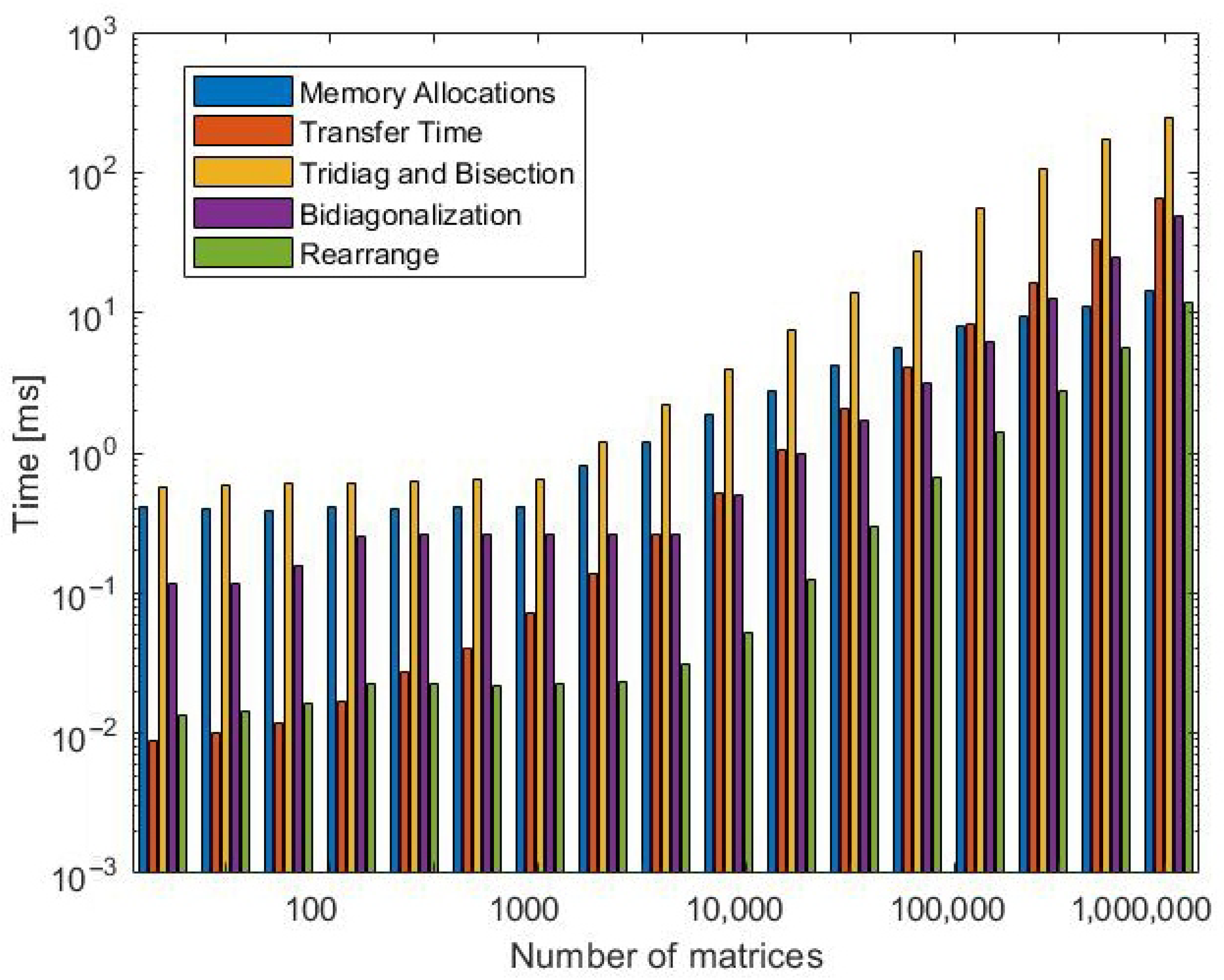
Figure 9, on the other side, illustrates the separate timings of the different algorithm stages. It highlights how the most computationally expensive stage is represented by the tridiagonalization and bisection one.
We have also confronted our scheme with a fully CPU one based on the use of the parallel, CPU multicore Intel MKL library [10]. Comparing the proposed approach with a multicore CPU implementation has a rationale in the fact that multicore CPUs are often perceived as the best computing platform for such kinds of computational problems, namely, computations on very large numbers of small items. However, also in this case, our algorithm has outperformed the compared one.
We now want to illustrate the speedup obtained by the above-discussed template implementation of the code. More in detail, as can be seen from Figure 10, the template version enables gaining about 10 % of the overall processing time against the non-template version of the approach.
We finally want to show, in Figure 11, how the algorithm performs for non-square matrices. As it can be seen, there is no significant performance loss due to the rectangularity of the matrices. Also, we have compared the computing time of the case when δ = 10 7 against the case δ = 10 9 . A performance loss of about 10 % has been observed, which is definitely tolerable in applications requiring more accuracy: despite the requested accuracy improvement of two orders of magnitude, the case δ = 10 7 is not much faster than the case δ = 10 9 .
Finally, Table 3 reports the root-mean-square (RMS) errors of the singular values computed by our GPU-based method versus MATLAB’s state-of-the-art svd reference, for square matrices with sizes from 2 × 2 to 8 × 8 , and for two tolerance levels for double precision arithmetic, namely, δ = 10 7 and δ = 10 9 , and for a single tolerance level for single-precision arithmetic, namely, δ = 10 4 . Furthermore, Table 3 also reports the RMS errors for some rectangular matrices for δ = 10 7 and double precision arithmetic only. For each size in the square matrices case, we also include the RMS errors obtained with Intel MKL’s desvg routine under its default settings. As shown, when δ = 10 7 , our approach already achieves < 10 12 RMS errors, closely matching MATLAB’s results. Tightening the tolerance to δ = 10 9 reduces the RMS error further—dropping below 10 16 and outperforming MKL. This demonstrates that our bisection-based solver not only meets the accuracy of established CPU routines but also allows explicit control of precision via the δ parameter without significant loss of robustness.

4.3. Performance of the Approach in Comparison to cuSOLVER’s Gesvd

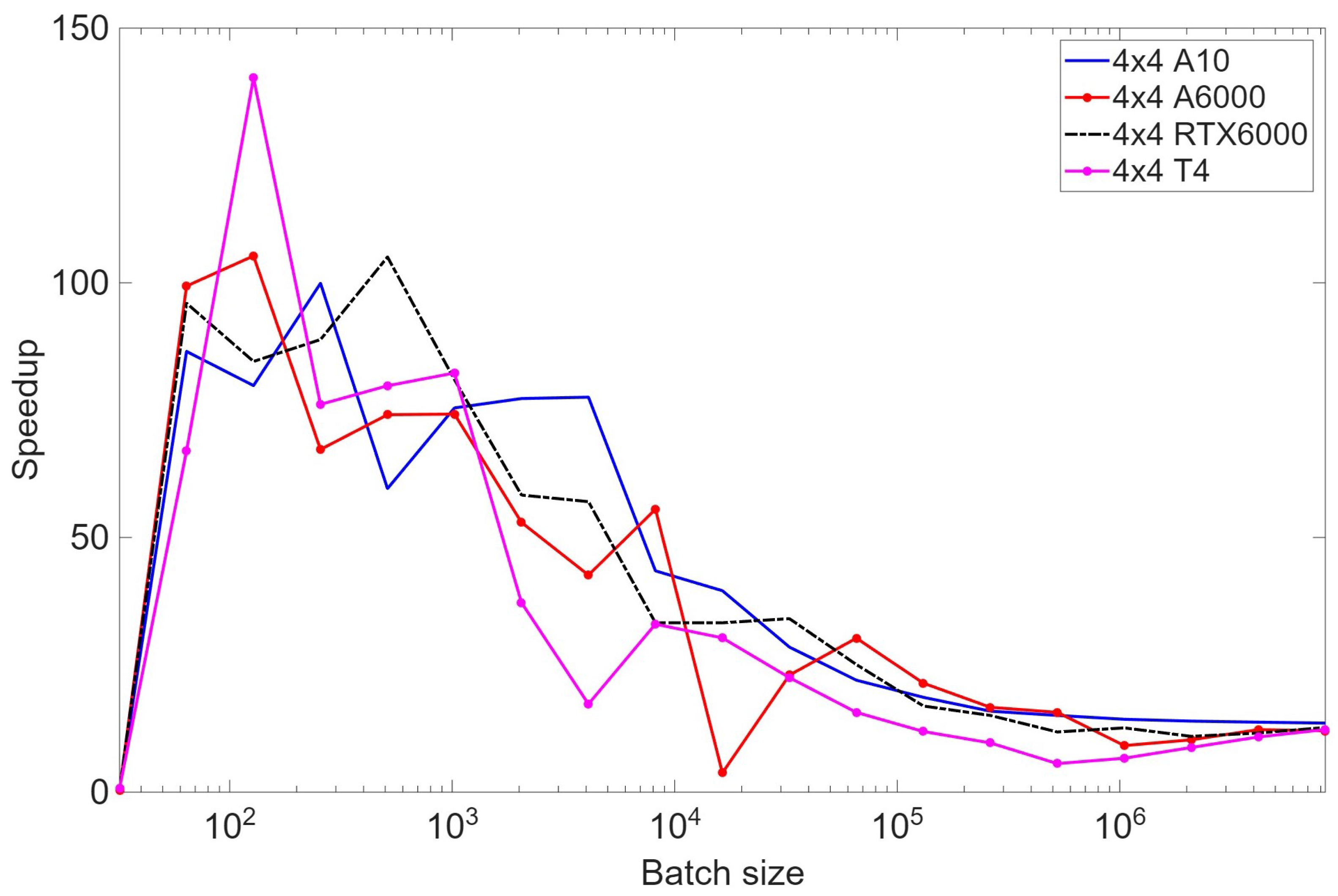
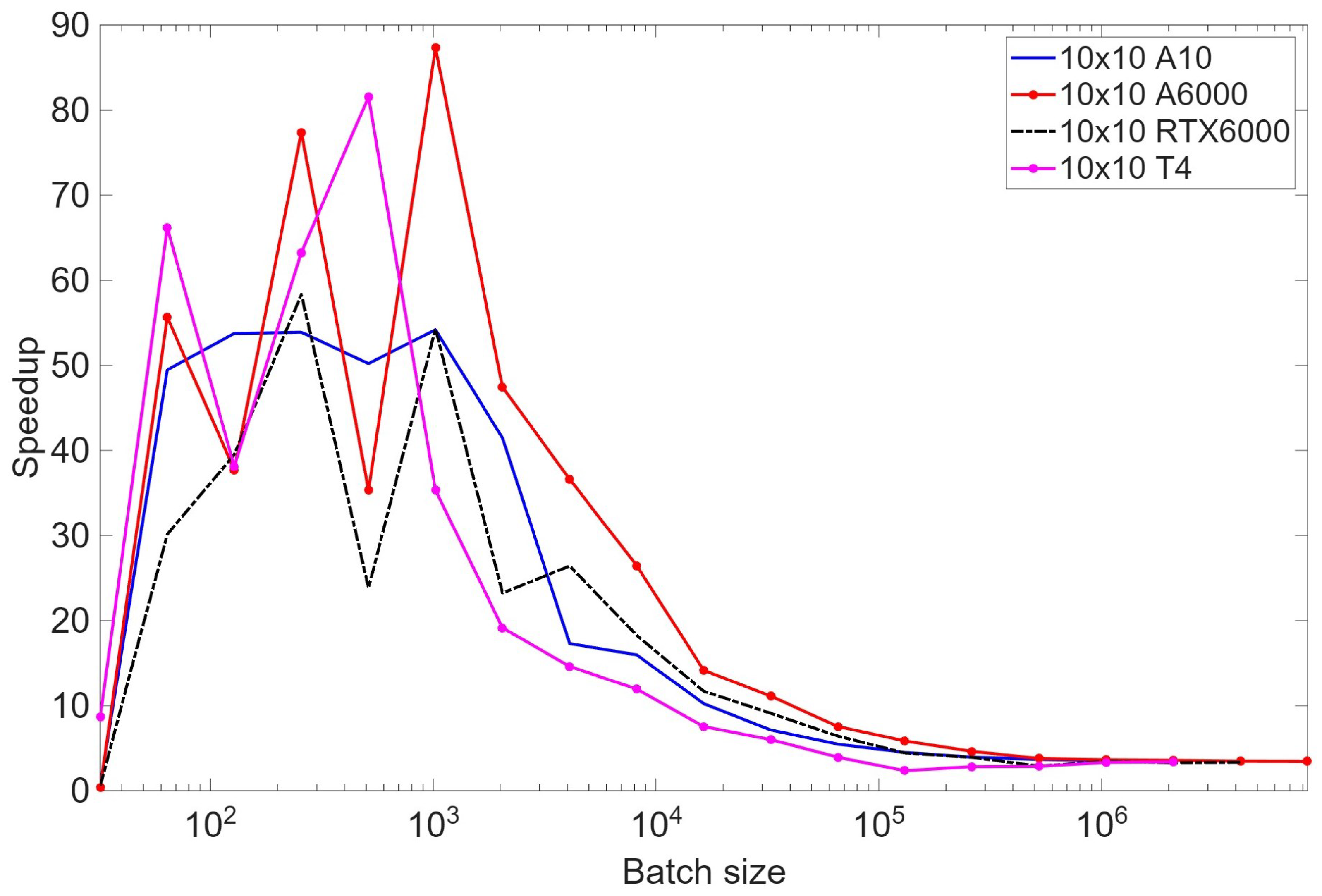
The performance of the approach is further compared to cuSOLVER’s gesvd routine on four different GPUs, namely, A10, A6000, RTX6000, and T4, for the case of double precision arithmetic. In particular, Figure 12 and Figure 13 illustrate the speedup experienced when using the proposed numerical scheme for 4 × 4 and 10 × 10 matrices in the case of double precision arithmetic. The advantage of our technique is highlighted by a speedup reaching 20 for batches of 4 × 4 matrices and 3.5 for batches of 10 × 10 matrices. The PRMSE in our case has been around 4 × 10 12 , while that for cuSOLVER’s gesvd routine has been also lower settling down around 3 × 10 7 . We notice that cuSOLVER’s gesvd forms the basis for several, publicly available routines as current versions of JAX, PyTorch, and CuPy.

4.4. Performance of the Approach for the Multi-GPU Case

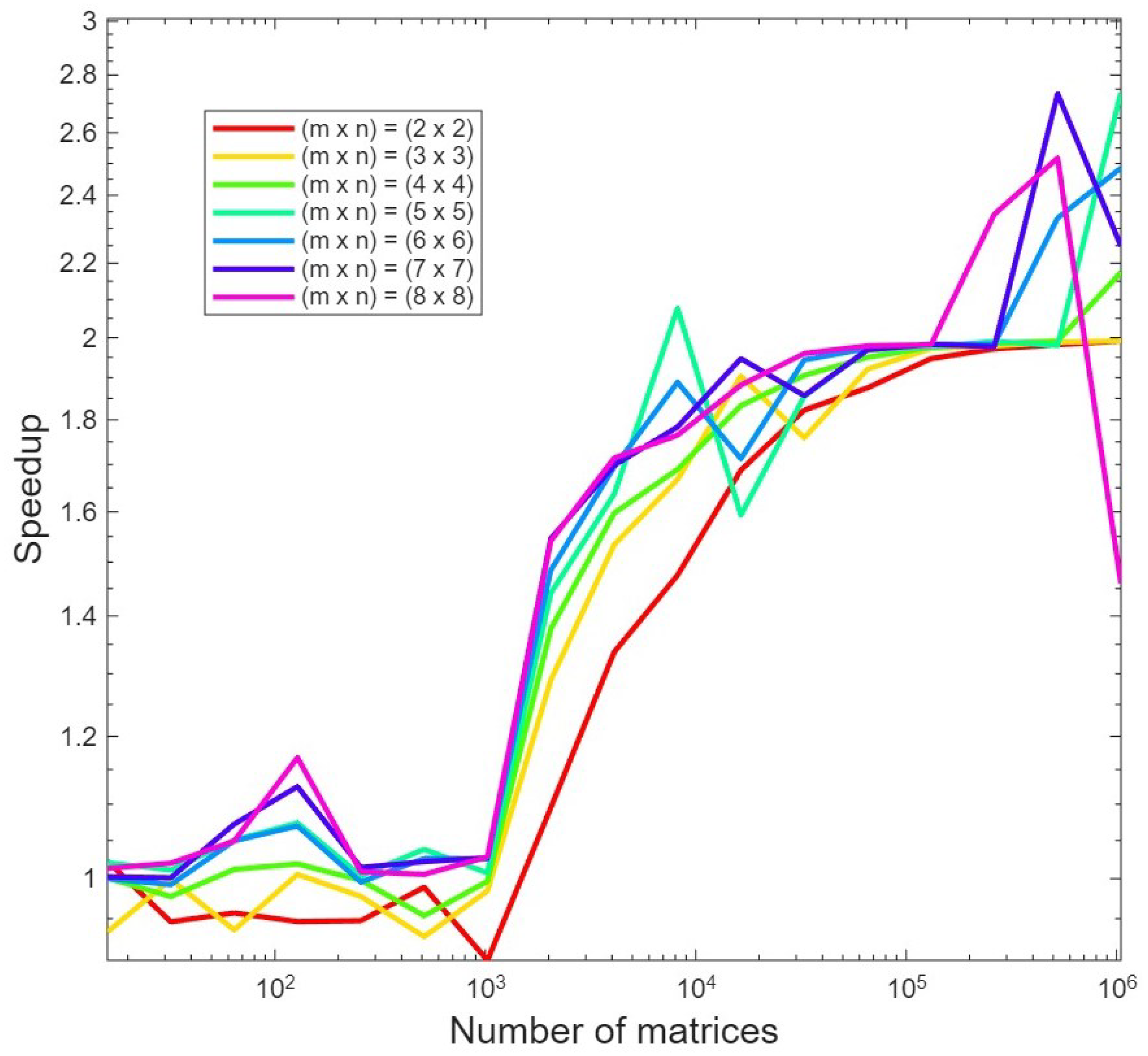
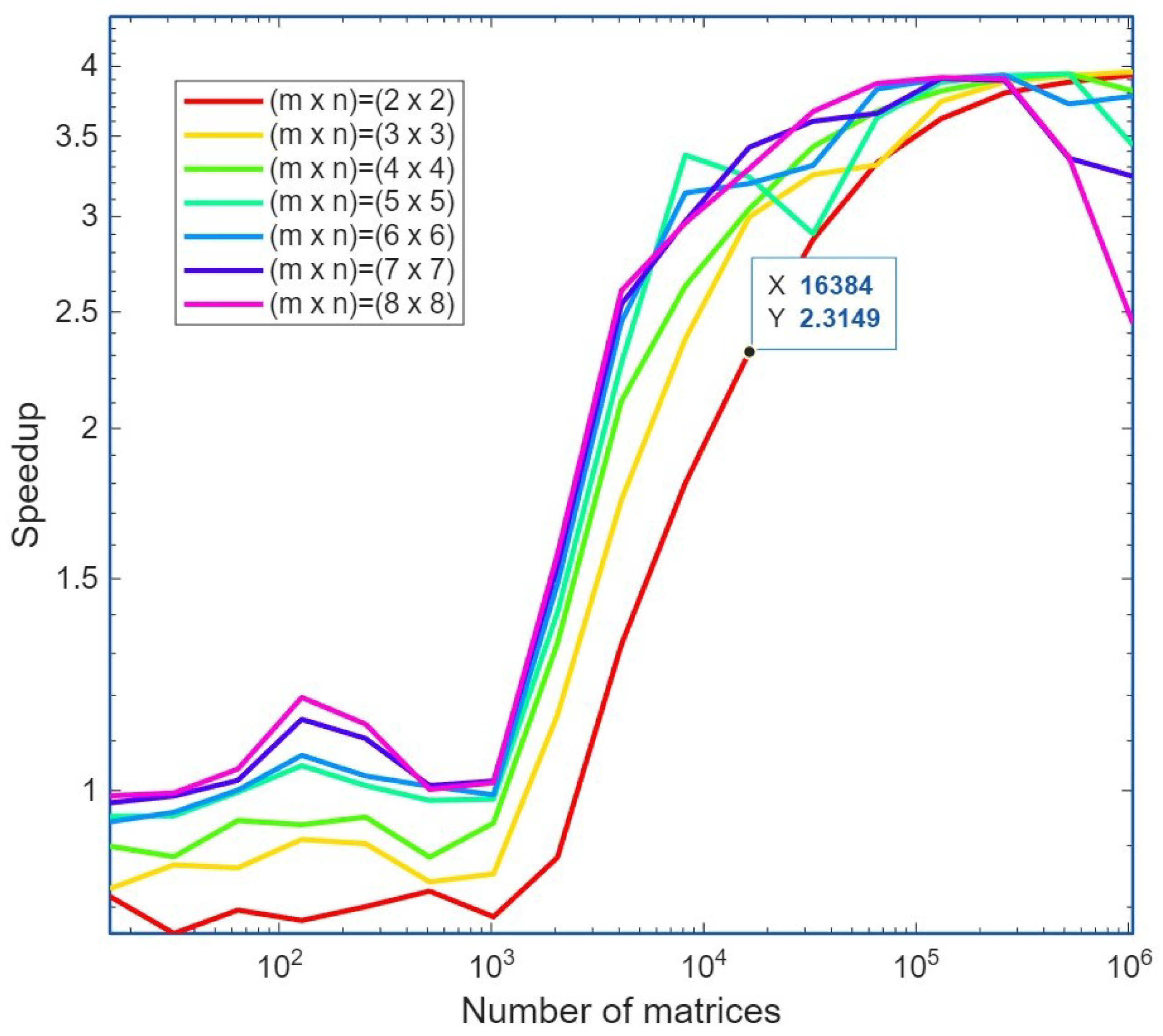
Finally, in order to assess the scaling capabilities of our scheme in the multi-GPU case, Figure 14 and Figure 15 show the speedup achieved against the single-GPU case when 2 or 4 GPUs are employed, respectively. As can be seen, once the GPU resources have been saturated, scalings of about 2 and 4 are observed for the two cases.
To further confirm the scaling features of the approach, we have tested it against a dual-GPU system based on NVIDIA A6000 cards. More in detail, we have considered a batch of 10 23 matrices. The case of 4 × 4 matrices run in 0.32 s on a single GPU and in 0.16 s on two GPUs, while the case of 10 × 10 matrices took 2.25 s to run on a single GPU and 1.13 s to complete the processing on two GPUs, thus confirming the good scaling features of our approach.

5. Conclusions and Future Developments

A fast and robust approach to evaluate the singular values of small matrices on Graphics Processing Units (GPUs) was presented, exploiting interlaced storage, bidiagonalization via Householder transformations, symmetric tridiagonalization, and Sturm-sequence–based bisection. The algorithm was implemented in CUDA and tested on several single- and multi-GPU architectures. For large matrix batches, the speed-up against cuSOLVER’s gesvd has been around 20 for 4 × 4 matrices. Furthermore, near-linear scaling across the GPUs ( 4 × acceleration) has been yielded, while maintaining an RMS error below 2.3 × 10 7 in single precision for relative tolerance δ = 10 4 and below 2.3 × 10 13 in double precision for δ = 10 7 . By tightening the tolerance to δ = 10 9 , RMS errors dropped below 2 × 10 13 , thus matching the accuracy of MATLAB’s state-of-the-art svd routine and demonstrating that, with proper choice of δ , the proposed method can achieve precision equivalent to MATLAB’s svd. Furthermore, tightening the tolerance from δ = 10 7 to δ = 10 9 increased the total runtime by only about 10%. It was also verified that the performance in terms of execution time for rectangular matrices did not differ significantly as compared to the square matrices case. Future developments include extension to complex matrices and application to large-scale singular value optimization problems. Steps of the algorithm requiring the computation of matrix multiplications can also be further improved using approaches specifically tailored to small matrices as in [14].

Author Contributions

Conceptualization, A.C., C.C., S.D.D. and A.L.; Methodology, A.C., C.C., S.D.D. and A.L.; Software, A.C., C.C., S.D.D. and A.L.; Validation, A.C., C.C., S.D.D. and A.L.; Formal analysis, A.C., C.C., S.D.D. and A.L.; Investigation, A.C., C.C., S.D.D. and A.L.; Resources, A.C., C.C., S.D.D. and A.L.; Data curation, A.C., C.C., S.D.D. and A.L.; Writing—original draft, A.C., C.C., S.D.D. and A.L.; Writing—review & editing, A.C., C.C., S.D.D. and A.L.; Visualization, A.C., C.C., S.D.D. and A.L.; Supervision, A.C., C.C., S.D.D. and A.L.; Project administration, A.C., C.C., S.D.D. and A.L.; Funding acquisition, A.C., C.C., S.D.D. and A.L. All authors have read and agreed to the published version of the manuscript.

Funding

This work has been partially supported by the Spoke 9 Digital Society & Smart Cities of ICSC—Centro Nazionale di Ricerca in High-Performance-Computing, Big Data and Quantum Computing, funded by European Union—NextGenerationEU (PNRR-HPC, CUP: E63C22000980007).

Data Availability Statement

The original contributions presented in this study are included in the article. Further inquiries can be directed to the corresponding author.

Conflicts of Interest

The authors declare no conflicts of interest.

List of Abbreviations

AWSAmazon Web Services
CUDACompute Unified Device Architecture
GPUGraphics Processing Unit
MKLIntel Math Kernel Library
MIMOMultiple-Input/Multiple-Output
RMSroot-mean-square
SVDSingular Value Decomposition

Appendix A

A trivial implementation of the Count(x) function is reported in Algorithm A2, where β 0 = 0 has been assumed.
However, turning Algorithm A2 to a stable function requires:
  • handling the division by zero;
  • preserving the monotonicity.
A solution to the first problem has been given in [27]. First, a proper scaling of the input matrix is performed to avoid that its largest element approaches the overflow threshold. Then, the pivot d (see Algorithm A2) is moved away from zero by a small quantity pivmin = 2 B / Ω , where B = m a x i j ( 1 , T i j 2 ) and Ω is the overflow threshold. This pivmin version of Count(x) is also used in the LAPACK’s dstebz routine and it is reported in Algorithm A1.
Regarding the latter problem, in exact arithmetics Count(x) grows monotonically with x. This is not always true in floating point arithmetics, i.e., even if x 1 < x 2 , the computer implementation might report C o u n t ( x 1 ) > C o u n t ( x 2 ) , so that the interval [ x 1 , x 2 ) would appear to contain a negative number of eigenvalues. However, if an overflow-safe implementation of Count(x) is used (as the pivmin version), and if the arithmetics is monotonic (as the IEEE754 implemented by the GPUs also), then also the floating point implementation of Count(x) is a monotonically increasing function of x for a symmetric tridiagonal matrix [27,48]. A deep and detailed analysis about correct sequential and parallel floating point implementations of bisection-like methods for solving the eigenvalue problem for the more generally symmetric acyclic matrices can be found in [27].
Algorithm A1  c o u n t ( x ) - pivmin version.
c o u n t = 0 ;
d = 1 ;
for  i = 1 : n do
       d = α i x β i 1 2 / d ;
       if  | d | < p i v m i n  then
        d = p i v m i n ;
       end
       if  d < 0  then
        c o u n t = c o u n t + 1 ;
       end
end
Algorithm A2  c o u n t ( x ) .
c o u n t = 0 ;
d = 1 ;
for  i = 1 : n do
       d = α i x β i 1 2 / d ;
       if  d < 0  then
        c o u n t = c o u n t + 1 ;
       end
end

References

  1. Bertero, M.; Boccacci, P. Introduction to Inverse Problems in Imaging; Institute of Physics Publishing: Bristol, UK, 1998. [Google Scholar]
  2. Hua, Y.; Liu, W. Generalized Karhunen-Loeve transform. IEEE Signal Proc. Lett. 1998, 5, 141–142. [Google Scholar]
  3. Bavirisetti, D.P.; Dhuli, R. Fusion of infrared and visible sensor images based on anisotropic diffusion and Karhunen–Loeve Transform. IEEE Sensors J. 2016, 16, 203–209. [Google Scholar] [CrossRef]
  4. Narwaria, M.; Lin, W. SVD-based quality metric for image and video using machine learning. IEEE Trans. Syst. Man Cybern.-Part B Cybern. 2012, 42, 347–364. [Google Scholar] [CrossRef] [PubMed]
  5. Swaminathan, S.; Garg, D.; Kannan, R.; Andres, F. Sparse low rank factorization for deep neural network compression. Neurocomputing 2020, 398, 185–196. [Google Scholar] [CrossRef]
  6. Capozzoli, A.; Curcio, C.; D’Elia, G.; Ferrara, F.; Gennarelli, C.; Guerriero, R.; Liseno, A. A probe-compensated helicoidal NF-FF transformation for aperture antennas using a prolate spheroidal expansion. Int. J. Antennas Prop. 2012, 2012, 753156. [Google Scholar] [CrossRef]
  7. Capozzoli, A.; Curcio, C.; Liseno, A. Singular Value Optimization in inverse electromagnetic scattering. IEEE Antennas Wirel. Prop. Lett. 2017, 16, 1094–1097. [Google Scholar] [CrossRef]
  8. Xiong, Y.; Liang, B.; Yu, H.; Chen, J.; Jin, Y.; Xing, M. Processing of bistatic SAR data With nonlinear trajectory using a controlled-SVD algorithm. IEEE J. Sel. Top. Appl. Earth Obs. Remote Sens. 2021, 14, 5750–5759. [Google Scholar] [CrossRef]
  9. Breglia, A.; Capozzoli, A.; Curcio, C.; Donna, S.D.; Liseno, A. GPU-based electromagnetic optimization of MIMO channels. ACES Express J. 2018, 33, 172–175. [Google Scholar]
  10. Capozzoli, A.; Curcio, C.; Donna, S.D.; Liseno, A. Massive computation of singular values of small matrices on GPUs. In Proceedings of the IEEE Computational Electromagnetics International Workshop (CEM), Izmir, Turkey, 1–4 July 2015; pp. 36–37. [Google Scholar]
  11. Messer, O.E.B.; Harris, J.A.; Parete-Koon, S.; Chertkow, M.A. Multicore and accelerator development for a leadership-class stellar astrophysics code. In Applied Parallel and Scientific Computing; Manninen, P., Ed.; Springer: Berlin/Heidelberg, Germany; pp. 92–106.
  12. Sedghi, H.; Gupta, V.; Long, P.M. The singular values of convolutional layers. In Proceedings of the 7th International Conference on Learning Representations, New Orleans, LA, USA, 6–9 May 2019; pp. 1–12. [Google Scholar]
  13. Jia, K.; Tao, D.; Gao, S.; Xu, X. Improving training of deep neural networks via Singular Value Bounding. In Proceedings of the IEEE Conference on Computer Vision and Pattern Recognition, Honolulu, HI, USA, 21–26 July 2017; pp. 3994–4002. [Google Scholar]
  14. Dong, T.; Haidar, A.; Tomov, S.; Dongarra, J. Accelerating the SVD bi-diagonalization of a batch of small matrices using GPUs. J. Comput. Sci. 2018, 26, 237–245. [Google Scholar] [CrossRef]
  15. Drinea, E.; Drineas, P.; Huggins, P. A randomized singular value decomposition algorithm for image processing applications. In Proceedings of the 8th Panhellenic Conference in Informatics, Nicosia, Cyprus, 8–10 November 2001; pp. 1–10. [Google Scholar]
  16. Kirk, D.B.; Hwu, W.-M. Programming Massively Parallel Processors, A Hands-On Approach, 2nd ed.; Morgan Kaufmann: Waltham, MA, USA, 2013. [Google Scholar]
  17. Breglia, A.; Capozzoli, A.; Curcio, C.; Liseno, A. CUDA expression templates for electromagnetic applications on GPUs. IEEE Antennas Prop. Mag. 2013, 55, 156–166. [Google Scholar] [CrossRef]
  18. Capozzoli, A.; Kilic, O.; Curcio, C.; Liseno, A. The success of GPU computing in applied electromagnetics. Appl. Electromagn. Soc. J. 2018, 33, 148–151. [Google Scholar]
  19. Golub, G.H.; Kahan, W. Calculating the singular values and pseudo-inverse of a matrix. SIAM J. Numer. Anal. 1965, 2, 205–224. [Google Scholar] [CrossRef]
  20. Vandebril, R.; Barel, M.V.; Mastronardi, N. A QR–method for computing the singular values via semiseparable matrices. Numer. Math. 2004, 99, 163–195. [Google Scholar] [CrossRef][Green Version]
  21. Hassan, D.A. Deep neural network-based approach for computing singular values of matrices. Sci. J. Univ. Zakho 2025, 13, 1–6. [Google Scholar] [CrossRef]
  22. Xiao, J.; Xue, Q.; Ma, H.; Zhang, X.; Tan, G. A W-cycle algorithm for efficient batched SVD on GPUs. In Proceedings of the 27th ACM SIGPLAN Symposium on Principles and Practice of Parallel Programming, PPoPP ’22, Seoul, Republic of Korea, 2–6 April 2022; Association for Computing Machinery: New York, NY, USA, 2022; pp. 465–466. [Google Scholar]
  23. Boukaram, W.H.; Turkiyyah, G.; Ltaief, H.; Keyes, D.E. Batched QR and SVD algorithms on GPUs with applications in hierarchical matrix compression. Parallel Comp. 2018, 74, 19–33. [Google Scholar] [CrossRef]
  24. Sachdev, G.S.; Vanjani, V.; Hall, M.W. Takagi factorization on GPU using CUDA. In Proceedings of the Symposium on Application Accelerators in High Performance Computing, Knoxville, Tennessee, 13–15 July 2010; pp. 1–3. [Google Scholar]
  25. Clarkson, E.; Palit, R.; Kupinski, M.A. SVD for imaging systems with discrete rotational symmetry. Opt. Express 2010, 18, 25306–25320. [Google Scholar] [CrossRef] [PubMed]
  26. Golub, G.H.; Loan, C.F.V. Matrix Computations, 3rd ed.; Johns Hopkins University Press: Baltimore, MD, USA, 1996. [Google Scholar]
  27. Demmel, J.W.; Dhillon, I.; Ren, H. On the correctness of some bisection-like parallel eigenvalue algorithms in floating point arithmetic. Electron. Trans. Numer. Anal. 1995, 3, 116–149. [Google Scholar]
  28. Hermann, E.; Raffin, B.; Faure, F.; Gautier, T.; Allard, J. Multi-GPU and multi-CPU parallelization for interactive physics simulations. In Proceedings of the European Conference on Parallel Processing, Ischia, Italy, 31 August–3 September 2010; pp. 235–246. [Google Scholar]
  29. NVIDIA. cuSOLVER Library. DU-06709-001_v11.6, February 2022. Available online: https://www.google.com/url?sa=t&source=web&rct=j&opi=89978449&url=https://docs.nvidia.com/cuda/archive/11.6.1/pdf/CUSOLVER_Library.pdf&ved=2ahUKEwiJ4sCjioSPAxWOavUHHXUEKHYQFnoECBgQAQ&usg=AOvVaw0It8ZVo3CW4ZU2r33qj4zv (accessed on 5 May 2025).
  30. Lahabar, S.; Narayanan, P.J. Singular value decomposition on GPU using CUDA. In Proceedings of the IEEE International Symposium on Parallel & Distributed Processing, Rome, Italy, 23–29 May 2009; pp. 1–10. [Google Scholar]
  31. Kotas, C.; Barhen, J. Singular value decomposition utilizing parallel algorithms on graphical processors. In Proceedings of the OCEANS MTS/IEEE KONA, Waikoloa, HI, USA, 19–22 September 2011; pp. 1–7. [Google Scholar]
  32. Golub, G.H.; Reinsch, C. Handbook Series Linear Algebra. Singular Value Decomposition and Least Squares Solutions. Numer. Math. 1970, 14, 403–420. [Google Scholar] [CrossRef]
  33. Nash, J.C. A one-sided transformation method for the Singular Value Decomposition and algebraic eigenproblem. Comput. J. 1975, 18, 74–76. [Google Scholar] [CrossRef]
  34. Hestenes, M.R. Inversion of matrices by biorthogonalization and related results. J. Soc. Ind. Appl. Math. 1958, 6, 51–90. [Google Scholar] [CrossRef]
  35. Zhao, S.; Li, R.; Tian, W.; Xiao, W.; Dong, X.; Liao, D.; Khan, S.U.; Li, K. Divide-and-conquer approach for solving singular value decomposition based on MapReduce. Concurr. Comput. Pract. Exp. 2016, 38, 331–350. [Google Scholar] [CrossRef]
  36. Drmać, Z.; Veselixcx, K. New Fast and Accurate Jacobi SVD Algorithm. I. SIAM J. Matrix Anal. Appl. 2008, 29, 1322–1342. [Google Scholar] [CrossRef]
  37. Drmać, Z.; Veselixcx, K. New Fast and Accurate Jacobi SVD Algorithm. II. SIAM J. Matrix Anal. Appl. 2008, 29, 1343–1362. [Google Scholar] [CrossRef]
  38. Zhou, B.B.; Brent, R.P. On parallel implementation of the one-sided Jacobi algorithm for singular value decompositions. In Proceedings of the Euromicro Workshop on Parallel and Distributed Processing, San Remo, Italy, 25–27 January 1995; pp. 401–408. [Google Scholar]
  39. Zhou, B.B.; Brent, R.P. A Parallel ring ordering algorithm for efficient one-sided Jacobi SVD computations. J. Parallel Distrib. Comput. 1997, 42, 1–10. [Google Scholar] [CrossRef][Green Version]
  40. Luk, F.T.; Park, H. On parallel Jacobi orderings. SIAM J. Sci. Stat. Comput. 1989, 10, 18–26. [Google Scholar] [CrossRef]
  41. Demmel, J.; Veselić, K. Jacobi’s method is more accurate than QR. SIAM J. Matrix Anal. Appl. 1992, 13, 1204–1245. [Google Scholar] [CrossRef]
  42. Wilkinson, J.H. The Algebraic Eigenvalue Problem; Oxford University Press: New York, NY, USA, 1988. [Google Scholar]
  43. Barth, W.; Martin, R.S.; Wilkinson, J.H. Calculation of the eigenvalues of a symmetric tridiagonal matrix by the method of bisection. Numer. Math. 1967, 9, 386–393. [Google Scholar] [CrossRef]
  44. Gerschgorin, S.A. Über die abgrenzung der eigenwerte einer matrix. Izv. Akad. Nauk. SSSR Ser. Fiz.-Mat. 1931, 7, 749–754. [Google Scholar]
  45. Yi, X.; Stokes, D.; Yan, Y.; Liao, C. CUDAMicroBench: Microbenchmarks to assist CUDA performance programming. In Proceedings of the IEEE International Parallel and Distributed Processing Symposium Workshops, Portland, OR, USA, 17–21 June 2021; pp. 397–406. [Google Scholar]
  46. Choi, J.; Dongarra, J.J.; Walker, D.W. The design of a parallel dense linear algebra software library: Reduction to Hessenberg, tridiagonal, and bidiagonal form. Numer. Algorith. 1995, 10, 379–399. [Google Scholar] [CrossRef]
  47. Ralha, R.M.S. A new algorithm for Singular Value Decompositions. In Proceedings of the 2nd Euromicro Workshop on Parallel and Distributed Processing, Malaga, Spain, 26–28 January 1994; pp. 240–244. [Google Scholar]
  48. Kahan, W. Accurate Eigenvalues of a Symmetric Tridiagonal Matrix; Computer Science Department Technical Report CS41; Standford University: Standford, CA, USA, July 1966. [Google Scholar]
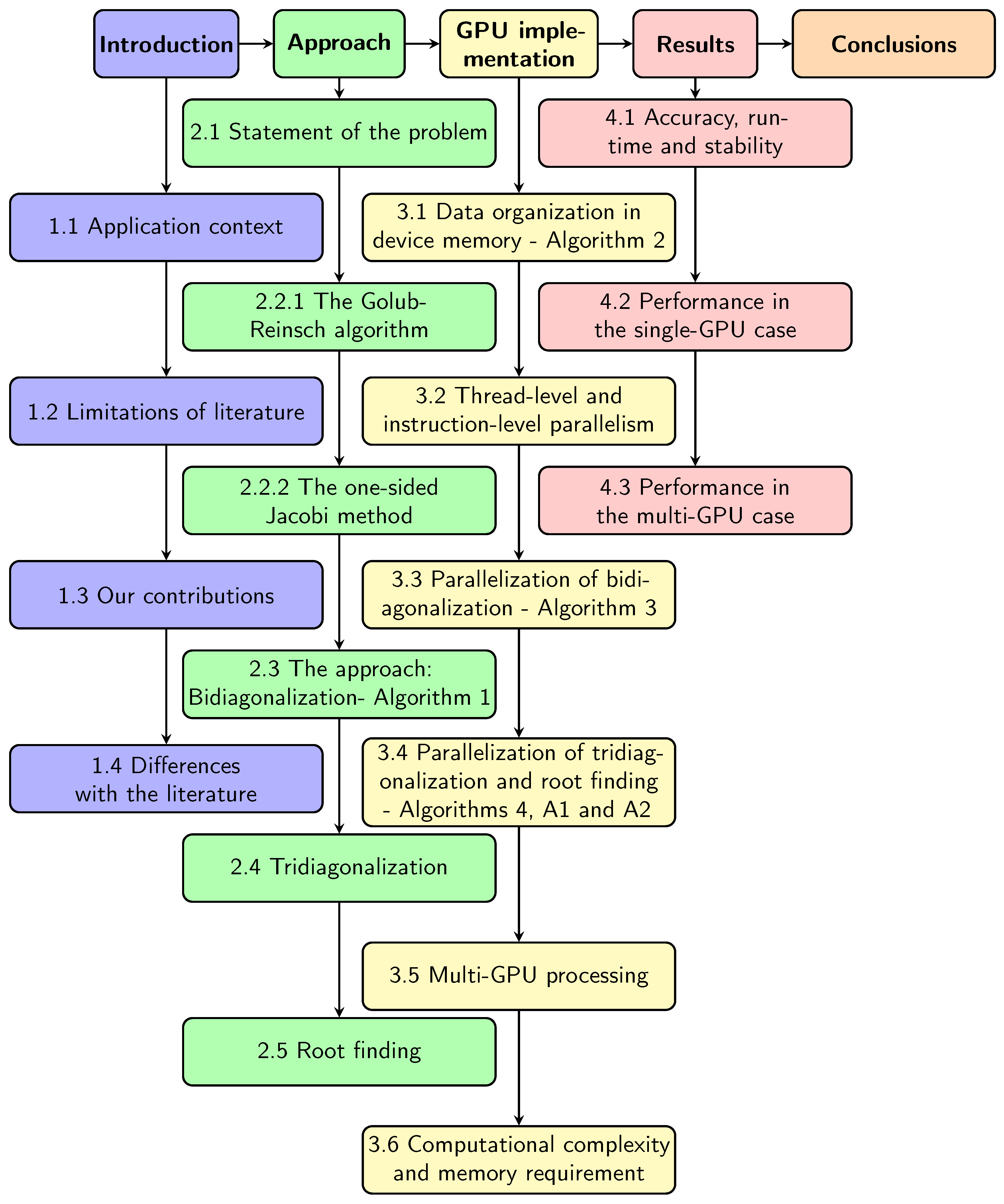
Figure 1. Paper layout.
Electronics 14 03217 g001
Figure 3. Geometric interpretation of a Householder reflection: a vector x is “folded” onto the coordinate axis by reflecting through the hyperplane orthogonal to h = x ± x e 1 .
Electronics 14 03217 g003
Figure 4. Consecutive matrix storage: non-coalesced memory access.
Electronics 14 03217 g004
Figure 5. Interlaced matrix storage: coalesced memory access.
Electronics 14 03217 g005
Figure 6. Memory layouts for a batch of K matrices of size m × n .
Electronics 14 03217 g006
Figure 7. Tolerance against accuracy and runtime. Crosses: single-precision; circles: double-precision. Black: δ = 10 6 ; blue: δ = 10 7 ; red: δ = 10 12 ; cyan: δ = 10 13 .
Electronics 14 03217 g007
Figure 8. Timing of the proposed approach for 1 GPU and double precision.
Electronics 14 03217 g008
Figure 9. Timing of the different steps of the proposed approach for 1 GPU.
Electronics 14 03217 g009
Figure 10. Speedup of the template version against the non-template one.
Electronics 14 03217 g010
Figure 11. Timing for non-square matrices.
Electronics 14 03217 g011
Figure 12. Speedup of the proposed approach against cuSOLVER’s gesvd routine on four different GPUs for batches of 4 × 4 matrices.
Electronics 14 03217 g012
Figure 13. Speedup of the proposed approach against cuSOLVER’s gesvd routine on four different GPUs for batches of 10 × 10 matrices.
Electronics 14 03217 g013
Figure 14. Speedup of the multi-GPU case with 2 GPUs against the single-GPU one.
Electronics 14 03217 g014
Figure 15. Speedup of the multi-GPU case with 4 GPUs against the single-GPU one.
Electronics 14 03217 g015
Table 1. Stability against the condition number.
DPRMSE
10 2 5.3 × 10 12
10 4 1.74 × 10 10
10 6 3.86 × 10 9
10 8 5.07 × 10 8
10 10 1.42 × 10 6
Table 2. Stability against the noise.
ϵ PRMSE
10 8 2.42 × 10 12
10 7 2.91 × 10 12
10 6 2.54 × 10 12
10 5 2.72 × 10 12
Table 3. Accuracy results.
SizeMKLDouble
δ = 10 7
Double
δ = 10 9
Float
δ = 10 4
SizeDouble
δ = 10 7
2 × 2 3.2 × 10 14 1.7 × 10 13 1.65 × 10 17 1.89 × 10 7 4 × 2 1.54 × 10 13
3 × 3 9.18 × 10 14 1.9 × 10 13 1.45 × 10 17 1.99 × 10 7 5 × 3 1.8 × 10 13
4 × 4 4.88 × 10 14 2.12 × 10 13 1.37 × 10 17 2.13 × 10 7 6 × 4 2.09 × 10 13
5 × 5 3.87 × 10 14 2.22 × 10 13 1.45 × 10 17 2.30 × 10 7 7 × 5 2.14 × 10 13
6 × 6 4.38 × 10 14 2.22 × 10 13 1.47 × 10 17 2.41 × 10 7 8 × 6 2.21 × 10 13
7 × 7 7.89 × 10 14 2.35 × 10 13 1.52 × 10 17 2.47 × 10 7 9 × 7 2.23 × 10 13
8 × 8 1.21 × 10 13 2.22 × 10 13 1.53 × 10 17 2.33 × 10 7 9 × 7 2.27 × 10 13
Disclaimer/Publisher’s Note: The statements, opinions and data contained in all publications are solely those of the individual author(s) and contributor(s) and not of MDPI and/or the editor(s). MDPI and/or the editor(s) disclaim responsibility for any injury to people or property resulting from any ideas, methods, instructions or products referred to in the content.