Machine Learning Innovations in Renewable Energy Systems with Integrated NRBO-TXAD for Enhanced Wind Speed Forecasting Accuracy

Abstract

In the realm of renewable energy, harnessing wind power efficiently is crucial for establishing a low-carbon power system. However, the intermittent and uncertain nature of wind speed poses significant challenges for accurate prediction, which is essential for effective grid integration and dispatch management. To address this challenge, this paper introduces a novel hybrid model, NRBO-TXAD, which integrates a Newton–Raphson-based optimizer (NRBO) with a Transformer and XGBoost, further enhanced by adaptive denoising techniques. The interquartile range–adaptive moving average filter (IQR-AMAF) method is employed to preprocess the data by removing outliers and smoothing the data, thereby improving the quality of the input. The NRBO efficiently optimizes the hyperparameters of the Transformer, thereby enhancing its learning performance. Meanwhile, XGBoost is utilized to compensate for any residual prediction errors. The effectiveness of the proposed model was validated using two real-world wind speed datasets. Among eight models, including LSTM, Informer, and hybrid baselines, NRBO-TXAD demonstrated superior performance. Specifically, for Case 1, NRBO-TXAD achieved a mean absolute percentage error (MAPE) of 11.24% and a root mean square error (RMSE) of 0.2551. For Case 2, the MAPE was 4.90%, and the RMSE was 0.2976. Under single-step forecasting, the MAPE for Case 2 was as low as 2.32%. Moreover, the model exhibited remarkable robustness across multiple time steps. These results confirm the model’s effectiveness in capturing wind speed fluctuations and long-range dependencies, making it a reliable solution for short-term wind forecasting. This research not only contributes to the field of signal analysis and machine learning but also highlights the potential of hybrid models in addressing complex prediction tasks within the context of artificial intelligence.

1. Introduction

As the global economy continues to develop, prolonged reliance on conventional fossil fuels has led not only to resource depletion but also to increasingly severe environmental pollution [1,2,3]. In response, the importance of non-fossil energy sources has grown significantly, gradually positioning them as the dominant force in the energy sector. Among these, wind energy is an abundant, widely distributed, and pollution-free renewable source. It has catalyzed the rapid growth of the wind power industry [4,5,6]. In recent years, this industry has witnessed substantial global advancements [7,8,9]. According to the Global Wind Energy Report 2023 [10], global wind power capacity grew by 78 gigawatts in 2022, marking a 9% year-on-year increase and bringing the total installed capacity to 906 gigawatts [11]. This expansion is primarily driven by supportive renewable energy policies and ongoing technological innovation. Large-scale wind power projects in key markets such as China, the United States, and Europe have further accelerated this growth. In 2023, newly installed capacity exceeded 100 gigawatts—a 15% increase over the previous year. By 2030, newly added capacity is projected to reach 143 gigawatts, a 13% increase over earlier forecasts, with a cumulative total of 1221 gigawatts expected from 2023 to 2030 [12]. This strong growth momentum has prompted increased research into wind speed forecasting systems. Accurate forecasting is essential for assessing wind power generation potential and promoting the sustainable development of the industry [13,14,15]. However, the intermittent, variable, and stochastic nature of wind presents significant challenges to the stable operation of power systems, especially at large-scale grid integration [16,17], potentially compromising grid security and reliability [18,19,20].

As wind speed directly determines wind power output, precise forecasting is critical. Improved accuracy enhances the estimation of power generation, thereby supporting system dispatch and reserve capacity planning [21]. It also boosts grid integration efficiency, reduces thermal power backup costs, and strengthens the competitiveness of wind power in electricity markets [22,23]. Furthermore, reliable forecasting models contribute to improved power quality and overall system reliability, further supporting the long-term sustainability of the wind power sector [24]. Accordingly, research and implementation of wind speed forecasting technologies are vital for managing the uncertainty of wind power, optimizing grid operations, and ensuring the enduring development of the industry. Wind speed forecasting methods can be classified into various categories based on different criteria, as outlined below [25,26]. Table 1 shows the category definitions of wind speed forecasts.

Table 1. Definitions of wind speed forecasting categories.

Type	Time Frame	Application Scenarios	Characteristics
Ultra-short-term [27,28]	A few minutes to within one hour	Real-time power control of wind farms and emergency grid response	High temporal resolution, rapid response, frequent data updates, high requirement for real-time data, capable of effectively addressing sudden wind power fluctuations
Short-term [29,30]	One hour to within several hours	Intraday power dispatch and optimization of wind farms	Relatively high temporal resolution, suitable for short-term dispatch, sensitive to weather changes, allows for early adjustment of wind farm operating strategies
Medium-term [31,32]	Several hours to a few days	Daily dispatch planning of wind farms and power market trading	Moderate temporal resolution, integrates weather forecasts and load forecasting, high requirement for system reliability of grid-connected wind power, helps optimize market participation strategies
Long-term [33,34,35]	One week to several weeks	Weekly dispatch planning of wind farms and resource allocation	Low temporal resolution, considers seasonal variations and long-term trends, important for strategic planning and resource optimization of wind farms, supports long-term operation management

Based on the above classification, the intermittent and unpredictable nature of wind speed presents substantial challenges to the large-scale integration of wind power into the grid [36,37]. These challenges not only reduce the power generation efficiency of wind farms but also place considerable strain on grid stability and dispatch management. In the context of developing new power systems, advancing the energy transition, and achieving efficient grid integration of wind power, rapid fluctuations in ultra-short-term and short-term wind speeds have emerged as critical concerns. Such variability imposes stringent requirements on real-time power control of wind farms and the emergency response capabilities of the grid. Under these conditions, highly accurate ultra-short-term wind speed forecasting becomes essential. It enables wind farms to adjust generation strategies and optimize turbine operations in real time, thereby improving integration efficiency and enhancing grid security and stability [38,39]. Current forecasting methods can generally be categorized into two types: physical model-based approaches and data-driven methods that utilize historical data for modeling.

As shown in Table 2, wind speed forecasting using physical models involves simulating atmospheric physical processes with methods like numerical weather prediction (NWP) models, atmospheric dynamics models (ADMs), and boundary layer models (BLMs).

Table 2. Summary of wind speed forecasting methods based on physical models.

Method	Ref.	Description	Advantages	Disadvantages
NWP	[40,41]	Based on atmospheric physics, uses numerical calculations to predict wind speed.	High prediction accuracy considering atmospheric physical processes. Provides medium- and long-term wind speed forecasts. Suitable for large areas.	Complex calculations requiring high-performance computing resources. High demands on initial and boundary conditions. Complex model initialization and parameterization process.
ADM	[42,43]	Simulates atmospheric circulation and dynamic processes to predict wind speed changes.	Considers the effects of terrain and atmospheric circulation. Suitable for large-scale wind speed prediction.	Large computation and complex model. High requirements for terrain and meteorological data. Difficulty in accurately capturing local wind speed changes.
BLM	[44,45]	Concentrates on boundary layer wind speed, accounting for surface friction.	Accurately describes wind speed changes within the boundary layer. Considers the effects of surface roughness and terrain.	Limited scope, mainly for boundary layers. High requirements for surface parameterization. Relatively high computational complexity.

Physical-based wind speed prediction models have advantages in considering multiple factors such as terrain, climate, and seasons. They can provide highly accurate medium- and long-term wind speed predictions, making them suitable for large-scale areas and wind farm planning. However, these models are computationally intensive and complex, requiring high-performance computing resources for operation and optimization [46]. They also have high requirements for initial conditions, boundary conditions, and surface parameterization. The model initialization and parameterization process is complex, and it is difficult to accurately capture local wind speed changes [47].

In comparison, data-driven approaches have become a key focus in short- and ultra-short-term wind speed prediction due to their high efficiency, flexibility, and ease of use [48]. These methods use historical wind speed data to quickly detect patterns of change. This supports real-time wind farm scheduling and helps maintain stable grid operation [49].

Statistical models are traditional methods that also rely on historical data. They mainly use time series analysis or regression analysis to build forecasting models. Common time series models include Bayesian models [50], ARMA models [51], and ARIMA models [52]. In regression analysis, linear regression, logistic regression, and multiple regression are often applied. For example, Jiang et al. proposed a hybrid GARCH-based model to better capture time series volatility in wind speed prediction [53]. García et al. developed a Bayesian dynamic linear model based on a sequentially truncated binary matrix to analyze wind components and forecast short-term wind speeds. The model’s performance was verified [54]. Although statistical models are simple and easy to implement, they are sensitive to missing data, outliers, and trend shifts. They also struggle to capture complex nonlinear patterns. As a result, their prediction accuracy is often too low to meet the high-precision demands of wind power grid integration [55].

In recent years, machine learning and deep learning models have gained attention for short-term wind speed prediction. These models are good at handling nonlinear time series data due to their strong fitting abilities [56]. Table 3 gives an overview of various machine learning and deep learning models used in this field, along with their strengths and weaknesses. However, most of these models rely on single neural networks. This makes them prone to local optima or overfitting [57], which limits their prediction performance in real applications.

Table 3. Summary of machine learning and deep learning models for wind speed prediction.

Method Name	Brief Description	Advantages	Disadvantages
Recurrent neural network (RNN) [58]	Processes sequential data to capture temporal dependencies in wind speed.	Handles time series data well, captures temporal patterns.	Susceptible to vanishing/exploding gradients, slow training.
Convolutional neural network (CNN) [3]	Uses convolutional layers to extract spatial features from wind speed data.	Good at processing spatial data, captures local features effectively.	Less effective for dynamic time series data.
Support vector machine (SVM) [59]	Employs statistical learning theory to find optimal hyperplanes for wind speed prediction.	Effective with small datasets, suitable for high-dimensional data.	Sensitive to parameter selection, high computational complexity.
Backpropagation neural network (BPNN) [60]	Trained via backpropagation for nonlinear wind speed approximation.	Simple structure, easy to implement.	Prone to local optima, long training times.
Extreme learning machine (ELM) [61]	Fast training algorithm for single-hidden-layer feedforward neural networks.	Rapid training, good generalization.	Sensitive to parameter selection, risk of overfitting.
Elman neural network (ENN) [62]	Recurrent network with context layers for dynamic wind speed prediction.	Processes dynamic systems, has memory function.	Complex training process, risk of overfitting.
Adaptive wavelet neural network (AWNN) [63]	Integrates wavelet transform with neural networks for nonlinear wind speed processing.	Handles nonlinear signals, self-adaptive capability.	High model complexity, long training times.
Long short-term memory (LSTM) [64]	Modified RNN architecture that captures long-term dependencies in wind speed.	Captures long-term patterns, mitigates vanishing gradient issues.	Longer training times, high model complexity.
Artificial neural network combined with autoregressive integrated moving average (ANN-ARIMA) [65]	Integrates neural networks with time series models for wind speed prediction.	Reduces nonlinearity in wind speed sequences.	Complex model structure, sensitive to parameter selection.

To improve wind speed prediction accuracy, researchers have recognized the limitations of using a single model and are now exploring hybrid approaches [66]. One key challenge is handling missing data and outliers, often caused by human error or extreme weather. Combining data preprocessing techniques with machine learning models can significantly enhance prediction performance [67]. For example, Mi et al. integrated adaptive structure learning in neural networks with LSTM to predict wind speed at three wind farms in Xinjiang, achieving promising results [68]. Liang et al. applied a CapsNet-BiLSTM-MOHHO model for multi-site wind speed prediction [69]. However, LSTM and BiLSTM models struggle with capturing long-range dependencies due to gradient issues. To overcome this, Vaswani et al. introduced the Transformer model [70], which has since been widely used in time series forecasting. For instance, Wang et al. used the Transformer to predict stock market indices [71], while Chandra et al. applied it to forecast protein characteristics in life sciences [72]. Some researchers have also combined decomposition techniques with Transformers to extract both global trends and local temporal features [73,74]. Nevertheless, many of these studies still face limitations in data preprocessing and error correction, preventing full utilization of the Transformer’s capabilities.

To address the limitations of existing wind speed prediction methods in data preprocessing and error compensation, this study proposes a novel NRBO-TXAD model. It combines an NRBO-optimized Transformer and XGBoost fusion with adaptive denoising (NRBO-TXAD). Table 4 compares various mainstream optimization algorithms. Compared to traditional methods such as PSO, DE, and GA, NRBO leverages second-order derivative information to achieve faster and more stable convergence in both global multi-scale search and local refinement. Additionally, the built-in error feedback mechanism adaptively adjusts the learning rate and penalty coefficient, improving the robustness of hyperparameter optimization. The IQR method combined with AMAF effectively removes noise while retaining critical information, providing a reliable data foundation for modeling. When fused with XGBoost, the NRBO-optimized Transformer generates more representative residual features, which suppress noise interference and significantly enhance prediction accuracy and stability. The main contributions of this study are as follows:

Table 4. Comparison of mainstream optimization algorithms.

Model Type	Reference	Description	Advantages	Disadvantages
PSO (Particle Swarm Optimization)	[75]	Simulates bird foraging behavior through group cooperation and information sharing for optimization.	Simple implementation, few parameters, good scalability.	Prone to local optima, poor performance on high-dimensional problems.
DE (Differential Evolution Algorithm)	[76]	A global optimization algorithm based on differential operations, suitable for continuous parameter optimization.	Simple and effective, suitable for high-dimensional problems, easy to parallelize.	May converge to local optima, sensitive to parameter settings.
GA (Genetic Algorithm)	[77]	Simulates natural evolution processes through selection, crossover, and mutation operations for optimization.	Good global search ability, suitable for non-convex and discrete problems.	High computational complexity, convergence speed may be slow.
NGO (Northern Goshawk Optimization)	[78]	Simulates the hunting behavior of northern goshawks, balancing exploration and exploitation.	Strong optimization ability, can effectively avoid local optima.	High computational cost for high-dimensional problems, complex parameter settings.
WOA (Whale Optimization Algorithm)	[79]	Simulates the bubble net hunting behavior of whales.	Easy to implement, strong search ability.	Local search ability is insufficient, sensitive to parameter settings.

• This study innovatively combines the IQR method with an AMAF for data pre-processing. The IQR method effectively identifies outliers, while the adaptive nature of the AMAF adjusts the filter window dynamically. This combination reduces noise and preserves essential information, thereby providing a more reliable foundation for subsequent modeling.
• To enhance wind speed prediction accuracy, an NRBO–Transformer-based model is proposed. By optimizing hyperparameters, the model enhances training convergence and prediction performance.
• An error compensation mechanism is introduced to address the limitations of using a single model. XGBoost, which is a powerful ensemble learning algorithm, handles nonlinear relationships effectively and corrects the Transformer’s prediction errors.

The subsequent sections of this paper are organized as follows: In Section 2, we will delve into the architecture and principles of the NRBO-TXAD model. In Section 3, we introduce two wind speed datasets with distinct characteristics and the simulation environment and provide a detailed description of the data preprocessing methods, along with a demonstration of the effects before and after preprocessing. In Section 4, the proposed NRBO-TXAD model is compared with seven mainstream wind speed prediction models in terms of performance, and the prediction performance of each model is evaluated under different time steps. Section 5 concludes the research of this paper and provides an outlook for future work.

2. Model Frameworks

This section introduces the NRBO-TXAD model developed for wind speed forecasting. It integrates multiple advanced modules, each contributing unique strengths. The NRBO algorithm efficiently tunes the Transformer’s hyperparameters, enabling fast convergence and high performance [80]. The Transformer captures long-range dependencies in wind speed data, while XGBoost models nonlinear patterns and corrects residual errors. An adaptive denoising mechanism enhances robustness by adjusting noise reduction dynamically to preserve key features. This integrated framework improves forecasting accuracy and reliability.

In Section 2.1, we explore the Transformer model’s principles and its role in wind speed prediction. In Section 2.2, we detail the NRBO implementation principles and process, explaining how it optimizes the Transformer model’s hyperparameters to enhance prediction accuracy. In Section 2.3, we describe the integration of the XGBoost algorithm and its role in processing nonlinear relationships and correcting prediction errors. Finally, in Section 2.4, we combine these modules to present the overall architecture and workflow of the NRBO-TXAD model, demonstrating how their collaboration enables precise wind speed prediction.

2.1. Transformer

The Transformer is a deep learning model that uses self-attention mechanisms to process input data in parallel. This design helps it capture long-range dependencies and detect local features, improving the model’s overall efficiency [81]. As shown in Figure 1, its architecture consists of three main modules: the embedding module, the encoder–decoder module, and the classification module. Each module uses residual connections and layer normalization (Add and Norm) to enhance training efficiency and model performance.

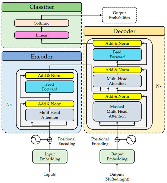
Figure 1. Overall architecture of Transformer.

2.1.1. Embeddings and Positional Encoding

In natural language processing, embedding techniques facilitate data processing through the transformation of high-dimensional sparse word vectors into low-dimensional dense vectors. We employ an analogous methodology to handle sequence data, projecting the input data into a low-dimensional space through an embedding layer [82]. To capture the sequential information within a time series, we incorporate positional encoding, leveraging sine and cosine functions with varying frequencies to denote positional information. More precisely, the positional encoding comprises a combination of sine and cosine functions, as depicted in Equations (1) and (2).

$$PE\left(t,2s\right)=sin\left({\displaystyle \frac{t}{{10000}^{2s/d}}}\right)$$

(1)

$$PE\left(t,2s+1\right)=cos\left({\displaystyle \frac{t}{{10000}^{2s/d}}}\right)$$

(2)

where s denotes the dimension of positional encoding, while d represents the dimension of set transformation, satisfying $1\le 2s\le d$. Following the incorporation of positional encoding information $PE\in R^{T\times d}$ into the embedded input, the combined data is fed into the encoder layer to undergo further processing.

2.1.2. Encoder–Decoder Module

The Transformer architecture builds its encoder and decoder modules by stacking multiple layers with identical structures. Each encoder layer contains two sublayers: multi-head self-attention and a fully connected feedforward neural network. Both sublayers use residual connections and layer normalization, which help the model converge faster and reduce the risk of overfitting. The decoder has a similar structure but adds a masked multi-head self-attention sublayer to its self-attention component. This masking ensures that, when predicting the current output, the decoder only uses previously generated outputs. This prevents information leakage and improves the model’s prediction accuracy. The self-attention mechanism extracts key information from sequential data, allowing the model to better understand dependencies within the sequence. The output of the i-th self-attention mechanism is defined as follows [70]:

$$Attentio{n}_i\left(Q_i,K_i,V_i\right)=Softmax\left({\displaystyle \frac{Q_i\cdot K_i^T}{\sqrt{d}}}\right)\cdot V_i$$

(3)

where $d_k$ denotes the dimension of the linear projection matrix, while $Softmax$ represents the activation function. The computations of $Q_i$, $K_i$, and $V_i$, as shown in Equation (4), indicate the query (Q), key (K), and value (V) matrices initialized from the input feature samples X through linear projection matrices $W^Q$, $W^K$, and $W^V$, respectively.

$$\left\{\begin{array}{l}{Q}_i=X\cdot W_i^Q\\ K_i=X\cdot W_i^K\\ V_i=X\cdot W_i^V\end{array}\right.$$

(4)

The multi-head self-attention mechanism is a cornerstone component of the Transformer model. As shown in Figure 2, it is composed of a self-attention layer, a concatenation layer, and a linear transformation layer.

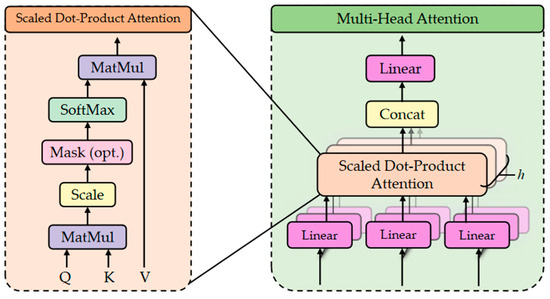
Figure 2. Schematic diagram of multi-head attention mechanism.

This mechanism, by integrating multiple independently parameterized self-attention networks, is capable of capturing dependencies from diverse perspectives. Consequently, it more accurately characterizes the temporal and spatial features of the data compared to conventional attention mechanisms. Within the multi-head self-attention mechanism, each attention function operates in parallel with its corresponding projected versions of the query, key, and value matrices. Subsequently, the outputs of all attention functions are aggregated through a linear layer to generate the final output. The computational formula for the multi-head self-attention mechanism is as follows:

$$\mathrm{M}\mathrm{u}\mathrm{l}\mathrm{t}\mathrm{i}\mathrm{H}\mathrm{e}\mathrm{a}\mathrm{d}\left(Q,K,V\right)=Concat\left(Attentio{n}_1,Attentio{n}_2,...,Attentio{n}_h\right)W^o$$

(5)

where $W^O$ denotes the weights of the corresponding network, while $h$ indicates the number of heads.

2.1.3. Classifier

The data processed by the encoder–decoder architecture is first subjected to output mapping through a linear layer to transform it into an appropriate dimensional space. Subsequently, the output values are normalized into probabilities within the range of 0 to 1 using the softmax function. Finally, the class with the highest probability is selected as the classification outcome.

2.2. Newton–Raphson-Based Optimizer

The NRBO is an advanced metaheuristic optimization algorithm proposed by Sowmya et al. in 2024 [83]. Building upon the classical Newton–Raphson method (NRM), the NRBO innovatively integrates the Newton–Raphson search rule (NRSR) and the trap avoidance operator (TAO), thereby significantly enhancing its exploration capability and convergence rate. In particular, the introduction of the TAO effectively mitigates the interference of local optimum traps, ensuring the global stability of the optimization process. In practical applications, the NRBO not only demonstrates strong global search capabilities but also significantly improves the generalization and accuracy of models when dealing with complex optimization problems, providing robust support for efficient hyperparameter optimization.

The NRM is a process of finding function roots by utilizing the leading components of the Taylor series (TS) to locate roots near the assumed root [84]. Starting from an initial point $x_0$, NRM uses the TS evaluated at $x_0$ to identify another point near the previous solution. This step is repeated until the correct solution is found. The second-order Taylor series expansion for point $x=x_0+\delta$ is expressed as follows:

$$\mathrm{g}\left(x_0+\delta \right)\approx g^{\prime }\left(x_0\right)\delta +{\displaystyle \frac{g^{\prime \prime }\left(x_0\right){\left(\delta \right)}^2}{2}}$$

(6)

Based on Equation (6), the displacement $\delta ={\delta }_0$ required to search for a root closer to $x_0$ is illustrated as follows:

$${\delta }_0=-{\displaystyle \frac{g^{\prime }\left(x_0\right)}{g^{\prime \prime }\left(x_0\right)}}$$

(7)

By iteratively repeating Equation (8) until convergence, the optimal root is achieved.

$$y_{m+1}=y_m+{\delta }_m$$

(8)

Although the algorithm may become unbalanced near local maxima or horizontal asymptotes, an appropriate initial position enables the iterative identification of the next approximation. The algorithm employs the NRM to identify the search region and leverages multiple vector sets, as well as the NRSR and TAO operators, to define the search path for exploring the search region. The specific implementation steps of the algorithm are divided into three parts: population initialization, the Newton–Raphson search rule, and the trap avoidance operation.

2.2.1. Population Initialization

The NRBO algorithm initiates the search for the optimal solution by generating an initial random population within the boundaries of candidate solutions. Given the presence of $N_p$ populations, each composed of fuzzy decision vectors, the random population is generated using Equation (9).

$$x_j^n=lb+rand·\left(ub-lb\right),n=\mathrm{1,2},...,N_{p}andj=\mathrm{1,2},...,dim$$

(9)

where $x_j^n$ indicates the position of the j-th dimension of the n-th population, while $rand$ denotes a random number between 0 and 1. The population matrix, which delineates all dimensions of the population, is presented in Equation (10).

$$X_n={\left[\begin{array}{cc}\begin{array}{c}{x}_2^1\\ x_1^2\end{array}& \begin{array}{cc}\begin{array}{c}{x}_2^1\\ x_2^2\end{array}& \begin{array}{cc}\begin{array}{c}\dots \\ \dots \end{array}& \begin{array}{c}{x}_{dim}^1\\ x_{dim}^2\end{array}\end{array}\end{array}\\ \begin{array}{c}⋮\\ x_1^{N_p}\end{array}& \begin{array}{cc}\begin{array}{c}⋮\\ x_2^{N_p}\end{array}& \begin{array}{cc}\begin{array}{c}\ddots \\ \dots \end{array}& \begin{array}{c}⋮\\ x_{dim}^{N_p}\end{array}\end{array}\end{array}\end{array}\right]}_{N_{p\times dim}}$$

(10)

2.2.2. Newton–Raphson Search Rule

During the optimization process, vectors are controlled by the NRSR, enabling the population to explore the feasible region more accurately and acquire superior positions. To derive the NRSR, it is necessary to employ Taylor expansion to determine the second-order derivative. The Taylor series expansions of $g\left(x-∆x\right)$ and $g\left(x+∆x\right)$ are presented as follows:

$$g\left(x+\mathsf{\Delta }x\right)=g\left(x\right)+g^{\prime }\left(x_0\right)\mathsf{\Delta }x+{\displaystyle \frac{1}{2!}}{g}^{\prime \prime }\left(x_0\right)\mathsf{\Delta }{x}^2+{\displaystyle \frac{1}{3!}}{g}^{\prime \prime \prime }\left(x_0\right)\mathsf{\Delta }{x}^3+...$$

(11)

$$\begin{array}{l}g\left(x-\mathsf{\Delta }x\right)=g\left(x\right)-g^{\prime }\left(x_0\right)\mathsf{\Delta }x+{\displaystyle \frac{1}{2!}}{g}^{\prime \prime }\left(x_0\right)\mathsf{\Delta }{x}^2-{\displaystyle \frac{1}{3!}}{g}^{\prime \prime \prime }\left(x_0\right)\mathsf{\Delta }{x}^3+...\end{array}$$

(12)

Combining Equations (7), (11) and (12), we can derive the updated root locations of the NRSR as shown in Equation (13).

$$x_{n+1}=x_n-{\displaystyle \frac{\left(g\left(x_n+\mathsf{\Delta }x\right)-g\left(x_n-\mathsf{\Delta }x\right)\right)\cdot \mathsf{\Delta }x}{2\cdot \left(g\left(x_n+\mathsf{\Delta }x\right)+g\left(x_n-\mathsf{\Delta }x\right)-2\cdot x_n\right)}}$$

(13)

The adjacent positions $x_n$ are denoted as $x_n+∆x$ and $x_n+∆x$, and the NRSR expression is as follows:

$$NRSR=randn\times {\displaystyle \frac{\left(X_w-X_b\right)\cdot \mathsf{\Delta }x}{2\times \left(X_w+X_b-2\cdot x_n\right)}}$$

(14)

In the NRBO algorithm, Equation (14) incorporates stochastic parameters, where $rand$ denotes normally distributed random numbers with a mean of zero and a variance of one, $X_w$ indicates the worst position, and $X_b$ represents the best position. By leveraging the current solution to assist in position updates, Equation (14) enhances the quality of the current solution. This design not only improves the NRBO’s search ability but also better balances exploitation and exploration. The expression for $∆x$ is shown in Equation (15).

$$\begin{array}{c}\mathsf{\Delta }x=rand\left(1,\mathrm{d}\mathrm{i}\mathrm{m}\right)\times \left|X_b-X_n^{IT}\right|\end{array}$$

(15)

where $X_b$ denotes the best solution obtained thus far, while $rand(1,dim)$ represents random numbers with dim-dimensional decision variables. Based on empirical evidence, optimization algorithms need to strike a balance between diversity and convergence to detect optimal solutions in the search space and ultimately converge to global solutions. To this end, an adaptive coefficient $\delta$ can be introduced to enhance the algorithm’s performance. The expression for $\mathsf{\delta }$ is shown in Equation (16).

$$\delta ={\left(1-\left({\displaystyle \frac{2\times IT}{Ma{x}_{I}T}}\right)\right)}^5$$

(16)

where $IT$ denotes the current iteration count, while $Max\_IT$ represents the maximum number of iterations. During the iteration process, $\delta$ self-adapts to balance the exploration and exploitation phases, significantly cutting down the number of iterations. By factoring in the stochastic behavior during optimization, it boosts diversity and averts local optima, thereby enhancing the NRBO algorithm.

Subsequently, to further enhance the utilization efficiency of the NRBO algorithm, another parameter $\rho$ is introduced. This parameter steers the population toward the correct direction, thereby optimizing the search process. The expression for $\rho$ is shown in Equation (17).

$$\rho =ran{d}_1\times \left(X_b-X_n^{IT}\right)+ran{d}_2\times \left(X_{r_1}^{IT}-X_{r_2}^{IT}\right)$$

(17)

where $rand$ denotes random numbers in (0, 1), $r_1$ and $r_2$ represent distinct integers randomly selected from the population, and the current position of the vector $X_n^{\prime IT}$ is updated via Equation (18).

$$X_n^{\prime IT}=x_n^{IT}-\left(randn\times {\displaystyle \frac{\left(X_w-X_b\right)\times \mathsf{\Delta }x}{2\times \left(X_w+X_b-2\times X_n\right)}}\right)+\rho$$

(18)

Building on the NRM framework, the NRSR has been further optimized, and Equation (14) has been accordingly rewritten to yield Equation (19).

$$NRSR=randn\times {\displaystyle \frac{\left({\mathrm{y}}_w-y_b\right)\cdot \mathsf{\Delta }x}{2\times \left(y_w+y_b-2\cdot x_n\right)}}$$

(19)

$$y_w=rand\times \left(Mean\left(Z_{n+1}+x_n\right)+r_1\times ∆x\right)$$

(20)

$$y_b=rand\times \left(Mean\left(Z_{n+1}+x_n\right)-r_1\times ∆x\right)$$

(21)

$$Z_{n+1}=x_n-randn\times {\displaystyle \frac{\left(X_w-X_b\right)\times ∆x}{2\times \left(X_w+X_b-2\times x_n\right)}}$$

(22)

where $y_w$ and $y_b$ denote the positions of two vectors generated by $Z_{n+1}$ and $x_n$, respectively, with the enhanced version of the NRSR presented in Equation (19). Subsequent to applying Equation (19), Equation (18) is accordingly updated to Equation (23), as detailed below.

$$X_n^{\prime IT}=x_n^{IT}-\left(randn\times {\displaystyle \frac{\left(y_w-y_b\right)\times \mathsf{\Delta }x}{2\times \left(y_w+y_b-2\times x_n\right)}}\right)+\rho$$

(23)

To better guide the population’s search direction, it is necessary to replace the position of the optimal vector $X_b$ with that of the current vector $X_n^{\prime IT}$ as shown in Equation (23), thereby constructing a novel vector $X_n^{\prime \prime IT}$, which is presented in Equation (24).

$$X_n^{\prime \prime IT}=X_{\mathrm{b}}-\left(randn\times {\displaystyle \frac{\left(y_w-y_b\right)\times \mathsf{\Delta }x}{2\times \left(y_w+y_b-2\times x_n\right)}}\right)+\rho$$

(24)

In the development phase of the NRBO algorithm, the search direction strategy primarily focuses on balancing local and global search capabilities. Specifically, Equation (25) is effective for local search but has limitations in global search. Conversely, Equation (24) is advantageous for global search but less effective for local search. To overcome these limitations, the NRBO algorithm employs both Equations (24) and (25). This combined approach enhances diversity and strengthens the exploitation phase. The new position vector is updated via Equations (25) and (26).

$$x_n^{IT+1}=ran{d}_1\times \left(ran{d}_1\times X_n^{\prime T}+\left(1-ran{d}_1\right)\times X_n^{\prime \prime IT}\right)+\left(1-ran{d}_1\right)\times X_n^{\prime \prime IT}$$

(25)

$$X_n^{\prime \prime \prime IT}=X_n^{IT}-\delta \times \left(X_n^{\prime \prime IT}-X_n^{\prime IT}\right)$$

(26)

2.2.3. Trap Avoidance Operation

To enhance the NRBO algorithm’s ability to solve practical problems, the TAO is incorporated. The TAO combines the best position $X_b$ with the current vector position $X_{IT}^n$ to generate superior solutions $X_{IT}^{TAO}$. When the random number $\mathrm{r}\mathrm{a}\mathrm{n}\mathrm{d}$ is below the threshold $\mathrm{D}\mathrm{F}$, $X_{IT}^{TAO}$ is generated according to Equation (27).

$$\left\{\begin{array}{c}{X}_{IT}^{TAO}=X_n^{IT+1}+{\theta }_1\left({\mu }_1·x_b-{\mu }_2·X_n^{IT}\right)+{\theta }_1·\delta \left({\mu }_1·Mean\left(X^{IT}\right)-{\mu }_2·X_n^{IT}\right),if{\mu }_1<0.5\\ X_{IT}^{TAO}=x_b+{\theta }_1\left({\mu }_1·x_b-{\mu }_2·X_n^{IT}\right)+{\theta }_1·\delta \left({\mu }_1·Mean\left(X^{IT}\right)-{\mu }_2·X_n^{IT}\right),otherwise\end{array}\right.$$

(27)

where ${\theta }_1$ and ${\theta }_2$ are uniformly distributed random numbers within the ranges of (−1, 1) and (−0.5, 0.5), respectively. $\mathrm{D}\mathrm{F}$ is a critical factor influencing the performance of the NRBO algorithm. $\mu 1$ and $\mu 2$ are also random numbers determined by the binary variable $\beta$ (which takes a value of 0 or 1) and are calculated via Equations (28) and (29), respectively.

$${\mu }_1=\beta \times 3\times rand+\left(1-\beta \right)$$

(28)

$${\mu }_2=\beta \times rand+\left(1-\beta \right)$$

(29)

The NRBO algorithm, leveraging its distinctive random search and adaptive adjustment mechanisms, can efficiently explore and exploit hyperparameter search spaces. Its stochastic nature ensures population diversity, effectively avoiding local optimum traps and enhancing its search optimization capabilities. This diverse search strategy is critical for complex tasks like wind speed forecasting. It ensures models excel locally, converge faster, and optimize globally across the entire parameter space. Consequently, the NRBO offers a powerful hyperparameter optimization method for Transformer models in wind speed forecasting, significantly improving prediction accuracy and model generalization. Figure 3 illustrates the specific process of optimizing Transformer model hyperparameters using the NRBO algorithm.

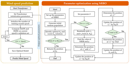
Figure 3. The specific process of optimizing Transformer model hyperparameters through the NRBO algorithm.

2.3. XGBoost

The gradient-boosted decision tree (GBDT) algorithm, proposed by Friedman in 2001 [85], iteratively constructs new trees via gradient descent to minimize the objective function. Each new tree is built upon the foundation of all previous ones [86]. The ensemble model of trees is presented in Equation (30).

$${\widehat{y}}_i=\sum _{k=1}^K{f}_k\left(x_i\right),f_k\in F$$

(30)

where ${\widehat{y}}_{\mathrm{i}}$ denotes the expected value of the i-th sample, and $x_i$ specifies the i-th data point of the input feature vector. Based on this concept, Chen et al. proposed a more advanced algorithm called Extreme Gradient Boosting (XGBoost) [87]. It is an ensemble method based on decision trees and is suitable for both classification and regression tasks. In regression, XGBoost builds new trees sequentially, using each new classification and regression tree (CART) to fit the residuals of the previous model [88,89]. Compared to GBDT, XGBoost offers two major advantages: it supports parallel computation during boosting and handles complex datasets more effectively. In this study, we use the XGBoost algorithm to correct residual errors, thereby improving prediction accuracy. The objective function of XGBoost typically comprises a loss function $L_{loss}$ and a regularization term $\Omega \left(f_k\right)$, as shown below.

$$L_{loss}=\sum _{i=1}^k\phi \left(y_i,{\widehat{y}}_i\right)+\sum _{k=1}^k\mathsf{\Omega }\left(f_k\right)$$

(31)

$$\mathsf{\Omega }\left(f\right)=\gamma T+{\displaystyle \frac{1}{2}}\lambda {\parallel w\parallel }^2$$

(32)

where $T$ denotes the number of leaves; $\gamma$ and $\lambda$ are penalty coefficients; and $\mathrm{w}$ represents the score vector on the leaves. To minimize the loss function as much as possible, an incremental function is introduced at each iteration, as shown in Equation (33).

$$L_{loss}^{\left(t\right)}=\sum _{i=1}^n\phi \left(y_i,{\widehat{y}}_i^{\left(t-1\right)}+f_t\left(x_i\right)\right)+\mathsf{\Omega }\left(f_t\right)$$

(33)

To conduct a second-order Taylor expansion of the aforementioned equation, we can derive the following formula:

$$\left\{\begin{array}{l}{g}_i={\partial }_{\widehat{y}\left(t-1\right)}L\left(y_i,{\widehat{y}}_i^{\left(t-1\right)}\right)\\ h_i={\partial }_{\widehat{y}\left(t-1\right)}^{2}L\left(y_i,{\widehat{y}}_i^{\left(t-1\right)}\right)\end{array}\right.$$

(34)

$$L_{loss}^{\left(t\right)}=\sum _{i=1}^T\left[G_i{w}_j+{\displaystyle \frac{1}{2}}\left(H_j+\lambda w_j^2\right)\right]+\gamma T$$

(35)

Among them, $G_j={\sum }_{i\in I_j}{g}_j$, $H_j={\sum }_{i\in I_j}{h}_j$, and $w_j$ are mutually independent variables. Subsequently, we reformulate Equation (16) into a single-variable quadratic function in terms of ${\mathrm{w}}_{\mathrm{j}}$, yielding an optimal solution for ${\mathrm{w}}_{\mathrm{j}}$ denoted as $-{\displaystyle \frac{G_j}{H_j+\lambda }}$. Upon substituting this solution back into Equation (16), we derive the final objective function.

$$L_{loss}^{\left(t\right)}=-\sum _{i=1}^T{\displaystyle \frac{G_j^2}{H_j+\lambda }}+\lambda T$$

(36)

Figure 4 provides a detailed illustration of the mechanism by which the XGBoost algorithm operates when applied to wind speed forecasting tasks.

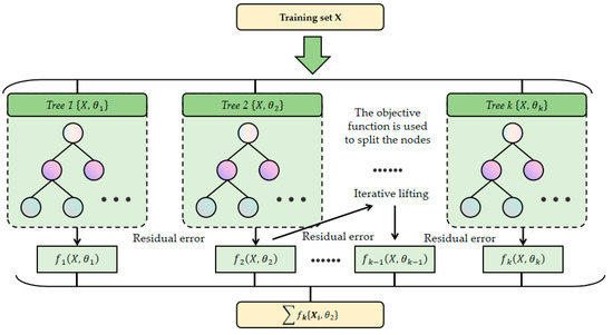
Figure 4. Schematic diagram of XGBoost model.

2.4. Framework of the NRBO-TXAD Model

The NRBO-TXAD model integrates data preprocessing, model optimization, and error compensation into a unified framework for wind speed prediction. The architecture consists of three core modules: a data preprocessing module, a Transformer-based prediction module optimized by the NRBO, and an XGBoost-based error compensation module. These modules work together to form a closed-loop prediction system. The structure is summarized in Table 5.

Table 5. Overview of NRBO-TXAD model architecture.

Module	Key Methods	Function
Data preprocessing	IQR method, adaptive moving average filter	Removes outliers, smooths the series, and ensures high-quality input
Transformer prediction	NRBO optimization, self-attention mechanism	Extracts temporal features and provides initial predictions
Error compensation	XGBoost residual modeling	Learns residual patterns and improves prediction accuracy

The model first applies the IQR method to eliminate outliers. Then, it uses an adaptive moving average filter to smooth the time series data while preserving important features. The preprocessed data is input into a Transformer network whose key hyperparameters (learning rate, number of attention heads, L2 regularization coefficient) are optimized by the NRBO algorithm. This module captures both short-term and long-term dependencies and outputs an initial prediction. The XGBoost module then takes the residuals from the Transformer and models their nonlinear patterns to generate correction values. These values are combined with the initial predictions to produce the final wind speed forecast.

The three modules are closely linked. High-quality data supports accurate modeling, parameter optimization enhances learning efficiency, and residual compensation reduces systematic errors. Together, they form a robust and precise prediction framework. In order to verify the effectiveness of this model, the overall process of this study is illustrated in Figure 5.

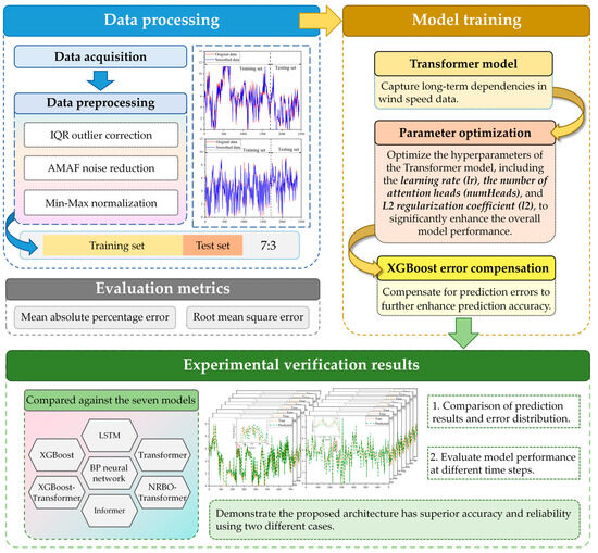
Figure 5. Framework of proposed methodology.

3. Case Study Analysis

3.1. Dataset Description and Preprocessing

To systematically evaluate the generalization ability and forecasting performance of our proposed model, we selected two wind speed datasets with distinct time spans and sampling frequencies for comparative analysis. Dataset 1 originates from a wind farm, with a 10 min sampling interval from 14 March 2022, to 30 March 2022 (16 days), comprising 2448 sampling points. We addressed missing values using cubic spline interpolation, a method referenced from the literature [90]. In contrast, Dataset 2 features 2390 wind speed data points without missing values, sampled hourly from 3 June 2020 (20:00) to 11 September 2020 (09:00), spanning 3 months. The training and testing datasets were split in a 7:3 ratio, with default three-step-ahead predictions. The prediction experiments were based on the average results of ten independent trials.

Wind speed data, typically sourced from weather stations, wind turbines, or other sensors, is often compromised by environmental factors, equipment malfunctions, or human operations, leading to noisy data with outliers and anomalies. To enhance data quality and model robustness, we employed two data preprocessing techniques: the IQR method for outlier removal and an innovative AMAF for noise reduction and data smoothing.

3.1.1. IQR Outlier Detection and Correction

To calculate the IQR, we use the upper and lower quartiles of the dataset. Let ${\mathcal{Q}}_1$ represent the 25th percentile (lower quartile) and ${\mathcal{Q}}_3$ represent the 75th percentile (upper quartile). The IQR is defined as the difference between these two quartiles.

$$IQR=Q_3-Q_1$$

(37)

To define the lower and upper bounds, we use 1.5 times the IQR as the threshold. Any wind speed values beyond this range are regarded as outliers and truncated at the corresponding upper or lower boundary values, as follows:

$$x_i=\left\{\begin{array}{l}{Q}_1-1.5\cdot IQR,x_i>Q_1-1.5\cdot IQR\\ x_i,Q_1-1.5\cdot IQR\le x_i\le Q_3+1.5\cdot IQR\\ Q_3+1.5\cdot IQR,x_i>Q_3+1.5\cdot IQR\end{array}\right.$$

(38)

3.1.2. Adaptive Moving Average Filter

Traditional sliding window methods have a fixed window length, which fails to adapt to local fluctuation features. To address this, we introduce an adaptive sliding window strategy. Using the minimum MSE criterion, it can adaptively select the optimal window width within a preset window range.

$$MSE\left(w\right)={\displaystyle \frac{1}{N}}\sum _{i=1}^N{\left(x_i-{\widehat{x}}_i^{\left(w\right)}\right)}^2$$

(39)

where ${\widehat{x}}_i^{\left(w\right)}$ represents the smoothed estimate for the i-th point when the window width is $w$. We ultimately select the $w^{*}$ that minimizes the MSE as the optimal window size. In this paper, we set $w_{min}$ to 3 and $w_{max}$ to 9.

$$w^{*}=arg\underset{w\in \left[w_{min},w_{max}\right]}{min}MSE\left(w\right)$$

(40)

The proposed AMAF treats consecutively sampled data as a queue of optimal length ${\omega }^{*}$. After a new measurement, the first piece of data in the queue is deleted, the remaining $({\omega }^{*}-1)$ data move forward, and the new data is inserted at the end. Finally, Equation (41) is used to obtain $y\left(z\right)$ as the output [91].

$$y\left(z\right)={\displaystyle \frac{x\left(z\right)+x\left(z-1\right)+x\left(z-2\right)\dots x\left(z-{\omega }^{*}+1\right)}{{\omega }^{*}}}$$

(41)

The data, after being processed, undergoes Min–max normalization as shown in Equation (41). This ensures that input features lie within the [0, 1] interval, enhancing the neural network’s training convergence speed and stability.

$$x_i^{\prime }={\displaystyle \frac{x_i-x_{min}}{x_{max}-x_{min}}}$$

(42)

As shown in Table 6 and Figure 6, the statistical metrics of the data before and after processing indicate that the mean and standard deviation decreased slightly, while skewness and kurtosis moved closer to a normal distribution. For Case 1’s dataset, the IQR method effectively curbed high-end outliers, reducing the maximum value from 14.03 to 11.28 m/s. It also decreased skewness from 0.4403 to 0.2205 and kurtosis from 3.40 to 2.91, indicating a more symmetric and near-normal data distribution. The AMAF was then applied for noise reduction. It kept the mean (5.3994) and median (5.3500) nearly unchanged but further lowered the standard deviation from 2.6305 to 2.5905, easing local fluctuations and making the wind speed sequence smoother. This helps the model learn time-dependent features more stably. For Case 2’s dataset, the data quality was already high, so the IQR method caused almost no changes. After AMAF processing, the standard deviation slightly decreased from 1.7975 to 1.7643, with minimal values rising slightly (0.02 to 0.06 m/s) and maximum values dropping slightly (9.16 to 8.83 m/s), showing a mild suppression of extremes by the filter. Notably, in the adaptive window search for both datasets, a window size of 3 was selected. This suggests that local smoothing can significantly enhance data quality while avoiding information loss from over-filtering.

Table 6. Data statistics before and after processing.

Dataset	Processing Method	Mean	Median	Std	Skewness	Kurtosis	Min	Max	Optimal Window
Case 1	Raw	5.4455	5.3500	2.7438	0.4403	3.3986	0.0200	14.0300	-
	IQR	5.3994	5.3500	2.6305	0.2205	2.9122	0.0200	11.2762	-
	AMAF	5.3994	5.3500	2.5905	0.2451	2.9376	0.0200	11.2762	3
Case 2	Raw	4.5150	4.7000	1.7975	−0.2607	2.7650	0.0200	9.1600	-
	IQR	4.5150	4.7000	1.7975	−0.2607	2.7650	0.0200	9.1600	-
	AMAF	4.5149	4.6983	1.7643	−0.2512	2.7510	0.0600	8.8300	3

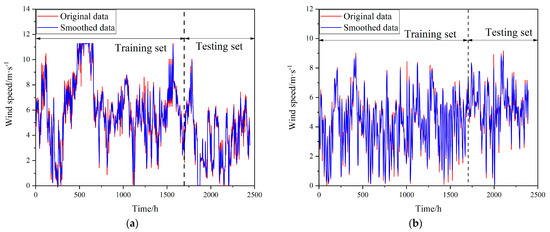
Figure 6. Visualization of data before and after processing: (a) Case 1; (b) Case 2.

Figure 7 and Figure 8 demonstrate the wind speed probability distribution for the two cases, respectively presenting the original and smoothed data. By comparison, the impact of smoothing on the wind speed probability distribution becomes evident.

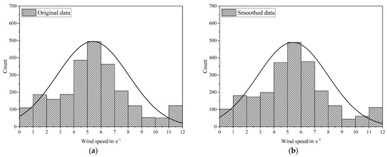
Figure 7. Wind speed probability distribution for Case 1: (a) raw data; (b) smoothed data.

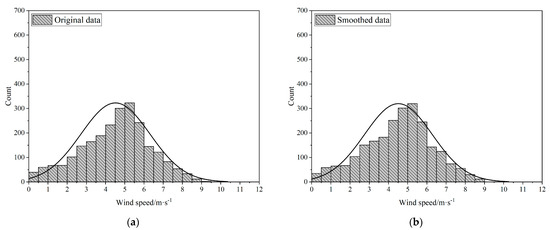
Figure 8. Wind speed probability distribution for Case 2: (a) raw data; (b) smoothed data.

3.2. Evaluation Metrics

We use the MAPE and RMSE to evaluate the prediction model’s performance. MAPE measures the average of the absolute percentage errors between predicted and actual values, calculated as shown in Equation (43).

$${\delta }_{\mathrm{M}\mathrm{A}\mathrm{P}\mathrm{E}}={\displaystyle \frac{1}{\mathrm{n}}}\sum _{\mathrm{i}=1}^n\left|{\displaystyle \frac{y_i-{\widehat{y}}_i}{y_i}}\right|\times 100\mathrm{\%}$$

(43)

Here, $y_i$ indicates the actual value of the i-th sample, $\widehat{y}$ represents the predicted value of the i-th sample, and $n$ is the total number of samples. The MAPE offers a clear percentage-based measure of prediction error, which facilitates easy comparison across models. It is particularly useful for evaluating proportional errors. However, the MAPE can become unstable when the actual values are close to zero. To address this issue, we also use the RMSE, which is calculated as the square root of the average squared differences between predicted and actual values, as shown in Equation (44).

$${\delta }_{\mathrm{R}\mathrm{M}\mathrm{S}\mathrm{E}}=\sqrt{{\displaystyle \frac{1}{\mathrm{n}}}\sum _{i=1}^n{\left(y_i-{\widehat{y}}_i\right)}^2}$$

(44)

3.3. Simulation Environment

All simulation experiments were conducted on a personal laptop with Matlab R2024a. The laptop was configured with a 2.40-GHz 11th Gen Intel Core i5-1135G7 processor, Intel Iris Xe graphics, and 16 GB of RAM (Intel, Santa Clara, CA, USA).

4. Experimental Results

4.1. Parameter Setting and Comparison Model

We conducted comparative experiments of the proposed method with seven mainstream wind speed forecasting baseline models, as shown in Table 7.

Table 7. Description of each model.

Model Name	Model Description
BP neural network [92]	A feedforward neural network trained through backpropagation, capable of learning complex nonlinear relationships between inputs and outputs.
XGBoost [93]	An ensemble learning algorithm based on gradient boosting that combines multiple weak learners to improve predictive performance.
Transformer [94]	Utilizes a self-attention mechanism to capture long-range dependencies in sequential data.
Informer [95]	Employs the ProbSparse self-attention mechanism and self-attention distillation to reduce computational complexity.
LSTM [96]	A special type of recurrent neural network that uses gating mechanisms to effectively address the vanishing gradient problem in traditional RNNs.
NRBO–Transformer	Combines the Transformer model with the NRBO optimization algorithm, optimizing network structure and parameters to further enhance long sequence processing capabilities.
XGBoost–Transformer	Combines the error compensation value predicted by the XGBoost model with the predicted values from the Transformer model to obtain the final wind speed forecasting results.

All models were optimized using the Adam optimizer. Additionally, the parameters for each model were set as shown in Table 8.

Table 8. Hyperparameter settings for each model.

Model	Hyperparameter Settings
BP neural network	Hidden layer nodes: 11; initial learning rate: 0.001; epochs: 100; min_grad: 1 × 10−6.
XGBoost	Estimators: 600; maximum depth: 4; minimum child weight: 1; initial learning rate: 0.002; epochs: 100.
Transformer	Heads: 8; dimension (dm): 128; hidden neurons: 64; dropout rate: 0.1; initial learning rate: 0.001; epochs: 100; encoder–decoders: 1.
Informer	Heads: 4; dimension (dm): 128; hidden neurons: 128; dropout rate: 0.1; initial learning rate: 0.002; epochs: 100; encoder–decoders: 2.
LSTM	Hidden size: 128; number of layers: 2; dropout rate: 0.1; initial learning rate: 0.002; epochs: 100.
NRBO–Transformer	Heads, L2 regularization, learning rate: to be optimized; for other settings, refer to Transformer.
XGBoost–Transformer	Refer to the settings of XGBoost and Transformer.

In this study, the NRBO optimizes three hyperparameters of the Transformer model, namely the learning rate (lr), the number of attention heads (numHeads), and the L2 regularization coefficient (l2). The respective ranges for these parameters are set as follows: the range of lr is [1 × 10⁻³, 1 × 10⁻²], the range of numHeads is [2, 8], and the range of l2 is [1 × 10⁻⁴, 1 × 10⁻¹]. Additionally, the population size for NRBO is set to 5, with a maximum of 20 iterations.

During the actual training process, the sliding window technique is employed. This technique reconstructs the input–output relationship by transforming univariate data into a supervised learning format. Specifically, the model generates an output window that is aligned with the input time steps immediately after receiving the corresponding input window [97]. As it moves forward, the oldest set of time steps is discarded each time to avoid data leakage [98], thereby ensuring more robust and efficient training, which is shown in Figure 9.

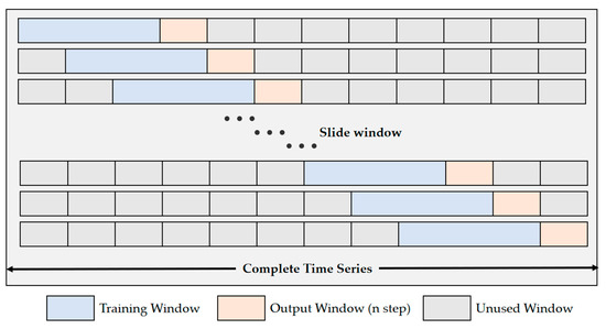
Figure 9. Schematic diagram of the sliding window for time series forecasting.

4.2. Fitness Curve

The iteration curve of the NRBO algorithm is shown in Figure 10. For Case 1, the algorithm approaches the convergence value after the sixth iteration, with the fitness value stabilizing at 0.7307. For Case 2, the algorithm approaches the convergence value after the 3rd iteration and reaches convergence at the 10th iteration, with the fitness value stabilizing around 0.3030. The hyperparameter optimization results for the two different wind speed datasets are shown in Table 9.

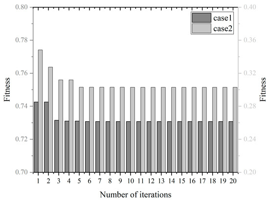
Figure 10. Iteration curve of NRBO algorithm.

Table 9. Parameter optimization of proposed model.

Case	Parameters	Quantity
Case 1	lr	0.00578
	numHeads	8
	l2	0.0001002
Case 2	lr	0.00629
	numHeads	3
	l2	0.0001000

4.3. Prediction and Error Plots

In this study, we selected the BP, XGBoost, Transformer, Informer, and LSTM models as the comparison models for single models and chose NRBO–Transformer and XGBoost–Transformer as the comparison models for hybrid models. Figure 11 and Figure 12 show the prediction results of different models for different cases. Among them, the prediction curve of the proposed model in this paper is the closest to the true value. In addition, the enlarged views in both sets of figures show the peak-capturing plots of different models, from which it can be seen that the proposed model in this paper has the ability to capture strong volatility and nonlinearity of peaks. Moreover, both the degree of approaching the true value by adding the NRBO for hyperparameter optimization and by adding XGBoost for error compensation exceed that of single models, indicating a synergistic effect between them.

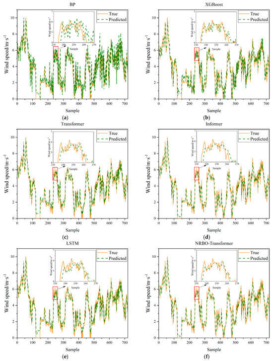
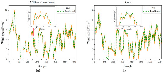
Figure 11. Visualization of prediction curves of eight models in Case 1: (a) BP; (b) XGBoost; (c) Transformer; (d) Informer; (e) LSTM; (f) NRBO-Transformer; (g) XGBoost-Transformer; (h) Ours.

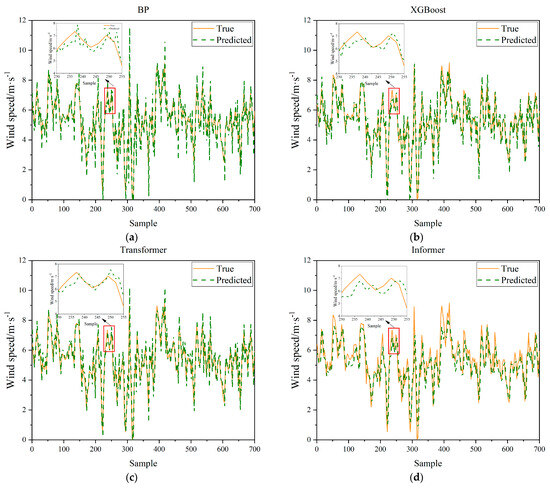
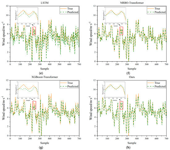
Figure 12. Visualization of prediction curves of eight models in Case 2: (a) BP; (b) XGBoost; (c) Transformer; (d) Informer; (e) LSTM; (f) NRBO-Transformer; (g) XGBoost-Transformer; (h) Ours.

For Case 1 (Figure 11), the prediction curve of the BP neural network model is relatively smooth overall but deviates significantly from the true values in regions of sharp fluctuations. The XGBoost model performs well in capturing upward trends but still exhibits noticeable errors around the peaks. The Transformer model can follow the overall trend of the true values reasonably well but lacks precision in fitting the detailed fluctuations. The Informer model excels in grasping the overall trend but is somewhat insufficient at capturing local variations. The LSTM model has certain advantages in predicting time series data but still has errors when dealing with complex fluctuations. The hybrid models, NRBO–Transformer and XGBoost–Transformer, show relatively better performance but still have deviations. In contrast, the proposed model in this paper (NRBO-TXAD) has a prediction curve that is the closest to the true values. It not only maintains high consistency in the overall trend but also captures the changes in the true values well in detailed fluctuations, demonstrating an excellent ability to capture strong volatility and nonlinear peaks.

In Case 2 (Figure 12), the performance of the models also follows a similar pattern. By comparing the prediction curves of the two cases, it can be observed that the proposed model in this paper demonstrates good adaptability and superiority in different scenarios, effectively improving the accuracy and reliability of predictions.

Figure 13 and Figure 14 illustrate the error distributions of different models for Case 1 and Case 2, respectively. By comparing the error plots, the differences in prediction stability and accuracy among the models can be clearly observed. For Case 1 (Figure 13), the error distributions of the BP, XGBoost, and Transformer models exhibit significant dispersion, indicating a higher number of large deviation points in wind speed prediction. In particular, the BP model has the widest error range, which signifies its weakest prediction capability.

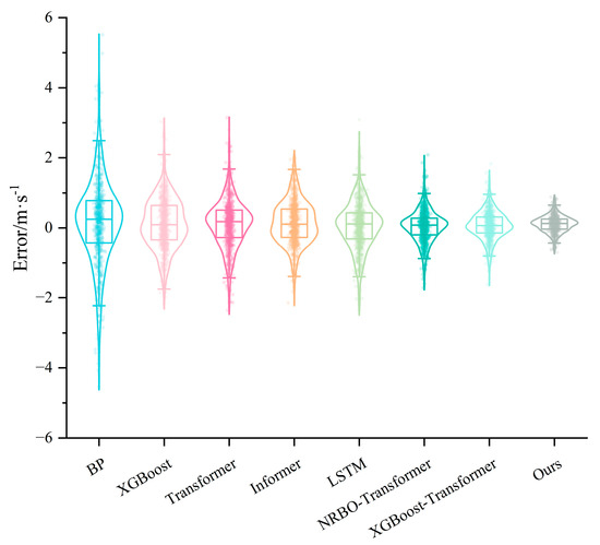
Figure 13. The violin plot of prediction error for Case 1.

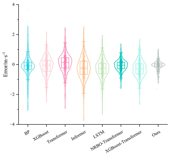
Figure 14. The violin plot of prediction error for Case 2.

For Case 2 (Figure 14), the error distributions of the BP, Transformer, Informer, and LSTM models exhibit significant dispersion, with the Informer model having the widest error range. This reflects its insufficient adaptability to complex wind speed sequences. In contrast, the hybrid models incorporating optimization mechanisms and the Transformer architecture, namely XGBoost–Transformer and NRBO–Transformer, show more concentrated error distributions. The proposed model in this study (NRBO-TXAD) has the most compact error distribution, with error values mainly concentrated around zero and virtually no significant deviations. This demonstrates its excellent prediction accuracy and stability.

Table 10 further quantitatively corroborates the aforementioned analysis in conjunction with the provided error evaluation metrics. In Case 1, the proposed model achieves a MAPE of 11.24% and a RMSE of 0.2551, which are significantly superior to those of the other seven comparison models. Specifically, the BP model exhibits a remarkably high MAPE of 52.52% and an RMSE of 1.2001. Although the XGBoost–Transformer and NRBO–Transformer models incorporate optimization strategies, their MAPE values still stand at 13.82% and 14.89%, respectively, which are far from the level of the proposed model. In Case 2, the proposed model demonstrates a MAPE of 4.90% and an RMSE of 0.2976, which are the best among all models. This indicates that the model maintains high accuracy and generalization ability even when the characteristics of the data in different scenarios change. Overall, the NRBO-TXAD model proposed in this paper exhibits smaller prediction errors and more stable distribution characteristics in both cases.

Table 10. Prediction error evaluation of different models.

Case	Method	MAPE/%	RMSE
Case 1	BP	52.52	1.2001
	XGBoost	26.36	0.7223
	Transformer	20.31	0.6883
	Informer	18.77	0.6198
	LSTM	19.90	0.6815
	NRBO–Transformer	14.89	0.4518
	XGBoost–Transformer	13.82	0.4094
	Ours	11.24	0.2551
Case 2	BP	13.27	0.6612
	XGBoost	16.39	0.5891
	Transformer	11.88	0.5940
	Informer	12.47	0.7239
	LSTM	23.29	0.7017
	NRBO–Transformer	6.77	0.3486
	XGBoost–Transformer	11.05	0.5845
	Ours	4.90	0.2976

4.4. The Impact of Time Steps on Prediction Results

In this experiment, to thoroughly investigate the influence of time steps on prediction performance, we evaluated the MAPE and RMSE of eight different models under single-step, two-step, and three-step predictions on both the Case 1 and Case 2 datasets. As shown in Table 11, the overall trend is highly significant: as the prediction time step increases, the errors of all models generally rise, indicating that the data uncertainty faced by the models increases with the extended prediction horizon, thereby increasing the prediction difficulty. This is especially evident in traditional models such as BP and LSTM. In Case 1, the MAPE of BP increases from 32.79% to 52.52%, and the RMSE also rises from 0.5413 to 1.2001, demonstrating a severe degradation in multi-step prediction. Meanwhile, attention-based models such as Transformer and Informer are relatively more robust, but they still experience a certain degree of performance decline. In contrast, the model proposed in this paper consistently outperforms others across all time steps, not only achieving the smallest error values but also exhibiting the smallest increase in error with the increase in time steps. For instance, in Case 2, its single-step prediction MAPE is as low as 2.32%, and even in three-step prediction, it remains at 4.90%. The RMSE only slightly increases from 0.2173 to 0.2976, highlighting its superior generalization ability and anti-degradation capability. Additionally, the two hybrid optimization models, XGBoost–Transformer and NRBO–Transformer, also demonstrate significantly better stability than single models, indicating that error compensation and hyperparameter optimization mechanisms play a positive role in enhancing the multi-step prediction performance of models.

Table 11. Error of forecasting methods in different cases.

Method	Dataset	Single-Step		Two-Step		Three-Step
		MAPE/%	RMSE	MAPE/%	RMSE	MAPE/%	RMSE
BP neural network	Case 1	32.79	0.5413	42.67	0.9613	52.52	1.2001
	Case 2	8.33	0.5209	10.90	0.5933	13.27	0.6612
XGBoost	Case 1	15.64	0.3238	23.26	0.6427	26.36	0.7223
	Case 2	11.28	0.3756	14.45	0.5242	16.39	0.5891
Transformer	Case 1	10.65	0.3267	15.42	0.5075	20.31	0.6883
	Case 2	8.92	0.4699	9.91	0.5592	11.88	0.5940
Informer	Case 1	9.03	0.3618	14.56	0.4489	18.77	0.6198
	Case 2	9.45	0.3637	10.29	0.5624	12.47	0.7239
LSTM	Case 1	10.36	0.2090	15.13	0.4954	19.90	0.6815
	Case 2	9.58	0.5514	17.30	0.624	23.29	0.7017
NRBO–Transformer	Case 1	7.57	0.2320	11.20	0.3354	14.89	0.4518
	Case 2	5.13	0.2685	5.49	0.2806	6.77	0.3486
XGBoost–Transformer	Case 1	6.27	0.2281	10.26	0.3049	13.82	0.4094
	Case 2	8.86	0.3168	9.95	0.4786	11.05	0.5845
Ours	Case 1	6.73	0.1155	8.57	0.1929	11.24	0.2551
	Case 2	2.32	0.2173	3.56	0.2352	4.90	0.2976

Figure 15 and Figure 16 illustrate the average evaluation metrics of all individual models across three time steps, providing a more comprehensive comparison of prediction performance. It is evident that the proposed model in this paper consistently exhibits the smallest errors across all time steps, with the lowest bar heights, clearly marked as “best”, regardless of whether it is in Case 1 with high frequency and short time intervals or Case 2 with low frequency and long time intervals. Particularly in Case 1, the bar heights of BP and XGBoost are significantly higher than those of the other models, indicating larger errors and insufficient stability. In contrast, the bar heights of XGBoost–Transformer and NRBO–Transformer are intermediate, showing relatively stable performance. The NRBO-TXAD model, however, consistently remains at the lowest point, demonstrating superior prediction accuracy and robustness.

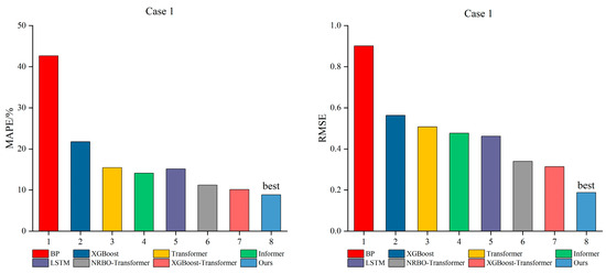
Figure 15. Comprehensive comparison of the prediction performance of all models for Case 1.

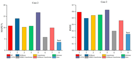
Figure 16. Comprehensive comparison of the prediction performance of all models for Case 2.

Similarly, in Case 2, the differences in errors among the models are relatively reduced. However, the “best” label still firmly belongs to the proposed method in this paper, further demonstrating that the model can maintain good performance across different time scales, data structures, and noise environments.

4.5. Uncertainty Analysis

To further assess the robustness and significance of the proposed NRBO-TXAD model, an uncertainty analysis was conducted on the prediction results of eight models, including the proposed model and seven baseline models, across two case studies. Each model was independently run ten times, and the RMSE and MAPE were calculated for each run. Based on these results, independent-sample t-tests, as defined in Equation (45), were performed to assess the statistical significance of the differences between the proposed model and the others.

$$t={\displaystyle \frac{\overline{x}-\mu }{s/\sqrt{n}}}$$

(45)

where $\overline{x}$, $\mu$, s, and n represent the sample mean, population mean, sample standard deviation, and sample size, respectively. The calculated t-values are presented in Table 12.

Table 12. T-values of statistical significance tests for MAE, RMSE, and MAPE.

Model	Transformer	t Value of Case 1		t Value of Case 2
		MAPE/%	RMSE	MAPE/%	RMSE
BPNN	Single-Step	−21.515	−30.308	−21.145	−18.506
	Two-Step	−29.882	−32.474	−22.82	−23.136
	Three-Step	−29.113	−27.094	−22.105	−22.518
XGBoost	Single-Step	−21.065	−24.782	−33.52	−13.109
	Two-Step	−24.262	−25.211	−29.676	−19.603
	Three-Step	−19.64	−20.571	−22.683	−14.869
Transformer	Single-Step	−10.108	−27.52	−22.212	−18.98
	Two-Step	−13.666	−23.255	−21.922	−23.012
	Three-Step	−21.09	−26.422	−21.991	−17.62
Informer	Single-Step	−2.77	−16.783	−27.757	−17.638
	Two-Step	−6.409	−13.239	−26.843	−18.815
	Three-Step	−7.258	−14.299	−26.921	−22.209
NRBO–Transformer	Single-Step	−9.827	−14.724	−29.412	−11.162
	Two-Step	−15.23	−19.183	−27.564	−20.168
	Three-Step	−13.33	−20.62	−20.724	−19.332
LSTM	Single-Step	−6.827	−23.465	−14.914	−4.69
	Two-Step	−11.793	−18.7	−10.084	−3.979
	Three-Step	−13.61	−18.691	−9.547	−4.068
XGBoost–Transformer	Single-Step	−1.533	−15.683	−32.052	−8.511
	Two-Step	−4.759	−11.455	−20.995	−16.95
	Three-Step	−5.85	−12.849	−20.35	−18.059

Based on the calculated t value, the confidence interval is calculated using Equation (46):

$$IC=\overline{x}\pm t_{\alpha /2,n-1}·s/\sqrt{n}$$

(46)

where $\alpha$ denotes the significance level, which is set to 0.05 for a 95% confidence interval. The 95% confidence intervals for Case 1 and Case 2 are presented in Table 13 and Table 14, respectively.

Table 13. The 95% confidence interval of each model of Case 1.

Model	Single-Step		Two-Step		Three-Step
	MAPE/%	RMSE	MAPE/%	RMSE	MAPE/%	RMSE
BPNN	(−28.605, −23.515)	(−0.455, −0.396)	(−36.497, −31.703)	(−0.818, −0.719)	(−44.259, −38.301)	(−1.018, −0.872)
XGBoost	(−9.799, −8.021)	(−0.226, −0.191)	(−15.962, −13.418)	(−0.487, −0.412)	(−16.737, −13.503)	(−0.515, −0.419)
Transformer	(−4.735, −3.105)	(−0.227, −0.195)	(−7.903, −5.797)	(−0.343, −0.286)	(−9.973, −8.166)	(−0.468, −0.399)
Informer	(−1.477, −0.203)	(−0.131, −0.102)	(−3.492, −1.768)	(−0.165, −0.12)	(−4.707, −2.593)	(−0.226, −0.168)
NRBO–Transformer	(−4.406, −2.854)	(−0.107, −0.08)	(−7.465, −5.655)	(−0.336, −0.269)	(−10.025, −7.295)	(−0.47, −0.383)
LSTM	(−3.008, −1.592)	(−0.268, −0.224)	(−7.057, −4.923)	(−0.285, −0.227)	(−8.692, −6.368)	(−0.406, −0.324)
XGBoost–Transformer	(−1.17, −0.09)	(−0.128, −0.098)	(−2.436, −0.944)	(−0.133, −0.091)	(−3.506, −1.653)	(−0.18, −0.129)

Table 14. The 95% confidence interval of each model of Case 2.

Model	Single-Step		Two-Step		Three-Step
	MAPE/%	RMSE	MAPE/%	RMSE	MAPE/%	RMSE
BPNN	(−6.607, −5.413)	(−0.338, −0.269)	(−8.016, −6.664)	(−0.391, −0.326)	(−9.166, −7.574)	(−0.398, −0.33)
XGBoost	(−9.522, −8.398)	(−0.184, −0.133)	(−11.661, −10.119)	(−0.32, −0.258)	(−12.554, −10.426)	(−0.333, −0.25)
Transformer	(−7.224, −5.976)	(−0.281, −0.225)	(−6.959, −5.741)	(−0.354, −0.294)	(−7.647, −6.313)	(−0.332, −0.261)
LSTM	(−7.81, −6.711)	(−0.374, −0.294)	(−14.815, −12.665)	(−0.432, −0.345)	(−19.825, −16.955)	(−0.442, −0.366)
Informer	(−7.639, −6.621)	(−0.174, −0.119)	(−7.243, −6.217)	(−0.361, −0.293)	(−8.337, −6.803)	(−0.473, −0.38)
NRBO–Transformer	(−3.206, −2.414)	(−0.074, −0.028)	(−2.332, −1.528)	(−0.069, −0.021)	(−2.282, −1.459)	(−0.077, −0.025)
XGBoost–Transformer	(−6.969, −6.111)	(−0.124, −0.075)	(−7.029, −5.751)	(−0.274, −0.213)	(−6.785, −5.515)	(−0.32, −0.254)

According to the statistical analysis results in Table 13 and Table 14, the 95% confidence intervals of all models do not include zero. This indicates that the constructed model has a significant and stable superiority in predictive performance compared with other models.

4.6. Sensitivity Analysis

To comprehensively evaluate the robustness and generalization capability of the NRBO-TXAD model, we performed sensitivity analyses on critical hyperparameters and tested its resilience to input perturbations. The experiments were conducted separately for Case 1 and Case 2.

4.6.1. Hyperparameter Sensitivity

We varied lr, numHeads, and l2 around the optimal point determined by the NRBO for Case 1 and Case 2, and we observed the forecasting performance on the three-step setting. The results in Table 15 and Table 16 show that the performance of NRBO-TXAD deteriorates as hyperparameters deviate from the NRBO-optimized set (Opt-1 and Opt-2).

Table 15. Hyperparameter sensitivity analysis for Case 1.

Case	lr	numHeads	l2	MAPE (%)	RMSE
Opt-1	0.00578	8	0.0001002	11.24	0.2551
Var-1	0.00450	6	0.0010000	13.39	0.3172
Var-2	0.00720	2	0.0000500	15.02	0.3604
Var-3	0.00900	4	0.0005000	14.85	0.3491

Table 16. Hyperparameter sensitivity analysis for Case 2.

Case	lr	numHeads	l2	MAPE (%)	RMSE
Opt-2	0.00629	3	0.0001000	4.90	0.2976
Var-1	0.00500	5	0.0000500	6.67	0.3457
Var-2	0.00750	2	0.0010000	7.89	0.3842
Var-3	0.00820	4	0.0003000	6.21	0.3525

4.6.2. Input Perturbation Sensitivity

To evaluate the robustness of NRBO-TXAD to input uncertainty, we introduced Gaussian noise of varying intensities into the normalized input data, which are low noise (σ = 0.01), moderate noise (σ = 0.05), high noise (σ = 0.10), and severe noise (σ = 0.20), respectively.

As shown in in Table 17, both datasets exhibit a graceful degradation in performance under slight (σ = 0.01) and moderate noise (σ = 0.05), with only minor increases in MAPE and RMSE. This highlights capacity of the model to tolerate real-world measurement inaccuracies. However, under strong (σ = 0.10) and severe noise (σ = 0.20), the prediction error increases significantly, where we reach the limits of noise resilience.

Table 17. Sensitivity to input perturbations with varying Gaussian noise levels.

Dataset	Noise Std (σ)	Description	MAPE (%)	RMSE
Case 1	0	Clean input	11.24	0.2551
	0.01	Slight noise	11.63	0.2640
	0.05	Moderate noise	12.87	0.2873
	0.10	Strong noise	15.42	0.3415
	0.20	Severe noise	22.13	0.4812
Case 2	0	Clean input	4.90	0.2976
	0.01	Slight noise	5.12	0.3028
	0.05	Moderate noise	5.78	0.3260
	0.10	Strong noise	8.94	0.3917
	0.20	Severe noise	14.28	0.5526

4.7. Real-World Applicability and Computational Cost

To assess the real-world deployment potential of the NRBO-TXAD model, we evaluated both its computational efficiency and practical relevance in wind energy systems. We recorded the training time per epoch and average inference time per instance for all models under the same hardware configuration detailed in Section 3.3. Although the NRBO-TXAD model incurs a slightly longer training time due to NRBO-based hyperparameter tuning and dual-module fusion, its inference time remains competitive according to Table 18. Given its accuracy and robustness, it can be integrated into practical deployment although it has one of the longest runtimes. In a typical wind energy SCADA environment, wind speed measurements are received every few minutes. NRBO-TXAD can process the data in real time, predict future wind speeds, and inform turbine yaw control or energy storage dispatch decisions. Moreover, the training can be scheduled offline (e.g., nightly or weekly) to refresh the model parameters with the latest operational data.

Table 18. Comparison of training and inference time.

Model	Case 1		Case 2
	Training Time (s/Epoch)	Inference Time (ms/Instance)	Training Time (s/Epoch)	Inference Time (ms/Instance)
BP Neural Network	0.41	0.32	0.46	0.37
XGBoost	0.58	0.24	0.58	0.28
LSTM	1.25	0.47	1.29	0.48
Transformer	1.38	0.35	1.30	0.31
Informer	1.65	0.42	1.74	0.49
NRBO–Transformer	2.17	0.38	2.13	0.35
XGBoost–Transformer	1.82	0.36	1.66	0.30
Ours	2.35	0.41	2.29	0.38

5. Conclusions

This paper proposes a novel hybrid wind speed forecasting model, NRBO-TXAD, which integrates an NRBO, Transformer network, and XGBoost-based error compensation module. To enhance data quality, IQR-based outlier detection combined with an AMAF was introduced, effectively denoising and smoothing the input series. The NRBO algorithm was used to optimize critical hyperparameters of the Transformer, enabling faster convergence and better generalization. Additionally, XGBoost compensated for nonlinear residual errors, improving the prediction robustness. Extensive experiments on two real-world datasets demonstrated the model’s superior performance over seven baseline methods. The proposed model achieved the lowest prediction errors, with MAPE reduced to 11.24% and RMSE to 0.2551 in Case 1 and with MAPE reduced to 4.90% and RMSE to 0.2976 in Case 2. Moreover, the model exhibited remarkable stability in multi-step forecasting scenarios, exhibiting its robustness and adaptability to different data characteristics and sampling intervals. Specifically, in multi-step forecasting, the model maintained low error rates across different time horizons, with minimal increases in MAPE and RMSE as the prediction steps increased. For example, in Case 2, the single-step prediction MAPE was as low as 2.32%, and even in three-step prediction, it remained at 4.90%. The RMSE only slightly increased from 0.2173 to 0.2976, highlighting its superior generalization ability and anti-degradation capability.

Despite its effectiveness, this study has limitations. The model has only been tested in simulations. Moreover, it does not currently incorporate uncertainty quantification, such as prediction intervals or probabilistic forecasts. Future work will focus on implementing the model in practical wind energy systems and evaluating its performance on embedded platforms. We also plan to extend the framework to spatiotemporal wind field forecasting and to integrate uncertainty quantification. Additionally, combining ensemble learning with uncertainty modeling is expected to improve interpretability and support reliable power system scheduling and grid stability under high wind energy penetration.

References

- Dablander, F.; Hickey, C.; Sandberg, M.; Zell-Ziegler, C.; Grin, J. Embracing Sufficiency to Accelerate the Energy Transition. Energy Res. Social. Sci. 2025, 120, 103907. [Google Scholar] [CrossRef]
- Sun, Y.; Du, R.; Chen, H. Energy Transition and Policy Perception Acuity: An Analysis of 335 High-Energy-Consuming Enterprises in China. Appl. Energy 2025, 377, 124627. [Google Scholar] [CrossRef]
- Liu, H.; Mi, X.; Li, Y. Smart Deep Learning Based Wind Speed Prediction Model Using Wavelet Packet Decomposition, Convolutional Neural Network and Convolutional Long Short Term Memory Network. Energy Convers. Manag. 2018, 166, 120–131. [Google Scholar] [CrossRef]
- Shokri Gazafroudi, A. Assessing the Impact of Load and Renewable Energies’ Uncertainty on a Hybrid System. Int. J. Electr. Power Energy Syst. 2016, 5, 1. [Google Scholar] [CrossRef][Green Version]
- Kim, S.-Y.; Kim, S.-H. Study on the Prediction of Wind Power Generation Based on Artificial Neural Network. J. Inst. Control Robot. Syst. 2011, 17, 1173–1178. [Google Scholar] [CrossRef]
- Qin, X.; Yuan, L.; Dong, X.; Zhang, S.; Shi, H. Short Term Wind Speed Prediction Based on CEESMDAN and Improved Seagull Optimization Kernel Extreme Learning Machine. Earth Sci. Inform. 2025, 18, 141. [Google Scholar] [CrossRef]
- Cai, H.; Wu, Z.; Huang, C.; Huang, D. Wind Power Forecasting Based on Ensemble Empirical Mode Decomposition with Generalized Regression Neural Network Based on Cross-Validated Method. J. Electr. Eng. Technol. 2019, 14, 1823–1829. [Google Scholar] [CrossRef]
- Khan, S.; Muhammad, Y.; Jadoon, I.; Awan, S.E.; Raja, M.A.Z. Leveraging LSTM-SMI and ARIMA Architecture for Robust Wind Power Plant Forecasting. Appl. Soft Comput. 2025, 170, 112765. [Google Scholar] [CrossRef]
- Melalkia, L.; Berrezzek, F.; Khelil, K.; Saim, A.; Nebili, R. A Hybrid Error Correction Method Based on EEMD and ConvLSTM for Offshore Wind Power Forecasting. Ocean. Eng. 2025, 325, 120773. [Google Scholar] [CrossRef]
- Global Wind Energy Council Launched. Refocus 2005, 6, 11. [CrossRef]
- Phan, Q.B.; Nguyen, T.T. Enhancing Wind Speed Forecasting Accuracy Using a GWO-Nested CEEMDAN-CNN-BiLSTM Model. ICT Express 2024, 10, 485–490. [Google Scholar] [CrossRef]
- Countries That Produce the Most Wind Energy. Available online: https://www.evwind.es/2023/01/14/countries-that-produce-the-most-wind-energy/89725 (accessed on 20 April 2025).
- Pinson, P.; Nielsen, H.A.; Madsen, H.; Kariniotakis, G. Skill Forecasting from Ensemble Predictions of Wind Power. Appl. Energy 2009, 86, 1326–1334. [Google Scholar] [CrossRef]
- Barbosa De Alencar, D.; De Mattos Affonso, C.; Limão De Oliveira, R.; Moya Rodríguez, J.; Leite, J.; Reston Filho, J. Different Models for Forecasting Wind Power Generation: Case Study. Energies 2017, 10, 1976. [Google Scholar] [CrossRef]
- Okumus, I.; Dinler, A. Current Status of Wind Energy Forecasting and a Hybrid Method for Hourly Predictions. Energy Convers. Manag. 2016, 123, 362–371. [Google Scholar] [CrossRef]
- Maděra, J.; Kočí, J.; Černý, R. Computational Modeling of the Effect of External Environment on the Degradation of High-Performance Concrete. In AIP Conference Proceedings; American Institute of Physics: Istanbul, Turkey, 2017; Volume 1809, p. 020032. [Google Scholar]
- Georgilakis, P.S. Technical Challenges Associated with the Integration of Wind Power into Power Systems. Renew. Sustain. Energy Rev. 2008, 12, 852–863. [Google Scholar] [CrossRef]
- Pan, J.-S.; Liu, F.-F.; Tian, A.-Q.; Kong, L.; Chu, S.-C. Parameter Extraction Model of Wind Turbine Based on A Novel Pigeon-Inspired Optimization Algorithm. J. Internet Technol. 2024, 25, 561–573. [Google Scholar] [CrossRef]
- Vargas, S.A.; Esteves, G.R.T.; Maçaira, P.M.; Bastos, B.Q.; Cyrino Oliveira, F.L.; Souza, R.C. Wind Power Generation: A Review and a Research Agenda. J. Clean. Prod. 2019, 218, 850–870. [Google Scholar] [CrossRef]
- Shu, Y.; Chen, G.; He, J.; Zhang, F. Building a New Electric Power System Based on New Energy Sources. Chin. J. Eng. Sci. 2021, 23, 61. [Google Scholar] [CrossRef]
- Shahid, F.; Zameer, A.; Muneeb, M. A Novel Genetic LSTM Model for Wind Power Forecast. Energy 2021, 223, 120069. [Google Scholar] [CrossRef]
- Sideratos, G.; Hatziargyriou, N.D. An Advanced Statistical Method for Wind Power Forecasting. IEEE Trans. Power Syst. 2007, 22, 258–265. [Google Scholar] [CrossRef]
- Colak, I.; Sagiroglu, S.; Yesilbudak, M. Data Mining and Wind Power Prediction: A Literature Review. Renew. Energy 2012, 46, 241–247. [Google Scholar] [CrossRef]
- Guo, L.; Xu, C.; Yu, T.; Wumaier, T.; Han, X. Ultra-Short-Term Wind Power Forecasting Based on Long Short-Term Memory Network with Modified Honey Badger Algorithm. Energy Rep. 2024, 12, 3548–3565. [Google Scholar] [CrossRef]
- Bryce, R. Solar PV, Wind Generation, and Load Forecasting Dataset for ERCOT 2018: Performance-Based Energy Resource Feedback, Optimization, and Risk Management (P.E.R.F.O.R.M.); National Renewable Energy Laboratory (NREL): Golden, CO, USA, 2023. [Google Scholar]
- Balkissoon, S.; Fox, N.; Lupo, A.; Haupt, S.E.; Penny, S.G. Classification of Tall Tower Meteorological Variables and Forecasting Wind Speeds in Columbia, Missouri. Renew. Energy 2023, 217, 119123. [Google Scholar] [CrossRef]
- Tian, Z. Modes Decomposition Forecasting Approach for Ultra-Short-Term Wind Speed. Appl. Soft Comput. 2021, 105, 107303. [Google Scholar] [CrossRef]
- Xiong, X.; Zou, R.; Sheng, T.; Zeng, W.; Ye, X. An Ultra-Short-Term Wind Speed Correction Method Based on the Fluctuation Characteristics of Wind Speed. Energy 2023, 283, 129012. [Google Scholar] [CrossRef]
- Saini, V.K.; Kumar, R.; Al-Sumaiti, A.S.; Sujil, A.; Heydarian-Forushani, E. Learning Based Short Term Wind Speed Forecasting Models for Smart Grid Applications: An Extensive Review and Case Study. Electr. Power Syst. Res. 2023, 222, 109502. [Google Scholar] [CrossRef]
- Han, Y.; Mi, L.; Shen, L.; Cai, C.S.; Liu, Y.; Li, K.; Xu, G. A Short-Term Wind Speed Prediction Method Utilizing Novel Hybrid Deep Learning Algorithms to Correct Numerical Weather Forecasting. Appl. Energy 2022, 312, 118777. [Google Scholar] [CrossRef]
- Shirzadi, N.; Nizami, A.; Khazen, M.; Nik-Bakht, M. Medium-Term Regional Electricity Load Forecasting through Machine Learning and Deep Learning. Designs 2021, 5, 27. [Google Scholar] [CrossRef]
- Ávila, L.; Mine, M.R.M.; Kaviski, E.; Detzel, D.H.M. Evaluation of Hydro-Wind Complementarity in the Medium-Term Planning of Electrical Power Systems by Joint Simulation of Periodic Streamflow and Wind Speed Time Series: A Brazilian Case Study. Renew. Energy 2021, 167, 685–699. [Google Scholar] [CrossRef]
- Ban, G.; Chen, Y.; Xiong, Z.; Zhuo, Y.; Huang, K. The Univariate Model for Long-Term Wind Speed Forecasting Based on Wavelet Soft Threshold Denoising and Improved Autoformer. Energy 2024, 290, 130225. [Google Scholar] [CrossRef]
- Hayes, L.; Stocks, M.; Blakers, A. Accurate Long-Term Power Generation Model for Offshore Wind Farms in Europe Using ERA5 Reanalysis. Energy 2021, 229, 120603. [Google Scholar] [CrossRef]
- Omidkar, A.; Es’haghian, R.; Song, H. Using Machine Learning Methods for Long-Term Technical and Economic Evaluation of Wind Power Plants. Green. Energy Resour. 2025, 3, 100115. [Google Scholar] [CrossRef]
- Wang, J.; Che, J.; Li, Z.; Gao, J.; Zhang, L. Hybrid Wind Speed Optimization Forecasting System Based on Linear and Nonlinear Deep Neural Network Structure and Data Preprocessing Fusion. Future Gener. Comput. Syst. 2025, 164, 107565. [Google Scholar] [CrossRef]
- Geng, D.; Zhang, Y.; Zhang, Y.; Qu, X.; Li, L. A Hybrid Model Based on CapSA-VMD-ResNet-GRU-Attention Mechanism for Ultra-Short-Term and Short-Term Wind Speed Prediction. Renew. Energy 2025, 240, 122191. [Google Scholar] [CrossRef]
- Raju, S.K.; Periyasamy, M.; Alhussan, A.A.; Kannan, S.; Raghavendran, S.; El-kenawy, E.-S.M. Machine Learning Boosts Wind Turbine Efficiency with Smart Failure Detection and Strategic Placement. Sci. Rep. 2025, 15, 1485. [Google Scholar] [CrossRef]
- Sanda, M.G.; Emam, M.; Ookawara, S.; Hassan, H. Techno-Enviro-Economic Evaluation of on-Grid and off-Grid Hybrid Photovoltaics and Vertical Axis Wind Turbines System with Battery Storage for Street Lighting Application. J. Clean. Prod. 2025, 491, 144866. [Google Scholar] [CrossRef]
- Xu, H.; Zhao, Y.; Dajun, Z.; Duan, Y.; Xu, X. Exploring the Typhoon Intensity Forecasting through Integrating AI Weather Forecasting with Regional Numerical Weather Model. npj Clim. Atmos. Sci. 2025, 8, 38. [Google Scholar] [CrossRef]
- Han, S.; Song, W.; Yan, J.; Zhang, N.; Wang, H.; Ge, C.; Liu, Y. Integrating Intra-Seasonal Oscillations with Numerical Weather Prediction for 15-Day Wind Power Forecasting. IEEE Trans. Power Syst. 2025, 1–14. [Google Scholar] [CrossRef]
- Duca, V.E.L.A.; Fonseca, T.C.O.; Cyrino Oliveira, F.L. A Generalized Dynamical Model for Wind Speed Forecasting. Renew. Sustain. Energy Rev. 2021, 136, 110421. [Google Scholar] [CrossRef]
- Efthimiou, G.C.; Kumar, P.; Giannissi, S.G.; Feiz, A.A.; Andronopoulos, S. Prediction of the Wind Speed Probabilities in the Atmospheric Surface Layer. Renew. Energy 2019, 132, 921–930. [Google Scholar] [CrossRef]
- Van De Wiel, B.J.H.; Moene, A.F.; Jonker, H.J.J.; Baas, P.; Basu, S.; Donda, J.M.M.; Sun, J.; Holtslag, A.A.M. The Minimum Wind Speed for Sustainable Turbulence in the Nocturnal Boundary Layer. J. Atmos. Sci. 2012, 69, 3116–3127. [Google Scholar] [CrossRef]
- Chenge, Y.; Brutsaert, W. Flux-Profile Relationships for Wind Speed and Temperature in the Stable Atmospheric Boundary Layer. Bound.-Layer. Meteorol. 2005, 114, 519–538. [Google Scholar] [CrossRef]
- Feng, L.; Zhou, Y.; Luo, Q.; Wei, Y. Complex-Valued Artificial Hummingbird Algorithm for Global Optimization and Short-Term Wind Speed Prediction. Expert. Syst. Appl. 2024, 246, 123160. [Google Scholar] [CrossRef]
- Castorrini, A.; Gentile, S.; Geraldi, E.; Bonfiglioli, A. Increasing Spatial Resolution of Wind Resource Prediction Using NWP and RANS Simulation. J. Wind. Eng. Ind. Aerodyn. 2021, 210, 104499. [Google Scholar] [CrossRef]
- Wu, C.; Huang, H.; Zhang, L.; Chen, J.; Tong, Y.; Zhou, M. Towards automated 3D evaluation of water leakage on a tunnel face via improved GAN and self-attention DL model. Tunn. Undergr. Space Technol. 2023, 142, 105432. [Google Scholar] [CrossRef]
- Kavasseri, R.G.; Seetharaman, K. Day-Ahead Wind Speed Forecasting Using f-ARIMA Models. Renew. Energy 2009, 34, 1388–1393. [Google Scholar] [CrossRef]
- Chen, W. A novel Tree-augmented Bayesian network for predicting rock weathering degree using incomplete dataset. Int. J. Rock Mech. Min. Sci. 2024, 183, 105933. [Google Scholar] [CrossRef]
- Torres, J.L.; García, A.; De Blas, M.; De Francisco, A. Forecast of Hourly Average Wind Speed with ARMA Models in Navarre (Spain). Sol. Energy 2005, 79, 65–77. [Google Scholar] [CrossRef]
- Liu, M.-D.; Ding, L.; Bai, Y.-L. Application of Hybrid Model Based on Empirical Mode Decomposition, Novel Recurrent Neural Networks and the ARIMA to Wind Speed Prediction. Energy Convers. Manag. 2021, 233, 113917. [Google Scholar] [CrossRef]
- Jiang, Y.; Huang, G.; Peng, X.; Li, Y.; Yang, Q. A Novel Wind Speed Prediction Method: Hybrid of Correlation-Aided DWT, LSSVM and GARCH. J. Wind. Eng. Ind. Aerodyn. 2018, 174, 28–38. [Google Scholar] [CrossRef]
- García, I.; Huo, S.; Prado, R.; Bravo, L. Dynamic Bayesian Temporal Modeling and Forecasting of Short-Term Wind Measurements. Renew. Energy 2020, 161, 55–64. [Google Scholar] [CrossRef]
- Ak, R.; Fink, O.; Zio, E. Two Machine Learning Approaches for Short-Term Wind Speed Time-Series Prediction. IEEE Trans. Neural Netw. Learning Syst. 2016, 27, 1734–1747. [Google Scholar] [CrossRef] [PubMed]
- Abdelghany, E.S.; Farghaly, M.B.; Almalki, M.M.; Sarhan, H.H.; Essa, M.E.-S.M. Machine Learning and Iot Trends for Intelligent Prediction of Aircraft Wing Anti-Icing System Temperature. Aerospace 2023, 10, 676. [Google Scholar] [CrossRef]
- Wu, C.; Huang, H.; Ni, Y.-Q.; Zhang, L.; Zhang, L. Evaluation of Tunnel Rock Mass Integrity Using Multi-Modal Data and Generative Large Models: Tunnelrip-Gpt. SSRN, 2025; preprint. [Google Scholar] [CrossRef]
- Duan, J.; Chang, M.; Chen, X.; Wang, W.; Zuo, H.; Bai, Y.; Chen, B. A Combined Short-Term Wind Speed Forecasting Model Based on CNN–RNN and Linear Regression Optimization Considering Error. Renew. Energy 2022, 200, 788–808. [Google Scholar] [CrossRef]
- Xu, M. Comparative Analysis of Machine Learning Models for Weather Forecasting: A Heathrow Case Study. TE 2024, 1, 1–12. [Google Scholar] [CrossRef]
- Ren, C.; An, N.; Wang, J.; Li, L.; Hu, B.; Shang, D. Optimal Parameters Selection for BP Neural Network Based on Particle Swarm Optimization: A Case Study of Wind Speed Forecasting. Knowl.-Based Syst. 2014, 56, 226–239. [Google Scholar] [CrossRef]
- Yu, C.; Li, Y.; Zhang, M. Comparative Study on Three New Hybrid Models Using Elman Neural Network and Empirical Mode Decomposition Based Technologies Improved by Singular Spectrum Analysis for Hour-Ahead Wind Speed Forecasting. Energy Convers. Manag. 2017, 147, 75–85. [Google Scholar] [CrossRef]
- Yang, Y.; Solomin, E.V. Wind Direction Prediction Based on Nonlinear Autoregression and Elman Neural Networks for the Wind Turbine Yaw System. Renew. Energy 2025, 241, 122284. [Google Scholar] [CrossRef]
- Santhosh, M.; Venkaiah, C.; Vinod Kumar, D.M. Ensemble Empirical Mode Decomposition Based Adaptive Wavelet Neural Network Method for Wind Speed Prediction. Energy Convers. Manag. 2018, 168, 482–493. [Google Scholar] [CrossRef]
- Banik, A.; Behera, C.; Sarathkumar, T.V.; Goswami, A.K. Uncertain Wind Power Forecasting Using LSTM-based Prediction Interval. IET Renew. Power Gen. 2020, 14, 2657–2667. [Google Scholar] [CrossRef]
- Nair, K.R.; Vanitha, V.; Jisma, M. Forecasting of Wind Speed Using ANN, ARIMA and Hybrid Models. In Proceedings of the 2017 International Conference on Intelligent Computing, Instrumentation and Control Technologies (ICICICT), Kannur, Kerala State, India, 6–7 July 2017; pp. 170–175. [Google Scholar]
- Liu, W.; Bai, Y.; Yue, X.; Wang, R.; Song, Q. A Wind Speed Forcasting Model Based on Rime Optimization Based VMD and Multi-Headed Self-Attention-LSTM. Energy 2024, 294, 130726. [Google Scholar] [CrossRef]
- Qian, Z.; Pei, Y.; Zareipour, H.; Chen, N. A Review and Discussion of Decomposition-Based Hybrid Models for Wind Energy Forecasting Applications. Appl. Energy 2019, 235, 939–953. [Google Scholar] [CrossRef]
- Mi, X.; Zhao, S. Wind Speed Prediction Based on Singular Spectrum Analysis and Neural Network Structural Learning. Energy Convers. Manag. 2020, 216, 112956. [Google Scholar] [CrossRef]
- Liang, T.; Chai, C.; Sun, H.; Tan, J. Wind Speed Prediction Based on Multi-Variable Capsnet-BILSTM-MOHHO for WPCCC. Energy 2022, 250, 123761. [Google Scholar] [CrossRef]
- Vaswani, A.; Shazeer, N.; Parmar, N.; Uszkoreit, J.; Jones, L.; Gomez, A.N.; Kaiser, L.; Polosukhin, I. Attention Is All You Need. arXiv 2017, arXiv:1706.03762. [Google Scholar]
- Wang, C.; Chen, Y.; Zhang, S.; Zhang, Q. Stock Market Index Prediction Using Deep Transformer Model. Expert. Syst. Appl. 2022, 208, 118128. [Google Scholar] [CrossRef]
- Chandra, A.; Tünnermann, L.; Löfstedt, T.; Gratz, R. Transformer-Based Deep Learning for Predicting Protein Properties in the Life Sciences. eLife 2023, 12, e82819. [Google Scholar] [CrossRef] [PubMed]
- Wu, H.; Xu, J.; Wang, J.; Long, M. Autoformer: Decomposition Transformers with Auto-Correlation for Long-Term Series Forecasting. arXiv 2021, arXiv:2106.13008. [Google Scholar]
- Qu, K.; Si, G.; Shan, Z.; Kong, X.; Yang, X. Short-Term Forecasting for Multiple Wind Farms Based on Transformer Model. Energy Rep. 2022, 8, 483–490. [Google Scholar] [CrossRef]
- Yan, D.; Lu, Y. Recent Advances in Particle Swarm Optimization for Large Scale Problems. J. Auton. Intell. 2018, 1, 22. [Google Scholar] [CrossRef][Green Version]
- Kumar, R.; Kumar, A. Application of Differential Evolution for Wind Speed Distribution Parameters Estimation. Wind. Eng. 2021, 45, 1544–1556. [Google Scholar] [CrossRef]
- Sivanandam, S.N.; Deepa, S.N. (Eds.) Introduction to Genetic Algorithms; Springer: Berlin/Heidelberg, Germany, 2008; ISBN 9783540731894. [Google Scholar]
- Dehghani, M.; Hubalovsky, S.; Trojovsky, P. Northern Goshawk Optimization: A New Swarm-Based Algorithm for Solving Optimization Problems. IEEE Access 2021, 9, 162059–162080. [Google Scholar] [CrossRef]
- Mirjalili, S.; Lewis, A. The Whale Optimization Algorithm. Adv. Eng. Softw. 2016, 95, 51–67. [Google Scholar] [CrossRef]
- Fan, X.; Wang, R.; Yang, Y.; Wang, J. Transformer–BiLSTM Fusion Neural Network for Short-Term PV Output Prediction Based on NRBO Algorithm and VMD. Appl. Sci. 2024, 14, 11991. [Google Scholar] [CrossRef]
- Wu, H.; Meng, K.; Fan, D.; Zhang, Z.; Liu, Q. Multistep Short-Term Wind Speed Forecasting Using Transformer. Energy 2022, 261, 125231. [Google Scholar] [CrossRef]
- Novotný, V.; Štefánik, M.; Ayetiran, E.F.; Sojka, P.; Řehůřek, R. When FastText Pays Attention: Efficient Estimation of Word Representations Using Constrained Positional Weighting. J. Univ. Comput. Sci. 2022, 28, 181–201. [Google Scholar] [CrossRef]
- Sowmya, R.; Premkumar, M.; Jangir, P. Newton-Raphson-Based Optimizer: A New Population-Based Metaheuristic Algorithm for Continuous Optimization Problems. Eng. Appl. Artif. Intell. 2024, 128, 107532. [Google Scholar] [CrossRef]
- Magreñán, A.A.; Argyros, I.K. A Contemporary Study of Iterative Methods: Convergence, Dynamics and Applications; Academic Press: London, UK, 2018; ISBN 9780128092149. [Google Scholar]
- Friedman, J.H. Greedy Function Approximation: A Gradient Boosting Machine. Ann. Statist. 2001, 29, 1189–1232. [Google Scholar] [CrossRef]
- Wang, Y.; Guo, Y. Forecasting Method of Stock Market Volatility in Time Series Data Based on Mixed Model of ARIMA and XGBoost. China Commun. 2020, 17, 205–221. [Google Scholar] [CrossRef]
- Gunawan, R.G.; Handika, E.S.; Ismanto, E. Pendekatan Machine Learning Dengan Menggunakan Algoritma Xgboost (Extreme Gradient Boosting) Untuk Peningkatan Kinerja Klasifikasi Serangan Syn. CoSciTech 2022, 3, 453–463. [Google Scholar] [CrossRef]
- Deng, X.; Ye, A.; Zhong, J.; Xu, D.; Yang, W.; Song, Z.; Zhang, Z.; Guo, J.; Wang, T.; Tian, Y.; et al. Bagging—XGBoost Algorithm Based Extreme Weather Identification and Short-Term Load Forecasting Model. Energy Rep. 2022, 8, 8661–8674. [Google Scholar] [CrossRef]
- Semmelmann, L.; Henni, S.; Weinhardt, C. Load Forecasting for Energy Communities: A Novel LSTM-XGBoost Hybrid Model Based on Smart Meter Data. Energy Inform. 2022, 5, 24. [Google Scholar] [CrossRef]
- Leng, Z.; Chen, L.; Yi, B.; Liu, F.; Xie, T.; Mei, Z. Short-Term Wind Speed Forecasting Based on a Novel KANInformer Model and Improved Dual Decomposition. Energy 2025, 322, 135551. [Google Scholar] [CrossRef]
- Hua, Z.; Yang, Q.; Chen, J.; Lan, T.; Zhao, D.; Dou, M.; Liang, B. Degradation Prediction of PEMFC Based on BiTCN-BiGRU-ELM Fusion Prognostic Method. Int. J. Hydrogen Energy 2024, 87, 361–372. [Google Scholar] [CrossRef]
- Chen, G.; Tang, B.; Zeng, X.; Zhou, P.; Kang, P.; Long, H. Short-Term Wind Speed Forecasting Based on Long Short-Term Memory and Improved BP Neural Network. Int. J. Electr. Power Energy Syst. 2022, 134, 107365. [Google Scholar] [CrossRef]
- Fang, Y.; Wu, Y.; Wu, F.; Yan, Y.; Liu, Q.; Liu, N.; Xia, J. Short-Term Wind Speed Forecasting Bias Correction in the Hangzhou Area of China Based on a Machine Learning Model. Atmos. Ocean. Sci. Lett. 2023, 16, 100339. [Google Scholar] [CrossRef]
- He, K.; Zhang, X.; Ren, S.; Sun, J. Deep Residual Learning for Image Recognition. In Proceedings of the 2016 IEEE Conference on Computer Vision and Pattern Recognition (CVPR), Las Vegas, NV, USA, 27–30 June 2016; pp. 770–778. [Google Scholar]
- Zhou, H.; Zhang, S.; Peng, J.; Zhang, S.; Li, J.; Xiong, H.; Zhang, W. Informer: Beyond Efficient Transformer for Long Sequence Time-Series Forecasting. Assoc. Adv. Artif. Intell. 2021, 35, 11106–11115. [Google Scholar] [CrossRef]
- Shao, B.; Song, D.; Bian, G.; Zhao, Y. Wind Speed Forecast Based on the LSTM Neural Network Optimized by the Firework Algorithm. Adv. Mater. Sci. Eng. 2021, 2021, 4874757. [Google Scholar] [CrossRef]
- Shan, S.; Ni, H.; Chen, G.; Lin, X.; Li, J. A Machine Learning Framework for Enhancing Short-Term Water Demand Forecasting Using Attention-BiLSTM Networks Integrated with XGBoost Residual Correction. Water 2023, 15, 3605. [Google Scholar] [CrossRef]
- Shivam, K.; Tzou, J.-C.; Wu, S.-C. Multi-Step Short-Term Wind Speed Prediction Using a Residual Dilated Causal Convolutional Network with Nonlinear Attention. Energies 2020, 13, 1772. [Google Scholar] [CrossRef]
Disclaimer/Publisher’s Note: The statements, opinions and data contained in all publications are solely those of the individual author(s) and contributor(s) and not of MDPI and/or the editor(s). MDPI and/or the editor(s) disclaim responsibility for any injury to people or property resulting from any ideas, methods, instructions or products referred to in the content. |
© 2025 by the authors. Licensee MDPI, Basel, Switzerland. This article is an open access article distributed under the terms and conditions of the Creative Commons Attribution (CC BY) license (https://creativecommons.org/licenses/by/4.0/).