Abstract
This study proposes a deep learning (DL)-based method for identifying the parameters of equivalent circuit models (ECMs) for lithium-ion batteries using time-series voltage response data from current pulse charge–discharge experiments. The application of DL techniques to this task is presented for the first time. The best-performing baseline model among the recurrent neural network, long short-term memory, and gated recurrent unit achieved a mean absolute percentage error (MAPE) of 0.52073 across the five parameters. Furthermore, more advanced models, including a one-dimensional convolutional neural network (1DCNN) and temporal convolutional networks, were developed using full factorial design (FFD), resulting in substantial MAPE improvements of 37.8% and 30.4%, respectively. The effectiveness of Latin hypercube sampling (LHS) for training data generation was also investigated, showing that it achieved comparable or better performance than FFD with only two-thirds of the training samples. Specifically, the 1DCNN model with LHS sampling achieved the best overall performance, with an average MAPE of 0.237409. These results highlight the potential of DL models combined with efficient sampling strategies.
1. Introduction
This study investigates parameter identification (PI) techniques for equivalent circuit models (ECMs) of lithium-ion batteries (LIBs), emphasizing a data-driven approach based on DL. The widely adopted 1RC and 2RC models are selected for their practicality in battery management systems (BMS). By leveraging DL, this study aims to overcome the limitations of traditional PI methods and enhance the accuracy and adaptability of ECM-based modeling. PI in ECM is crucial for accurately modeling lithium-ion battery behavior, especially as battery conditions change over time and usage. Proper identification ensures reliable state estimation, safety, and performance in battery management systems. The importance of this process is highlighted by its impact on model accuracy, computational efficiency, and the ability to adapt to real-world operating conditions [1]. The 2RC ECM is a widely used approach for modeling the electrical behavior of systems such as lithium-ion batteries. This model is particularly valued for its balance between accuracy and computational simplicity, making it suitable for real-time applications [2]. Accurate parameter identification for 1RC and 2RC ECMs of lithium-ion batteries is critical for effective BMS, enabling precise state estimation and optimal performance [3]. These models, characterized by their simplicity and computational efficiency, rely on various techniques to estimate parameters such as resistance and capacitance.
Commonly used PI techniques include analytical methods, Kalman filter-based methods, time-domain meta-heuristic methods, frequency-domain meta-heuristic methods, least squares, recursive least squares, and hybrid methods. Each technique has its own applicability, strengths, and limitations, which are discussed below. Analytical methods leverage mathematical equations to capture battery behavior, often using high-power pulse current tests to fit voltage responses to exponential functions. These methods excel in systems with linear or well-understood dynamics, providing precise parameter estimates through strategic approximations. For instance, Ding et al. (2019) improved the Thevenin model for electric vehicles, achieving high accuracy in parameter estimation [4]. Similarly, Huang et al. (2020) developed fitting strategies for ECMs, enhancing model precision [5]. Solomeh et al. (2016) focused on temperature estimation, integrating analytical techniques for composite lithium-ion cells [6]. However, these methods struggle with highly nonlinear systems and measurement noise, requiring significant expertise to derive governing equations, which limits their applicability in complex scenarios. Kalman filter-based methods are highly adaptable for real-time parameter estimation, effectively handling uncertainties and dynamic battery behavior. These methods, including extended and unscented Kalman filters, track time-varying parameters like state of charge (SoC). Lai et al. (2018) conducted a comparative study of ECMs, demonstrating Kalman filters’ robustness in SoC estimation [7]. Do et al. (2009) used impedance observers with Kalman filters for accurate parameter tracking [8]. Andre et al. (2010) characterized battery aging, integrating Kalman filters for dynamic updates [9]. Kokala et al. (2015) compared ECMs for electric vehicles, highlighting Kalman filters’ real-time capabilities [10]. Hales et al. (2021) applied isothermal control, enhancing parameter accuracy [11]. Despite their strengths, these methods depend on accurate initial models and noise statistics, with computational demands increasing for large-scale systems, potentially limiting real-time feasibility. Time-domain meta-heuristic methods, such as genetic algorithms and harmony search, optimize parameters by minimizing errors between model predictions and experimental data. These methods handle nonlinearities and large parameter spaces effectively. Nenes et al. (2020) identified parameters for lithium-ion batteries using meta-heuristic approaches [12]. Lai et al. (2018) explored ECMs with optimization algorithms, improving accuracy [7]. Huang et al. (2020) applied meta-heuristic fitting strategies, achieving robust results [5]. Solomeh et al. (2016) integrated time-domain optimization for temperature estimation [6]. Ding et al. (2019) enhanced Thevenin models with meta-heuristic methods [4]. However, these methods are computationally expensive and risk converging to local optima, requiring careful tuning of algorithm parameters. Frequency-domain meta-heuristic methods use techniques like impedance spectroscopy to estimate parameters, offering insights into battery dynamics across frequency ranges. These methods are suitable for offline analysis and complex datasets. Nenes et al. (2020) applied frequency-domain techniques for parameter identification [12]. Lai et al. (2018) compared ECMs, incorporating frequency-domain optimization [7]. Huang et al. (2020) developed frequency-based fitting strategies [5]. Solomeh et al. (2016) used frequency-domain methods for temperature estimation [6]. Ding et al. (2019) improved model accuracy with frequency-domain approaches [4]. While effective for detailed analysis, these methods are computationally intensive and less suited for real-time applications due to their complexity. Least squares methods minimize the sum of squared residuals, excelling in offline estimation with large, reliable datasets. Schweighofer et al. (2003) modeled high-power batteries using least squares, achieving computational efficiency [13]. Samirian et al. (2022) developed novel experimental techniques, enhancing parameter accuracy [14]. Knap et al. (2016) compared ECM parameters, demonstrating least squares’ effectiveness [15]. These methods are less effective in noisy environments, as squared residuals amplify large errors, and they require good initial parameter guesses, limiting their use in dynamic applications. Recursive least squares (RLS) methods enable online estimation by continuously updating parameters, adapting to slow changes like temperature or aging. Kokala et al. (2015) applied RLS for SoC estimation in electric vehicles [10]. Lai et al. (2018) integrated RLS with ECMs, improving adaptability [7]. Huang et al. (2020) used RLS for dynamic parameter updates [5]. Pai et al. (2023) employed decoupled RLS for parameter and SOC estimation [16]. Ding et al. (2019) enhanced Thevenin models with RLS [4]. However, RLS is sensitive to noise and abrupt changes, requiring regularization to maintain stability in high-dimensionality systems. Finally, hybrid methods combine multiple techniques, leveraging their strengths to enhance accuracy and robustness. Huang et al. (2020) integrated Kalman filters and optimization algorithms, achieving superior results [5]. Ding et al. (2019) combined analytical and meta-heuristic methods for improved accuracy [4]. Solomeh et al. (2016) used hybrid approaches for temperature estimation, balancing complexity and performance [6]. While promising, hybrid methods are complex to implement and computationally demanding, requiring expert tuning for practical applications. Online methods, such as Kalman filters and RLS, excel in real-time applications, adapting to dynamic changes but requiring significant computational resources. Offline methods, like least squares and meta-heuristics, offer high accuracy but are less suited for dynamic environments. Time-domain methods focus on temporal data, providing simplicity for real-time use, while frequency-domain methods analyze spectral data, offering detailed insights but increasing complexity. Table 1 summarizes the pros and cons of these methods.

Table 1.
Comparison of different PI methods.
On the other hand, machine learning and DL techniques have become increasingly important in estimating the state of health (SOH) and SOC of batteries, particularly lithium-ion batteries used in applications such as electric vehicles and portable electronics. These techniques offer a data-driven approach to understanding battery behavior, which is crucial for ensuring safe and efficient battery operation [17,18,19,20]. However, to the best of our knowledge, no prior studies have proposed the use of DL methods for parameter identification of ECMs in lithium-ion batteries. In this study, a DL-based approach is proposed for ECM parameter identification. The input features to the model consist of time-series voltage response data generated by current pulse charge–discharge experiments, while the outputs are the parameter values of the components in the ECM. The main contributions of this study are listed as follows:
- This study is the first to propose the use of DL methods for estimating ECM parameters from time-series data. The best-performing baseline model achieved an average mean absolute percentage error (MAPE) across the five parameters of 0.52073%.
- Using full factorial design (FFD), advanced models such as one-dimensional convolutional neural networks (1DCNNs) and the temporal convolutional network (TCN) were further proposed. Compared to the best-performing baseline recurrent neural network (RNN) model, the average MAPE across the five parameters was improved by 30.4% and 37.8%, respectively.
- This study also proposed using Latin Hypercube Sampling (LHS) to generate training datasets for DL models. Compared to FFD, the LHS method achieved better estimation performance while requiring only two-thirds of the training samples needed by FFD. The average MAPE across the five parameters was improved by 34.4%.
The remainder of this paper is organized as follows: Section 2 describes the generation of the training dataset, including the use of FFD, LHS, and Monte Carlo (MC) methods. Section 3 introduces the DL models used in this study, including RNN, long short-term memory (LSTM), gated recurrent unit (GRU), TCN, and 1DCNN. Section 4 presents the simulation and experimental results, along with a quantitative performance comparison. Section 5 discusses the observed results, focusing on model accuracy and the influence of different sampling strategies. Finally, Section 6 concludes the study by summarizing key findings and potential future work.
2. Description of the Generation of Training Dataset
As previously mentioned, the input to the DL model in this study is the voltage response, and the output corresponds to the associated ECM parameters. To achieve this, a custom battery parameter simulation platform is developed to generate the necessary training data. The platform simulates the dynamic behavior of the battery by solving state-space equations and employing integer-order calculus. Figure 1 illustrates the second-order RC equivalent circuit model used in this study. In the diagram, and represent the voltages across the two RC parallel branches, denotes the voltage drop across , is the open-circuit voltage, is the terminal voltage of the battery, and I is the input current. The terminal voltage is given by
where , and .
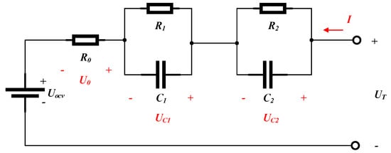
Figure 1.
Second−order RC equivalent circuit model.
The two RC branches in the 2RC model represent distinct electrochemical processes occurring at different time scales within the battery. The first RC branch, characterized by a faster time constant, typically represents the charge transfer resistance and double-layer capacitance at the electrode–electrolyte interface. This branch captures the rapid electrochemical reactions occurring during charge and discharge processes, including activation polarization effects, charge transfer kinetics at the electrode surface, and the formation and dissipation of the electrical double layer. The second RC branch, with a slower time constant, represents diffusion-related processes and other slower electrochemical phenomena. This includes solid-state diffusion of lithium ions within the electrode materials, concentration polarization effects, and mass transport limitations within the porous electrode structure. These processes typically occur over longer time scales compared to the surface reactions. These two branches allow the model to effectively capture the multi-timescale nature of battery dynamics, where fast surface reactions occur simultaneously with slower bulk diffusion processes. This dual-branch approach provides significantly better accuracy in representing the complex impedance characteristics observed in electrochemical impedance spectroscopy measurements across different frequency ranges.
To generate the training data, this study first employed an FFD to generate ECM voltage responses and waveforms. The simulation was performed over a time range from 0 to 660 s with a time step of 0.1 s. To facilitate the simulation of varying input currents, data were recorded every 10 time steps. The input current profile is shown in Figure 2a, where a positive current indicates discharge, and a negative current indicates charge. The factors and their corresponding ranges used in this study are as follows: ranges from 0.020 to 0.050 , from 0.012 to 0.018 , from 0.008 to 0.010 , from 2000 to 3000 F, and from 25000 to 30000 F. The design ranges of these parameters are mainly derived from [21]. Each parameter was discretized into five levels within its specified range, resulting in a total of parameter combinations. The corresponding voltage responses for all parameter sets are shown in Figure 2b.
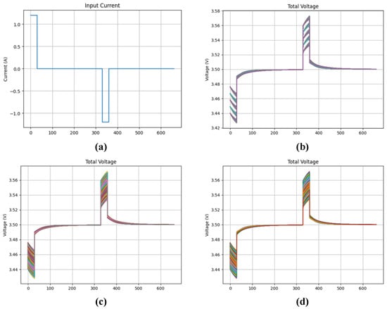
Figure 2.
(a) Input current profile; (b) Simulated voltage responses of FFD; (c) LHS; (d) waveform generated by the MC method.
FFD represents a comprehensive experimental strategy wherein all possible combinations of factor levels are systematically investigated. This methodology is employed to elucidate the main effects of individual factors on a measured response, as well as to quantify the interaction effects between these factors. For a design consisting of k factors, where the j-th factor possesses levels, the total number of unique experimental runs, denoted as N, is determined by the product of the number of levels for each factor:
In the specific instance where all factors exhibit an identical number of levels, L, this equation simplifies to . While FFD ensures a thorough exploration of the experimental space and complete characterization of interactions, its practical implementation can become resource-prohibitive due to the exponential growth in the required number of runs as k or L increases. DL methods require separate training and testing datasets. To evaluate the impact of sampling methods on model accuracy, this study also employs LHS to generate 2048 training data points. LHS is a stratified sampling technique designed to efficiently generate representative samples from a multidimensional parameter space. It offers improved coverage over simple random sampling for a given number of samples. The procedure involves dividing the range of each of the k input variables into N equiprobable, non-overlapping intervals. Subsequently, a single sample value is drawn randomly from each stratum for every variable. These individually sampled values are then combined randomly to form N k-dimensional sample points, with the constraint that, when projected onto any single variable axis, each stratum contains precisely one sample. Although a singular, concise equation does not define LHS in the same manner as FFD, its fundamental principle ensures that each marginal distribution is uniformly sampled. This property makes LHS particularly advantageous for computer experiments and sensitivity analyses where exhaustive exploration is infeasible. Finally, voltage response patterns were generated using the MC method to simulate test data, with parameter ranges identical to those of the original training dataset. MC methods encompass a broad class of computational algorithms that rely on repeated random sampling to obtain numerical solutions. These techniques are particularly powerful for analyzing complex systems characterized by inherent stochasticity or those that are analytically intractable. A primary application of MC sampling is the estimation of the expected value of a random variable or the approximation of an integral. To estimate the expectation E[X] of a random variable X, N independent and identically distributed samples are drawn from the probability distribution of X. The sample mean, , serves as an estimator for :
3. Description of the Deep Learning Models Used in This Study
Since the input data are time-series sequences, this study first employs an RNN as the baseline model. RNNs are DL architectures specifically designed for processing sequential data. They are well-suited for tasks involving temporal dependencies and have been widely applied in various domains, such as natural language processing, speech recognition, and time-series forecasting. Their effectiveness in these tasks is largely due to their inherent “memory” capability, which allows them to retain and utilize information from previous inputs. This memory is enabled by the recurrent structure of the network [22], which allows information to be passed across different time steps.
At its heart, an RNN processes sequential data by maintaining a hidden state that evolves over time. For each input at time step t, the RNN updates its hidden state using the previous hidden state and the current input. This update is typically governed by
where and are weight matrices, is a bias vector, and f is a nonlinear activation function like tanh or ReLU. To produce an output , another linear transformation is often applied:
This simple yet powerful architecture allows the network to learn dependencies across the sequence.
The LSTM network, proposed by Hochreiter and Schmidhuber in 1997, was developed to address the gradient vanishing problem commonly encountered in traditional RNNs. At the core of LSTM is the memory cell, which is regulated by three types of gates:
- Input Gate: Determines how much of the current input should be stored in the memory cell.
- Forget Gate: Decides how much of the information from the previous time step should be retained.
- Output Gate: Controls the output of the memory cell at the current time step.
These gates are all learnable components and dynamically regulate the flow of information based on the content of the input sequence.
The LSTM operates through three primary phases: the forget, input, and output stages. These mechanisms effectively address the vanishing gradient problem and capture long-term dependencies that traditional RNNs struggle with. The forget gate determines how much information from the previous memory state should be discarded. The input gate decides how much of the current input should be retained and used to update the memory cell. Finally, the output gate generates the output at the current time step based on the updated cell state. The equations of the LSTM model are presented in Equations (6) to (11).
The architecture of the GRU and LSTM is shown in Figure 3. The GRU is another type of RNN architecture designed to address the vanishing gradient problem encountered by traditional RNNs when processing long sequences. Like the LSTM network, the GRU is specifically structured to capture long-term dependencies. However, its architecture is more streamlined than that of LSTM, utilizing fewer gates while still achieving comparable performance across many tasks [23]. The equations of the LSTM model are presented in Equations (12) to (15).
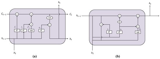
Figure 3.
Structural comparison of LSTM and GRU units. (a) LSTM with input, forget, and output gates. (b) GRU with update and reset gates.
As a simplified variant of the LSTM, the GRU maintains comparable performance while achieving improved computational efficiency through its more streamlined architecture. Both the GRU and LSTM effectively address the vanishing gradient problem inherent in traditional RNNs through their gating mechanisms. This capability gives them a significant advantage in handling long sequence data and capturing long-term dependencies.
In addition to the three RNN-based models, this study also incorporates two novel architectures capable of processing sequential data—the TCN [24] and 1DCNN [25]. TCNs are deep learning architectures designed for sequential data analysis, leveraging 1D convolutional layers to capture temporal patterns efficiently. Unlike RNNs, TCNs process entire sequences in parallel, avoiding sequential computation bottlenecks and enabling faster training. Figure 4 shows the block diagram of a typical TCN, which often includes residual connections to facilitate the flow of information through deep networks and stabilize training. These connections add the input of a block to its output. Additionally, the convolutional layers are usually followed by non-linear activation functions. TCNs have shown promising results in various sequence modeling tasks, sometimes outperforming recurrent networks while offering benefits in terms of parallel computation and gradient stability. They provide a powerful convolutional approach to understanding temporal data.
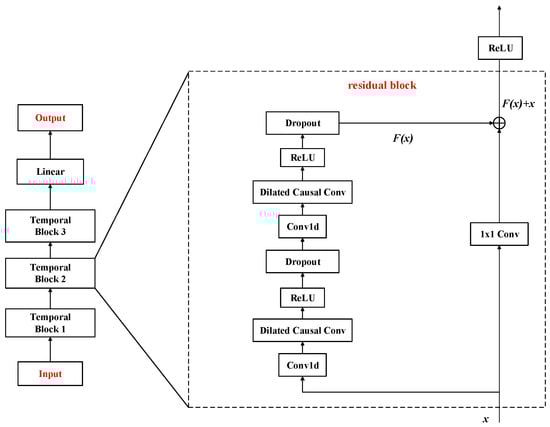
Figure 4.
Block diagram of TCN.
A 1DCNN is a type of neural network primarily designed to process one-dimensional sequential data. Unlike its 2D counterpart that excels in image analysis, a 1DCNN is adept at finding patterns in data that have a temporal or sequential structure, such as time series data and audio signals. It achieves this by employing one-dimensional convolutional layers that slide filters along the data sequence, identifying local patterns. These patterns are then aggregated through subsequent layers to understand the overall structure and make predictions or classifications based on the input sequence.
A typical configuration of a 1DCNN is shown in Figure 5. It starts with an input layer that accepts one-dimensional data. This is followed by one or more convolutional layers, each consisting of a set of learnable filters that convolve across the input sequence. The size of these filters determines the length of the local patterns they can detect. After convolution, a nonlinear activation function, such as ReLU, is applied element-wise to the output. To reduce the dimensionality and provide some translation invariance, pooling layers (like max pooling or average pooling) are often included after the convolutional layers. This process of convolution, activation, and pooling can be repeated multiple times to learn hierarchical features from the data. Finally, the learned features are flattened and passed to one or more fully connected layers, culminating in the final output layer.
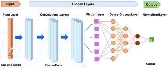
Figure 5.
Block diagram of the 1DCNN.
4. Simulation and Experimental Results
Table 2 lists the hyperparameters of the utilized DL models. As the DL model in this study outputs five circuit parameter values for the ECM, and assuming equal importance for these parameters, the model’s evaluation criterion is the average of their error values. However, given the substantial differences in the scales of these circuit parameters (e.g., resistance on the order of m and capacitance on the order of 1000 F), this study adopts the average MAPE of the five parameters as the performance metric. The definition of MAPE is given in Equation (16).
Table 2.
List of the hyperparameters of the deep learning models utilized.
In Equation (16), is the actual value, is the predicted value, and n is the total number of observations. Figure 6, Figure 7, Figure 8, Figure 9, Figure 10, Figure 11, Figure 12, Figure 13, Figure 14 and Figure 15 present the test set prediction results of the five DL methods under different sampling strategies. In Figure 6, Figure 7, Figure 8, Figure 9 and Figure 10, subfigure (a) shows the box plots of predicted versus actual values for the five parameters when training with FFD sampling, while subfigure (b) shows the corresponding box plots of the prediction errors. Figure 11, Figure 12, Figure 13, Figure 14 and Figure 15 present the results obtained using LHS sampling. Finally, the MAPE results for each method trained with different sampling strategies are summarized in Table 2, Table 3 and Table 4. Figure 16 presents the MAPE sensitivity analysis for all methods.
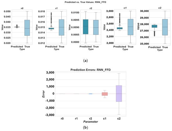
Figure 6.
Prediction results for RNN using FFD sampling: (a) predicted vs. true values, (b) prediction errors.
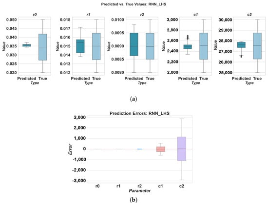
Figure 7.
Prediction results for RNN using LHS sampling: (a) predicted vs. true values, (b) prediction errors.
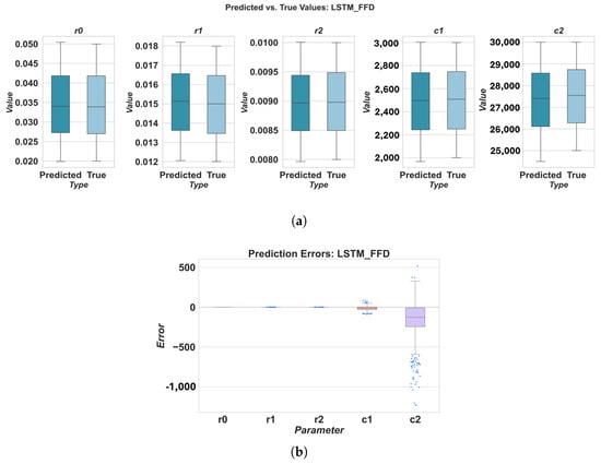
Figure 8.
Prediction results for LSTM using FFD sampling: (a) predicted vs. true values, (b) prediction errors.
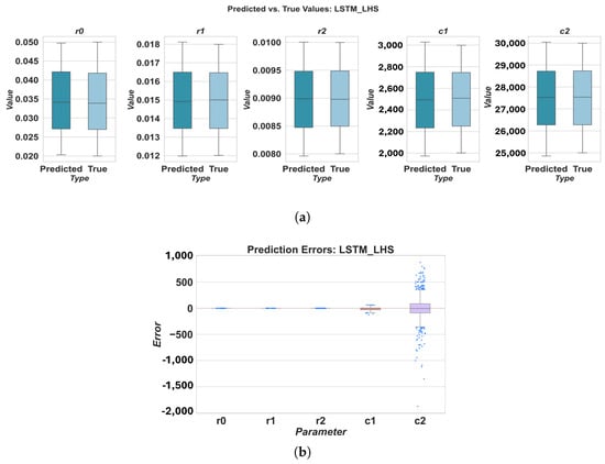
Figure 9.
Prediction results for LSTM using LHS sampling: (a) predicted vs. true values, (b) prediction errors.
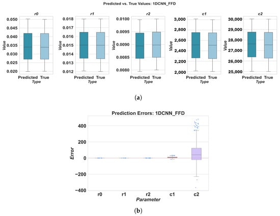
Figure 10.
Prediction results for 1DCNN using FFD sampling: (a) predicted vs. true values, (b) prediction errors.
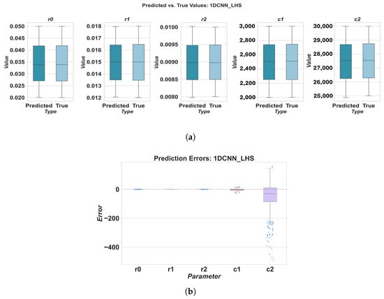
Figure 11.
Prediction results for 1DCNN using LHS sampling: (a) predicted vs. true values, (b) prediction errors.
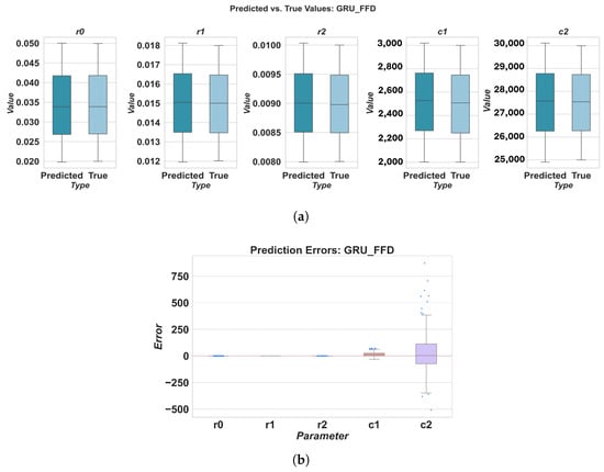
Figure 12.
Prediction results for GRU using FFD sampling: (a) predicted vs. true values, (b) prediction errors.
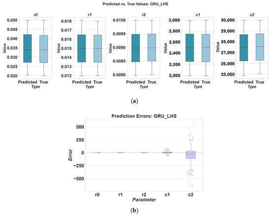
Figure 13.
Prediction results for GRU using LHS sampling: (a) predicted vs. true values, (b) prediction errors.
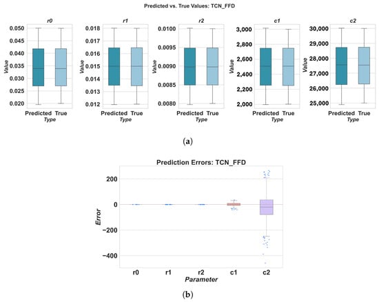
Figure 14.
Prediction results for TCN using FFD sampling: (a) predicted vs. true values, (b) prediction errors.
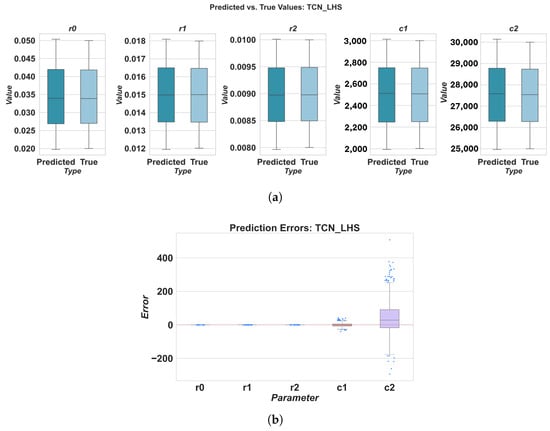
Figure 15.
Prediction results for TCN using LHS sampling: (a) predicted vs. true values, (b) prediction errors.
Table 3.
Comparison of prediction results for the five models using the test set (FFD sampling).
Table 4.
Comparison of prediction results for the four models using the test set (LHS sampling).
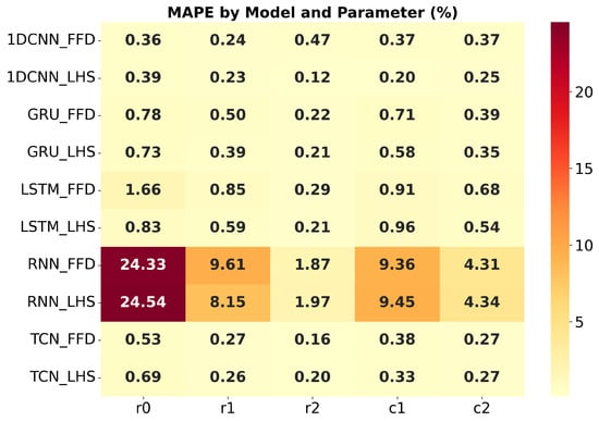
Figure 16.
MAPE sensitivity analysis for all methods.
5. Discussion of the Obtained Results
5.1. Different Model Performance Across Parameters
The results highlight variations in parameter estimation accuracy across different deep learning models and ECM components. For instance, the RNN model generally exhibited the highest MAPE values, particularly for parameters r0, r1, c1, and c2, indicating poorer estimation accuracy compared to other models. Conversely, 1DCNN and TCN consistently demonstrated superior performance across all parameters, with lower MAPE values. This could be attributed to their ability to effectively extract relevant features from the time-series data using convolutional operations. TCN often achieved a low MAPE for parameters like r2. LSTM and GRU showed intermediate performance, with MAPE values generally lower than RNN but higher than 1DCNN and TCN.
5.2. Overall Model Performance
When considering the overall MAPE across all five parameters, 1DCNN and TCN consistently outperformed the other baseline models. With FFD sampling, TCN achieved a good overall MAPE of 0.322106, closely followed by 1DCNN at 0.362589. LHS sampling further improved the performance of 1DCNN, resulting in the lowest overall MAPE of 0.237409 among all models and sampling methods. The RNN model consistently showed the worst overall performance, with MAPE values significantly higher than those of other models, regardless of the sampling method used.
5.3. Impact of Sampling Methods
The choice of sampling method significantly influenced the performance of the deep learning models. LHS generally led to improved or comparable performance compared to FFD. LHS is particularly advantageous as it requires fewer training samples than FFD, making it a more efficient approach for generating training datasets. While FFD provides comprehensive coverage, LHS offers a better balance between coverage and efficiency.
6. Conclusions
This study demonstrates the effectiveness of deep learning techniques for accurate parameter identification of ECMs in lithium-ion batteries. Five deep learning models—RNN, LSTM, GRU, TCN, and 1DCNN—were evaluated under two data sampling strategies: FFD and LHS. The experimental results showed that the RNN model yielded the poorest performance, with average MAPE values exceeding 8 under both sampling methods. In contrast, the proposed 1DCNN and TCN models significantly outperformed the baseline models. The 1DCNN model trained with LHS achieved the best overall performance, with an average MAPE of 0.237409, representing a 54.4% improvement over the best-performing GRU model (MAPE = 0.52073). Moreover, LHS sampling achieved comparable or superior performance to FFD while using only two-thirds of the training data, demonstrating its efficiency. These findings highlight the advantages of combining convolutional deep learning models with efficient sampling strategies for compact, accurate, and data-efficient parameter identification, offering promising potential for integration into real-time battery management systems.
Author Contributions
Conceptualization, Y.-F.H. and K.-C.H.; methodology, Y.-F.H., S.-C.W. and Y.-H.L.; software, D.N.K.; validation, K.-C.H. and D.N.K.; formal analysis, Y.-F.H. and K.-C.H.; writing—original draft, D.N.K. and Y.-F.H.; writing—review & editing, K.-C.H. and S.-C.W.; supervision, K.-C.H. and Y.-H.L. All authors have read and agreed to the published version of the manuscript.
Funding
This research received no external funding.
Data Availability Statement
Data are contained within the article.
Acknowledgments
The authors would like to acknowledge the National Formosa University and the National Taiwan University of Science and Technology for providing the experimental environment and equipment used in this study.
Conflicts of Interest
The authors declare no conflicts of interest.
References
- Lai, X.; Wang, S.; Ma, S.; Xie, J.; Zheng, Y. Parameter sensitivity analysis and simplification of equivalent circuit model for the state of charge of lithium-ion batteries. Electrochim. Acta 2019, 330, 135239. [Google Scholar] [CrossRef]
- Lai, X.; Gao, W.; Zheng, Y.; Ouyang, M.; Li, J.; Han, X.; Zhou, L. A comparative study of global optimization methods for parameter identification of different equivalent circuit models for Li-ion batteries. Electrochim. Acta 2018, 295, 1057–1066. [Google Scholar] [CrossRef]
- Mohamed, M.A.; Yu, T.F.; Ramsden, G.; Marco, J.; Grandjean, T. Advancements in parameter estimation techniques for 1RC and 2RC equivalent circuit models of lithium-ion batteries: A comprehensive review. J. Energy Storage 2025, 113, 115581. [Google Scholar] [CrossRef]
- Ding, X.; Zhang, D.; Cheng, J.; Wang, B.; Luk, P.C.K. An improved Thevenin model of lithium-ion battery with high accuracy for electric vehicles. Appl. Energy 2019, 254, 113615. [Google Scholar] [CrossRef]
- Huang, Y.; Li, Y.; Jiang, L.; Qiao, X.; Cao, Y.; Yu, J. Research on fitting strategy in HPPC test for Li-ion battery. In Proceedings of the 2019 IEEE Sustainable Power and Energy Conference (iSPEC), Chengdu, China, 23–25 November 2019; pp. 1776–1780. [Google Scholar]
- Salameh, M.; Schweitzer, B.; Sveum, P.; Al-Hallaj, S.; Krishnamurthy, M. Online temperature estimation for phase change composite-18650 lithium-ion cells based battery pack. In Proceedings of the 2016 IEEE Applied Power Electronics Conference and Exposition (APEC), Long Beach, CA, USA, 20–24 March 2016; pp. 3128–3133. [Google Scholar]
- Lai, X.; Zheng, Y.; Sun, T. A comparative study of different equivalent circuit models for estimating state-of-charge of lithium-ion batteries. Electrochim. Acta 2018, 259, 566–577. [Google Scholar] [CrossRef]
- Do, D.V.; Forgez, C.; Benkara, K.E.K.; Friedrich, G. Impedance observer for a Li-ion battery using Kalman filter. IEEE Trans. Veh. Technol. 2009, 58, 3930–3937. [Google Scholar]
- Andre, D.; Meiler, M.; Steiner, K.; Walz, H.; Soczka-Guth, T.; Sauer, D.U. Characterization of high-power lithium-ion batteries by electrochemical impedance spectroscopy. II: Modelling. J. Power Sources 2011, 196, 5349–5356. [Google Scholar] [CrossRef]
- Koirala, N.; He, F.; Shen, W. Comparison of two battery equivalent circuit models for state of charge estimation in electric vehicles. In Proceedings of the 2015 IEEE 10th Conference on Industrial Electronics and Applications (ICIEA), Auckland, New Zealand, 15–17 June 2015; pp. 17–22. [Google Scholar]
- Hales, A.; Brouillet, E.; Wang, Z.; Edwards, B.; Samieian, M.A.; Kay, J.; Offer, G. Isothermal temperature control for battery testing and battery model parameterization. SAE Int. J. Electr. Veh. 2021, 10, 105–122. [Google Scholar] [CrossRef]
- Nemes, R.O.; Ciornei, S.M.; Martis, C. Parameters identification using experimental measurements for equivalent circuit Lithium-Ion cell models. In Proceedings of the 2019 11th International Symposium on Advanced Topics in Electrical Engineering (ATEE), Bucharest, Romania, 28–30 March 2019; pp. 1–6. [Google Scholar]
- Schweighofer, B.; Raab, K.M.; Brasseur, G. Modeling of high power automotive batteries by the use of an automated test system. IEEE Trans. Instrum. Meas. 2003, 52, 1087–1091. [Google Scholar] [CrossRef]
- Samieian, M.A.; Hales, A.; Patel, Y. A novel experimental technique for use in fast parameterisation of equivalent circuit models for lithium-ion batteries. Batteries 2022, 8, 125. [Google Scholar] [CrossRef]
- Knap, V.; Stroe, D.I.; Teodorescu, R.; Swierczynski, M.; Stanciu, T. Comparison of parametrization techniques for an electrical circuit model of Lithium-Sulfur batteries. In Proceedings of the 2015 IEEE 13th International Conference on Industrial Informatics (INDIN), Cambridge, UK, 22–24 July 2015; pp. 1278–1283. [Google Scholar]
- Pai, H.Y.; Liu, Y.H.; Ye, S.P. Online estimation of lithium-ion battery equivalent circuit model parameters and state of charge using time-domain assisted decoupled recursive least squares technique. J. Energy Storage 2023, 62, 106901. [Google Scholar] [CrossRef]
- How, D.N.; Hannan, M.A.; Lipu, M.H.; Ker, P.J. State of charge estimation for lithium-ion batteries using model-based and data-driven methods: A review. IEEE Access 2019, 7, 136116–136136. [Google Scholar] [CrossRef]
- Padder, S.G.; Ambulkar, J.; Banotra, A.; Modem, S.; Maheshwari, S.; Jayaramulu, K.; Kundu, C. Data-driven approaches for estimation of EV battery SoC and SoH: A review. IEEE Access 2025, 13, 35048–35067. [Google Scholar] [CrossRef]
- Li, Y.; Liu, K.; Foley, A.M.; Zülke, A.; Berecibar, M.; Nanini-Maury, E.; Hoster, H.E. Data-driven health estimation and lifetime prediction of lithium-ion batteries: A review. Renew. Sustain. Energy Rev. 2019, 113, 109254. [Google Scholar] [CrossRef]
- Gong, J.; Xu, B.; Chen, F.; Zhou, G. Predictive modeling for electric vehicle battery state of health: A comprehensive literature review. Energies 2025, 18, 337. [Google Scholar] [CrossRef]
- Mazumder, M.; Kumar, P.; Ganguly, S. Optimal parameter extraction and performance evaluation of equivalent circuit models for lithium-ion batteries under dynamic conditions. In Proceedings of the 2024 6th International Conference on Energy, Power and Environment (ICEPE), Shillong, India, 20–22 June 2024; pp. 1–6. [Google Scholar]
- Sherstinsky, A. Fundamentals of recurrent neural network (RNN) and long short-term memory (LSTM) network. Phys. D 2020, 404, 132306. [Google Scholar] [CrossRef]
- Mienye, I.D.; Swart, T.G.; Obaido, G. Recurrent neural networks: A comprehensive review of architectures, variants, and applications. Information 2024, 15, 517. [Google Scholar] [CrossRef]
- Lea, C.; Flynn, M.D.; Vidal, R.; Reiter, A.; Hager, G.D. Temporal convolutional networks for action segmentation and detection. In Proceedings of the IEEE Conference on Computer Vision and Pattern Recognition (CVPR), Honolulu, HI, USA, 21–26 July 2017; pp. 156–165. [Google Scholar]
- Sánchez-Reolid, R.; de la Rosa, F.L.; López, M.T.; Fernández-Caballero, A. One-dimensional convolutional neural networks for low/high arousal classification from electrodermal activity. Biomed. Signal Process. Control 2022, 71, 103203. [Google Scholar] [CrossRef]
Disclaimer/Publisher’s Note: The statements, opinions and data contained in all publications are solely those of the individual author(s) and contributor(s) and not of MDPI and/or the editor(s). MDPI and/or the editor(s) disclaim responsibility for any injury to people or property resulting from any ideas, methods, instructions or products referred to in the content. |
© 2025 by the authors. Licensee MDPI, Basel, Switzerland. This article is an open access article distributed under the terms and conditions of the Creative Commons Attribution (CC BY) license (https://creativecommons.org/licenses/by/4.0/).