Abstract
The increasing digitization of educational data poses critical challenges in balancing predictive accuracy with privacy protection for sensitive student information. This study introduces DP-TabNet, a pioneering framework that integrates the interpretable deep learning architecture of TabNet with differential privacy (DP) techniques to enable secure and effective student grade prediction. By incorporating the Laplace Mechanism with a carefully calibrated privacy budget ( = 0.7) and sensitivity ( = 0.1), DP-TabNet ensures robust protection of individual data while maintaining analytical utility. Experimental results on real-world educational datasets demonstrate that DP-TabNet achieves an accuracy of 80%, only 4% lower than the non-private TabNet model (84%), and outperforms privacy-preserving baselines such as DP-Random Forest (78%), DP-XGBoost (78%), DP-MLP (69%), and DP-SGD (69%). Furthermore, its interpretable feature importance analysis highlights key predictors like resource engagement and attendance metrics, offering actionable insights for educators under strict privacy constraints. This work advances privacy-preserving educational technology by demonstrating that high predictive performance and strong privacy guarantees can coexist, providing a practical and responsible framework for educational data analytics.
1. Introduction
The rapid digitization of education has generated unprecedented volumes of student data. This shift is transforming traditional teaching paradigms through predictive analytics. Online learning platforms capture detailed student behaviors, from attendance to interaction frequencies. These data enable advanced models to improve educational outcomes. Convolutional Neural Networks (CNNs) achieve 81–85% accuracy in identifying at-risk students [1]. Integrating Gated Recurrent Units (GRUs) with CNNs further improves temporal and spatial data processing [2]. Text mining methods with semantic analysis further refine grade predictions [3]. Data mining and machine learning methods, such as artificial neural networks, decision trees, and Bayesian learning, are increasingly used to tackle complex academic tasks. These tasks include performance prediction and dropout risk identification [4]. However, handling large amounts of sensitive data requires robust privacy mechanisms. Such mechanisms ensure ethical and responsible use [5,6].
Differential Privacy (DP) adds calibrated noise to datasets or model parameters to protect individual records. This approach provides strong mathematical guarantees [7]. DP has been applied successfully in diverse domains, including federated learning and recommendation systems [8]. It has even been adopted by the U.S. Census Bureau [9]. In educational data mining, DP-based recommendation systems [10] and noise injection in Bayesian networks for grade publication [11] demonstrate practical potential. Recent advancements include differentially private in-context learning for tabular data [12,13]. They also encompass optimized mechanisms for frequency table data release [14]. Comparative studies further demonstrate DP’s superior (, )-bounds over traditional Statistical Disclosure Control (SDC) techniques [15]. Theoretical frameworks also reveal deep connections between DP and computational complexity, cryptography, and learning theory. These frameworks provide a robust foundation for understanding privacy–utility trade-offs [16]. Despite these advances, many methods still struggle to balance privacy and predictive performance. They often sacrifice accuracy or interpretability. For example, DP-TabICL [17] focuses on privacy protection for tabular demonstration data in Large Language Models under the In-Context Learning paradigm. However, this approach differs from integrating DP into specialized tabular learning architectures for predictive modeling.
This study addresses these gaps by introducing DP-TabNet, a novel framework that combines TabNet’s interpretable deep learning architecture with differential privacy techniques. DP-TabNet leverages TabNet’s sequential attention to process high-dimensional tabular data efficiently. It also incorporates the Laplace Mechanism with a calibrated privacy budget ( = 0.7). Together, these features ensure robust data protection and preserve analytical utility. Experimental results on real-world educational datasets show that DP-TabNet achieves 80% accuracy—only 4% lower than the non-private TabNet model (84%). It also outperforms current privacy-preserving baselines.Furthermore, DP-TabNet’s interpretable feature importance analysis provides actionable insights for educators while maintaining strict privacy constraints. This research bridges privacy protection and predictive analytics in educational data mining. It demonstrates the practical integration of DP with deep learning and offers a responsible framework for institutions to leverage data analytics while safeguarding student privacy.
2. Preliminaries
2.1. TabNet Model
TabNet, a deep neural network designed for tabular data, has demonstrated promising results in diverse fields. TabNet outperformed traditional machine learning models in detecting test cheating in education, achieving an AUC of 0.85 [18]. Combined with AdaBoost, the ensemble reached an AUC of 0.92. TabNet accurately predicted the severity of pedestrian crashes in transportation safety by identifying factors such as pedestrian age and lighting conditions [19]. For credit card fraud detection, TabNet surpassed state-of-the-art methods across multiple datasets [20]. Its sequential attention mechanism selects relevant features at each decision step, ensuring interpretability and efficient learning [21].
TabNet effectively handles complex, non-linear relationships in tabular data, making it a valuable tool in education, transportation safety, and finance.
The core architecture of TabNet, shown in Figure 1, includes multiple sequential processing steps, each incorporating feature transformation and selection mechanisms. The feature transformation process is expressed as follows:
where represents the transformed features at step , denotes the feature information from the previous step, is the weight matrix, and is the bias term at step . GLU denotes the Gated Linear Unit activation function.
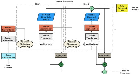
Figure 1.
TabNet architecture.
The architecture includes key components, such as batch normalization for initial feature processing, feature transformers for representation learning, and an attention mechanism for feature selection. The attention mechanism, implemented through a masking layer, determines feature importance scores at each decision step. The feature selection process is governed by:
where denotes the mask at step , is the prior scale from the previous step, and is a sparse alternative to softmax that produces zero probabilities for some inputs. The prior scale is computed as:
where is a relaxation parameter that controls the amount of feature reuse across different decision steps, and denotes the mask values from previous steps.
The attention mechanism transformer, as detailed in Figure 2, plays a crucial role in feature selection and processing.
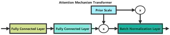
Figure 2.
Attention mechanism transformer.
As shown in Figure 2, the attention mechanism integrates prior scaling and batch normalization, enabling TabNet to dynamically select relevant features, maintain interpretability through explicit feature importance scores, and learn complex patterns while preventing overfitting via controlled feature selection.
The aggregate feature importance for the final prediction is computed as:
where denotes a specific feature, is the number of decision steps, and represents the mask value for feature at step .
This architecture makes TabNet especially well suited for educational data analysis, where prediction accuracy and model interpretability are crucial for practical applications.
2.2. Differential Privacy
Differential Privacy (DP) has emerged as a promising technique for protecting in-dividual privacy in machine learning applications, particularly in education, where sensitive student data must be safeguarded [22,23]. The core principle of DP is to add calibrated noise to data or computations, ensuring that the presence or absence of any individual record cannot be reliably inferred from the analysis results.
Formally, a randomized algorithm satisfies -differential privacy if, for any two adjacent datasets and differing by one record and for any possible output :
where is the privacy budget that governs the privacy-utility trade-off. A smaller provides stronger privacy guarantees but may reduces utility.
In this study, we use the Laplace Mechanism, which adds noise sampled from a Laplace distribution:
where is the sensitivity of the function , defined as:
Sensitivity measures the maximum change in the output when a single record in the input is altered, while represents the desired privacy level. This mechanism provides a mathematical foundation for protecting student data while preserving analytical capabilities, although careful consideration of the privacy-utility trade-off is essential [24].
This brief presentation of DP focuses on the essential concepts and formulas required for the subsequent experimental sections, ensuring logical flow in the paper. The mathematical foundations outlined here will be directly applied to our privacy-preserving TabNet implementation.
3. Experimental Process
Based on the theoretical foundations of TabNet and Differential Privacy outlined previously, we designed and conducted experiments to evaluate the effectiveness of our privacy-preserving student behavior analysis model. This section outlines our experimental methodology, including dataset preparation, model implementation, and the training process.
3.1. Dataset Description and Processing
3.1.1. Dataset Overview
Our study uses a publicly accessible dataset from the Alibaba Cloud Tianchi platform, which contains multi-dimensional data on students’ online learning behaviors and performance records. After carefully selecting features based on their relevance to academic performance, we retained seven key features listed in Table 1:

Table 1.
Feature Descriptions.
These features were selected from an initial set of 17 variables, excluding demo-graphic and administrative data such as gender, nationality, place of birth, and section identifiers, to focus on behavioral indicators directly related to academic performance.
3.1.2. Data Preprocessing
The data preprocessing phase involved three main stages:
First, we performed feature selection by removing non-behavioral attributes (such as gender, nationality, place of birth, state ID, grade ID, topic, semester, relation, and section ID) to focus on learning behavior indicators that directly influence academic performance.
Second, we conducted categorical variable encoding:
- ParentAnsweringSurvey: “Yes” was converted to 1, and “No” was converted to 0;
- ParentschoolSatisfaction: “Good” was converted to 1, and “Bad” was converted to 0;
- StudentAbsenceDays: “Above-7” was converted to 1, and “Under-7” was converted to 0;
- Class: “L” was converted to 0, “M” was converted to 1, and “H” was converted to 2.
Finally, we implemented data standardization and splitting:
- The dataset was divided into training (80%) and testing (20%) sets;
- Feature standardization was applied using StandardScaler to normalize the numerical features;
- Data quality checks were performed to ensure consistency and integrity.
This preprocessing approach ensures that the data is adequately prepared for model training while preserving the essential characteristics of student learning behaviors. Standardization helps optimize the model’s performance by ensuring that all features contribute proportionally to the prediction task.
3.1.3. Ethical Considerations in Data Selection
While the preprocessing steps outlined above ensure data consistency and relevance for predictive modeling, the selection and exclusion of certain features raise important ethical considerations, particularly regarding fairness. In this study, demographic attributes such as gender, nationality, and place of birth were deliberately excluded from the dataset to focus on behavioral indicators of academic performance (e.g., Raisedhands, VisitedResources). However, this exclusion may inadvertently introduce fairness risks by overlooking systemic biases associated with underrepresented groups. For instance, if the data predominantly represent students from specific socioeconomic or cultural backgrounds, the model’s predictions might not generalize equitably across diverse populations, potentially leading to biased outcomes for certain demographics. Such risks could impact the responsible use of predictive models in educational settings, where equitable treatment is paramount. To mitigate these concerns, future iterations of this research will explore the inclusion of fairness-aware techniques, such as reweighting under-represented data or applying fairness constraints during model training, to ensure that the predictive outcomes do not perpetuate existing disparities.
3.2. Implementation of Differential Privacy Preserving Datasets
To protect student privacy, we integrate Differential Privacy (DP) into our data-processing pipeline before model training. We apply the Laplace Mechanism defined in Section 2.2 (Equations (6) and (7)) to perturb the input data. This approach provides (, 0)-DP guarantees. Choosing the privacy budget () and sensitivity () is critical for balancing privacy and data utility. We derive these parameters from rigorous theoretical foundations tailored to sensitive educational data.
We set the privacy budget to 0.7. According to Equation (5) in Section 2.2, this limits an adversary’s ability to distinguish two datasets differing by one record to a factor of . This choice balances strong privacy guarantees with sufficient utility for predictive tasks, safeguarding sensitive educational data.
We analytically determine as the maximum change in the input feature vector caused by altering a single record. This definition is formalized in Equation (7). We standardize features with StandardScaler to achieve zero mean and unit variance. Then, we compute by evaluating the maximum impact of a single data point on the feature distribution. Under a normal distribution, standardized feature values lie within [−3, 3], covering about 99.7% of the data. For the norm, the sensitivity of a single feature equals the maximum change from one record divided by the dataset size. Aggregating across all features, we conservatively set = 0.1 as an upper bound to capture cumulative effects. This choice satisfies DP’s foundational requirement for a theoretically grounded sensitivity measure. We then compute the noise scale for the Laplace mechanism according to Equation (6):
This scale sets the noise magnitude for each feature. Noise is drawn from the Laplace distribution Lap(0, 0.1429) to meet the privacy budget.
We apply the Laplace mechanism to input data before model training. Noise is added independently to each standardized feature in both training and test sets. Noise generation follows the derived scale, strictly enforcing the privacy budget = 0.7 across the entire dataset perturbation. After input perturbation, TabNet’s sequential decision steps incur no additional privacy cost. Applying the privacy budget only at the input level removes the need for composition analysis. This approach ensures a clear, bounded privacy guarantee during data preprocessing. It effectively protects raw data before any model interaction.
Our implementation ensures DP-TabNet adheres to rigorous privacy principles. It also preserves practical utility for educational data analysis. We derive and using formal expressions and precise noise calibration. This process yields a robust privacy-preserving mechanism tailored to sensitive student data. It balances data protection with actionable insights for predictive modeling.
A key design consideration for DP-TabNet is whether TabNet’s sequential decision steps could accumulate privacy budget through iterative processing. In multi-stage architectures, each processing step can be treated as an additional data query. This may require composing privacy budgets under the DP framework. However, DP-TabNet achieves differential privacy by applying the Laplace Mechanism to input data before any model processing. As described earlier, we add noise to standardized features using = 0.7 and = 0.1. This enforces the privacy guarantee at the data level.Subsequent TabNet operations, such as feature selection and transformation, run on perturbed data without accessing the original dataset. As a result, no additional privacy cost occurs during internal processing, and the total budget is bounded by the initial perturbation. This approach ensures TabNet’s multi-step architecture stays within the predefined . It maintains a robust privacy guarantee for the entire framework.
Differential privacy applied via input perturbation with the Laplace Mechanism ( = 0.7, = 0.1) offers strong guarantees against direct exposure of individual data. However, its effectiveness against inference attacks, such as membership inference, where an adversary infers whether a specific record was in the training set, may be a concern during training or deployment. In DP-TabNet, such risks are significantly reduced by input perturbation. We add noise to raw data before any model interaction. This ensures that both the training process and the model parameters derive from perturbed data, inherently obscuring individual contributions. With = 0.7, the privacy guarantee is expressed by the bound . This bound limits an adversary’s ability to distinguish adjacent datasets by about 2.01, providing strong protection against direct re-identification. At this noise level (Lap(0, 0.1429)), inference attacks become less effective. The noise masks identifiable patterns, often reducing adversary confidence to near-random guessing (e.g., 50% for binary membership classification). TabNet’s sequential attention mechanism further mitigates inference risks. By dynamically selecting and processing features, it reduces overfitting to specific data points—a common vulnerability in inference attacks. Although no DP mechanism can eliminate all theoretical risks, DP-TabNet with = 0.7 maintains robust protection during training and deployment. The total privacy budget remains bounded by the initial perturbation, safeguarding sensitive educational data effectively.
3.3. Implementation of TabNet Model
Following the implementation of the differential privacy mechanism, we implemented the TabNet model for both the privacy-preserved and original datasets. The implementation follows the architectural design outlined in Section 2.1, incorporating feature selection and processing mechanisms through sequential attention.
As shown in Figure 3, the TabNet architecture processes student performance features through several sequential steps. The model groups input features into two main categories: Student Classroom Performance (including Raisedhands, VisitedResources, AnnouncementsView, and Discussion) and Student Extracurricular Activities (including ParentAnsweringSurvey, ParentschoolSatisfaction, and StudentAbsenceDays).
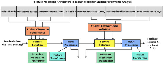
Figure 3.
Feature processing architecture in TabNet model for student performance analysis.
The feature processing flow in Figure 3 illustrates how each feature group undergoes sequential transformations through:
- Feature Selection: using the sparsemax attention mechanism from Equation (2). This selects the most relevant features at each decision step;
- Input Processing: transforming selected features through the Feature Transformer layer as defined in Equation (1);
- Attention Mechanism: the model employs transformers that process features while considering their relationships and importance. The aggregate feature importance is computed using Equation (4);
- Information Aggregation: the processed features from both Student Classroom Performance and Student Extracurricular Activities are aggregated to form comprehensive representations for final prediction.
The feedback loops shown in the diagram implement the feature reuse mechanism controlled by the prior scale as defined in Equation (3).
This implementation allows the model to dynamically select and process features while preserving interpretability through explicit feature importance scores. The architecture’s parameters are carefully tuned, as shown in Table 2, to optimize the model’s performance while preserving computational efficiency.
Table 2.
Parameter descriptions.
The TabNet model architecture is configured with carefully tuned hyperparameters to optimize performance while preserving model efficiency. The key architectural parameters are listed in Table 2:
The key architectural parameters listed in Table 2 are carefully calibrated to optimize the model’s performance:
Learning Rate (lr = 0.001): This value was determined through iterative experimentation within the range [0.0001, 0.01]. The selected learning rate represents an optimal balance between convergence stability and training efficiency. Lower values (≤0.0005) resulted in excessively slow convergence, while higher values (≥0.005) led to oscillation around local minima.
Decision Prediction Layer Width (n_d = 8): This parameter determines the dimensionality of feature transformers in each decision step. We conducted ablation studies with n_d values ranging from 4 to 16 and found that n_d = 8 provides sufficient representational capacity for the educational feature set while preventing overfitting on our dataset size. As formalized in Equation (1), this parameter directly influences the transformation matrix Wi dimensions and consequently affects the model’s capacity to capture complex feature interactions.
Attention Embedding Dimension (n_a = 8): We set n_a equal to n_d to ensure dimensional consistency throughout the network’s attention mechanism. This parameter governs the network’s capacity to focus on relevant features, directly impacting the sparsemax calculations in Equation (2). Our empirical testing showed minimal performance gain with larger values while incurring significant computational overhead.
Number of Decision Steps (n_steps = 3): This value was determined through cross-validation experiments comparing performance with n_steps {2, 3, 4, 5}. With n_steps = 3, the model achieves optimal performance by balancing depth (for capturing complex feature interactions) with parsimony (to prevent overfitting). Adding more steps (n_steps > 3) produced negligible accuracy improvements (<0.7%) while substantially increasing computational complexity. This parameter directly influences the sequential feature selection process described in Equations (2) and (3).
Feature Reuse Coefficient (gamma = 1.2): The γ parameter in Equation (3) governs feature sharing across decision steps. We evaluated performance across the range [1.0, 1.5] at 0.1 increments. The value = 1.2 was selected based on validation performance, as it allows moderate feature reuse while preventing excessive redundancy in feature selection, which is particularly important given the limited dimensionality of our educational dataset.
Number of Independent GLU Layers (n_independent = 2): Three independent Gated Linear Unit layers per step provide sufficient non-linear transformation capacity while preserving model efficiency. This affects the feature transformation process described in Equation (1).
Sparsity Regularization (lambda_sparse = 0.1): This parameter controls the strength of the sparsity constraint on feature selection. The value of 0.1 encourages the model to select relevant features while preventing over-reliance on individual features.
To mitigate overfitting risks from TabNet’s complexity and the small dataset size, we applied 5-fold cross-validation on the training set (80% of the data) prior to final model training. We evaluated using the same hyperparameters as the final model (see Table 2) and applied early stopping based on validation accuracy with a patience of 30 epochs. Cross-validation assesses model generalization and ensures robustness against overfitting—a critical issue when applying deep learning to small datasets.
Figure 3 illustrates the feature processing flow, where each feature group undergoes sequential transformations:
Feature Selection: Applying the Sparsemax attention mechanism (Equation (2)) to select the most relevant features at each decision step.
Input Processing: transforming selected features via the Feature Transformer layer (Equation (1)).
Attention Mechanism: employing transformers to process features based on their relationships and importance, with aggregate importance computed by Equation (4).
Information Aggregation: aggregating processed features from both student classroom performance and extracurricular activities to form comprehensive representations for final prediction.
Feedback loops in the diagram implement the feature reuse mechanism controlled by the prior scale (Equation (3)).
This implementation enables dynamic feature selection and processing, while preserving interpretability via explicit feature importance scores. As shown in Table 2, we carefully tuned the architecture parameters to optimize performance while maintaining computational efficiency.
These hyperparameter values work synergistically to enable effective feature selection and transformation while preserving model interpretability and computational efficiency. The systematic optimization process involved grid search and ablation studies to identify the parameter combination that maximizes predictive performance on educational data while maintaining robust generalization capabilities, as validated through cross-validation.
3.4. Baseline Models
To comprehensively evaluate the performance of our proposed TabNet model, we implemented multiple machine learning algorithms as baseline models, including both traditional tree-based methods and deep learning approaches. These models were chosen for their proven effectiveness in educational data mining and distinct approaches to feature processing and prediction tasks.
Random Forest, an ensemble learning method, constructs multiple decision trees and outputs the class that is the mode of the classes of the individual trees. The model can be represented as:
where is the ensemble predictor, represents individual decision trees, and is the number of trees.
We used RandomizedSearchCV with a predefined parameter space to tune hyperparameters for the Random Forest model and ensure optimal performance. The parameter search space comprised six hyperparameters: number of trees (n_estimators) from 50 to 500; tree depth (max_depth) set to None or 10–90 in steps of 10; minimum samples to split (min_samples_split) from 2 to 20; minimum samples per leaf (min_samples_leaf) from 1 to 20; maximum features for splits (max_features) from 0.1 to 1.0; and bootstrap sampling (bootstrap) either True or False. We performed 100 iterations of randomized search with 5-fold cross-validation, optimizing for accuracy. The optimal hyperparameters were: n_estimators = 393; max_depth = 30; min_samples_split = 3; min_samples_leaf = 3; max_features = 0.23; bootstrap = True. This tuning improved model generalization, as evidenced by cross-validation results.
The Random Forest classifier implementation ensures consistency in predictions through fixed random state initialization while leveraging its advantage in handling both numerical and categorical features present in our educational dataset. The model’s inherent feature importance mechanism provides additional insights into the relative significance of different educational parameters.
XGBoost (eXtreme Gradient Boosting) uses a gradient-boosting decision tree algorithm with additional optimization and regularization techniques. The model follows the principle of additive training:
where is the prediction for the i-th instance, represents the -th tree, and is the space of regression trees.
The objective function being optimized can be expressed as:
where is the loss function and represents the regularization term.
Similarly, we tuned XGBoost hyperparameters with RandomizedSearchCV over 100 iterations and five-fold cross-validation, optimizing for accuracy. The parameter search space included key hyperparameters: number of estimators (n_estimators) from 50 to 600; maximum tree depth (max_depth) from 3 to 10; learning rate (learning_rate) from 0.01 to 1.0; subsample ratio (subsample) from 0.6 to 1.0; column sampling ratio (colsample_bytree) from 0.6 to 1.0; regularization terms (reg_alpha, reg_lambda) from 0 to 1.0; and minimum child weight (min_child_weight) from 1 to 10. The optimal hyperparameters were: n_estimators = 171; max_depth = 7; learning_rate = 0.67; subsample = 0.95; colsample_bytree = 0.75. This selection balances model complexity and performance.
In addition to tree-based models, we implemented a Multilayer Perceptron (MLP) as a representative deep learning baseline. The MLP consists of an input layer, multiple hidden layers with nonlinear activation functions, and an output layer with softmax activation for classification. The forward propagation through the network can be described as:
where is the weighted input to layer , is the weight matrix, is the activation from the previous layer, is the bias vector, and is the activation function.
The MLP model was configured with two hidden layers of 64 and 32 neurons, respectively, using ReLU activation functions and dropout regularization (rate = 0.2) to prevent overfitting. The model was trained using the Adam optimizer with a learning rate of 0.001 and a categorical cross-entropy loss function.
These baseline implementations provide a solid foundation for the comparative analysis presented in Section 4, where we evaluate each approach’s relative strengths and limitations in the context of educational data analysis and privacy preservation. The selection of these diverse baseline models allows for a thorough evaluation of traditional ensemble methods (Random Forest), modern gradient boosting approaches (XGBoost), and neural network architectures (MLP) against the TabNet architecture in both standard and privacy-preserving configurations.
We include Differentially Private Stochastic Gradient Descent (DP-SGD) as an independent privacy-preserving model alongside baseline models evaluated under standard and input-perturbation DP settings. This setup allows us to assess training-time privacy mechanisms. DP-SGD integrates differential privacy into the training process by clipping gradients and adding noise during optimization. This approach provides privacy guarantees at the parameter level instead of the input data level [25]. We implement DP-SGD as a standalone model with a privacy budget of = 0.7 for consistency with the input-perturbation approach used in other models.We tune gradient clipping thresholds and noise scales to balance privacy and utility. However, this method may incur greater computational overhead and degrade performance compared to input perturbation. Including DP-SGD allows comprehensive evaluation of different DP strategies in educational data prediction. It offers insights into their relative impacts on model performance.
4. Results and Analysis
4.1. Performance Evaluation
In this study, we used a comprehensive set of evaluation metrics to assess the performance of the TabNet, Random Forest, and XGBoost models in predicting student grades. The evaluation framework includes primary metrics of accuracy, precision, recall, and F1-score.
The following parameters define these evaluation metrics:
- TP (True Positives): the number of cases where the model correctly predicts the positive class;
- TN (True Negatives): the number of cases where the model correctly predicts the negative class;
- FP (False Positives): the number of cases where the model incorrectly predicts the positive class;
- FN (False Negatives): the number of cases where the model incorrectly predicts the negative class.
Accuracy is a fundamental metric that measures the overall predictive performance of the model. The calculation formula is:
Precision measures the proportion of actual positive samples among the samples predicted as positive, reflecting the model’s ability to avoid false optimistic predictions:
Recall, also known as sensitivity or true positive rate, represents the proportion of actual positive samples that are correctly predicted as positive, indicating the model’s capability to identify all relevant cases:
The F1-score provides a balanced measure of model performance by calculating the harmonic mean of precision and recall. This metric is particularly useful when dealing with imbalanced class distributions, as it considers both false positives and false negatives:
The experimental results demonstrate the comparative performance of each model on the test dataset, as shown in Table 3:
Table 3.
Model comparison.
We obtained an average accuracy of 0.72 (±0.06) across five-fold cross-validation for the non-private TabNet model. This result indicates a potential overfitting risk due to the small dataset size relative to model complexity. The test accuracy of 0.84 indicates that our chosen hyperparameters (Table 2) and regularization techniques partially mitigated this risk. Differences between cross-validation and test performance may stem from data distribution shifts or the limited sample size. This underscores the need for larger datasets in future work to improve model robustness.
The TabNet model achieved superior performance across all evaluation metrics, with an accuracy of 0.84, precision of 0.83, recall of 0.87, and F1-score of 0.85. This performance surpasses the tree-based models (Random Forest and XGBoost) and the deep learning baseline (MLP), with accuracy improvements ranging from 3% to 9%. The high recall value of 0.87 indicates the model’s strong capability to identify students who may require additional academic support or intervention.
Among the baseline models, Random Forest demonstrated the strongest performance with an accuracy of 0.81 and balanced precision and recall scores. XGBoost achieved moderate performance with an accuracy of 0.78, while the MLP model showed the lowest performance with an accuracy of 0.75. The consistent relative performance across different metrics for each model suggests stable and reliable prediction capabilities, although TabNet maintains a clear advantage in overall effectiveness.
The superior performance of TabNet can be attributed to its sophisticated architecture, which incorporates sequential attention mechanisms and dynamic feature selection capabilities, as detailed in Section 2.1. The model’s ability to maintain high performance across all metrics demonstrates its robustness in handling the complexities of educational data.
4.2. Model Interpretability Analysis
Model interpretability is essential for building trustworthy machine-learning systems, especially in sensitive domains such as education. The proposed DP-TabNet model leverages TabNet’s sequential attention mechanism to generate feature importance scores. These scores help educators identify the key predictors of student performance. This subsection evaluates the feature importance scores using a three-step approach. First, we analyze the model’s built-in feature importance derived from its internal mechanism. Second, we validate these scores against ground-truth correlations. Third, we enhance statistical rigor by performing external validation with SHAP values and conducting multicollinearity analysis using the Variance Inflation Factor (VIF). This layered evaluation ensures robust and reliable interpretability.
4.2.1. Built-In Feature Importance via Sparse Attention Mechanism
TabNet computes feature importance using a sparse attention mechanism. At each decision step , a feature mask is generated using Sparsemax, and the aggregate feature importance score for each feature across decision steps is given by:
This formulation enables the model to dynamically select and emphasize relevant features across multiple decision steps while inherently suppressing irrelevant or redundant features through zero-valued masks. The resulting importance scores are directly interpretable and facilitate downstream analysis.
As shown in Figure 4, features such as StudentAbsenceDays, ParentschoolSatisfaction, and VisltedResources are consistently identified as the most influential predictors:
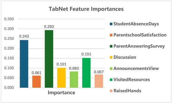
Figure 4.
Feature importance.
Figure 4 shows the relative importance of each feature in DP-TabNet’s predictions. Higher scores correspond to stronger contributions to student grade outcomes. These findings align with pedagogical intuition: attendance (StudentAbsenceDays) and resource engagement (VisitedResources) are critical for academic performance.
4.2.2. Correlation with Ground Truth for Theoretical Grounding
To further validate the model’s interpretability in alignment with established pedagogical literature, we compute the Pearson correlation coefficients between each top-ranked feature and the ground-truth class labels. Given feature and label vector , the Pearson correlation is defined as:
Figure 5 shows that VisitedResources (r = 0.68), Raisedhands (r = 0.65), and AnnouncementsView (r = 0.53) are strongly positively correlated with academic performance. In contrast, Discussion has a lower correlation coefficient (r = 0.31). This suggests that its high importance score in the TabNet model (0.101) may not generalize beyond the training data or may reflect interaction effects with other features (see Section 4.2.3). Additionally, StudentAbsenceDays shows a strong negative correlation (r = −0.67). This aligns with pedagogical expectations that higher absenteeism leads to poorer performance.
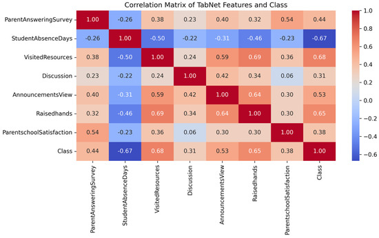
Figure 5.
Correlation matrix and bar plot of top features with “Class”.
These correlation results provide initial theoretical grounding for most of DP-TabNet’s identified key features, reinforcing their relevance in educational contexts. However, correlation alone does not fully capture complex feature interactions or potential model-specific biases in importance rankings, necessitating further validation.
4.2.3. Enhancing Statistical Rigor Through External Validation and Multicollinearity Analysis
First, we use SHAP values to provide a model-agnostic, game-theoretic view of each feature’s contribution to individual predictions. Our 3D SHAP analysis shows that VisitedResources, Raisedhands, and StudentAbsenceDays consistently exert strong influence across performance classes (L, M, H), closely matching DP-TabNet’s internal importance scores (Figure 4). Table 4 and Table 5 summarize SHAP values for the first three samples in each class, illustrating how feature contributions vary. In the low performance class (Class 0 ‘L’), VisitedResources shows strong positive contributions (e.g., SHAP = 0.765 for Sample 1), whereas StudentAbsenceDays shows significant negative contributions (e.g., SHAP = −0.780 for Sample 2). In the high performance class (Class 2 ‘H’), Raisedhands frequently contributes positively (e.g., SHAP = 0.681 for Sample 2). This alignment between built-in and SHAP-derived importance scores reinforces our interpretability analysis, showing that DP-TabNet’s attention mechanism captures meaningful patterns beyond internal biases.
Table 4.
SHAP values summary for across Classes-1.
Table 5.
SHAP values summary for across Classes-2.
We assess multicollinearity using the Variance Inflation Factor (VIF) to prevent artificially inflated importance of correlated predictors. VIF measures how much a regression coefficient’s variance increases due to collinearity with other predictors. Values above 5 indicate potential multicollinearity concerns. Our analysis shows that several engagement-related features exceed this threshold: Raisedhands (VIF = 7.73), VisitedResources (VIF = 7.65), and AnnouncementsView (VIF = 6.33) exhibit the highest collinearity levels. Features with lower VIF values, such as StudentAbsenceDays (VIF = 1.29), demonstrate greater independent predictive power. The complete VIF results are presented in Table 6. Although multicollinearity can affect linear models, DP-TabNet’s non-linear architecture and attention-based feature selection mitigate the impact of correlated features on importance rankings. This analysis confirms that the high importance of key features is not an artifact of collinearity alone. Combining SHAP values with VIF analysis provides a multi-faceted evaluation of feature contributions. This reinforces DP-TabNet’s interpretability reliability for sensitive tasks such as student performance prediction.
Table 6.
Multicollinearity analysis using VIF.
This combined approach of SHAP-based external validation and VIF-based multicollinearity analysis enhances the statistical rigor of our study, ensuring that feature importance rankings are both robust and interpretable. It addresses potential limitations of relying solely on internal mechanisms and provides a multi-faceted understanding of feature contributions in the context of educational data.
4.3. Privacy Protection Effect Analysis
Having established the non-private performance baselines and selected appropriate Differential Privacy parameters ( = 0.7, = 0.1) through empirical evaluation, the impact of applying privacy preservation on model utility is now assessed. The analysis focuses on the performance degradation incurred when models are trained and evaluated on input data perturbed via the Laplace Mechanism using these parameters, alongside an independent training-time privacy mechanism for comparison. Table 7 summarizes the key performance metrics for the Differentially Private (DP) model variants:
Table 7.
Model comparison.
The results presented in Table 7 indicate that the introduction of Differential Privacy through input perturbation affects the candidate models differently. Notably, DP-TabNet maintains the highest predictive performance among the privacy-enhanced models, achieving an accuracy of 0.80 and an F1 score of 0.81. This represents a modest decrease of just 0.04 accuracy compared to its non-private counterpart. TabNet’s relatively high resilience might be attributed to its intrinsic feature selection and sequential attention mechanisms, which could allow it to focus on salient features despite the input noise.
In contrast, the tree-based ensemble models demonstrate varied but generally robust behavior. DP-XGBoost displays remarkable stability, registering no loss in accuracy (0.78) or F1-score (0.78) under these privacy settings, although its overall performance remains below that of DP-TabNet. Similarly, DP-Random Forest shows only a minor accuracy reduction of 0.03, matching DP-XGBoost’s accuracy and F1-score at 0.78. The ensemble nature of these methods likely contributes to their ability to mitigate the effects of the input noise.
The standard Multilayer Perceptron (MLP) architecture appears most vulnerable to privacy-preserving perturbation. DP-MLP experiences the most significant performance decline, with its accuracy dropping by 0.75 to 0.69 and its F1-score falling to 0.68. This suggests that the noise introduced at the input layer may propagate and amplify through the dense network connections, significantly impairing classification accuracy for this standard neural network structure.
DP-SGD, which implements differential privacy by adding noise to gradients during training, shows the lowest performance among the evaluated models. DP-SGD achieves an accuracy of 0.69 and an F1-score of 0.66, representing a 0.15 drop compared with the non-private TabNet baseline. This utility loss likely stems from cumulative noise injection during training, which disrupts optimization and hinders the model’s learning ability.
Overall, our comparative analysis shows that the utility impact of = 0.7 differential privacy depends heavily on the model architecture and the chosen privacy mechanism. While most models maintain reasonable performance under input perturbation, we include DP-SGD as a training-time privacy approach. DP-SGD shows inferior performance, with an accuracy of only 0.69 compared to other models.In contrast, DP-TabNet emerges as the most promising approach. It consistently outperforms all privacy-preserving baselines, including DP-SGD, by delivering superior predictive accuracy while ensuring robust privacy guarantees. These results strongly support using DP-TabNet for sensitive educational data applications, where balancing utility and privacy is crucial.
5. Conclusions
We introduce DP-TabNet, a novel framework integrating TabNet’s interpretable deep learning architecture with differential privacy for student grade prediction. DP-TabNet uses the Laplace Mechanism (ε = 0.7, Δf = 0.1) to provide strong privacy guarantees for sensitive educational data, while preserving analytical utility. On real-world datasets, DP-TabNet achieves 80% accuracy—only 4% lower than the non-private TabNet model (84%). It also outperforms other privacy-preserving baselines: DP-Random Forest and DP-XGBoost (78%), as well as DP-MLP and DP-SGD (69%). DP-TabNet’s interpretability, powered by TabNet’s sequential attention, highlights key predictors: resource engagement (VisitedResources), class participation (Raisedhands), and attendance (StudentAbsenceDays). This provides educators with actionable insights under strict privacy constraints. These results demonstrate that privacy preservation and predictive performance can coexist in educational data mining, offering institutions a practical, ethical analytics solution. Future work will explore adaptive privacy mechanisms to optimize the privacy–utility trade-off and investigate fairness-aware techniques to reduce biases in data selection. We will also extend DP-TabNet to diverse educational applications, including personalized learning and at-risk student identification.
Author Contributions
Conceptualization, Y.Z.; data curation, Q.G.; formal analysis, Y.Z. and Q.G.; funding acquisition, J.W.; methodology, Y.Z.; project administration, J.W.; resources, W.W.; software, Y.Z. and L.W.; supervision, J.W.; validation, Y.Z.; visualization, L.W.; writing—review and editing, Y.Z., J.W., and X.T. All authors have read and agreed to the published version of the manuscript.
Funding
This research was Partly funded by Guangdong Basic and Applied Basic Research Foundation grant number 2024A1515013066, and the Construction Project of Teaching Quality and Teaching Reform in Guangdong Undergraduate Colleges grant number 2022SJZ002, and the Guangdong Province Key Construction Discipline Scientific Research Ability Promotion Project grant number 2022ZDJS133, and the Undergraduate Innovation and Entrepreneurship Training Program Project grant number S202412668030.
Data Availability Statement
The original contributions presented in this study are included in the article. Further inquiries can be directed to the corresponding author.
Conflicts of Interest
The authors declare no conflict of interest.
References
- Zhang, Y.; An, R.; Cui, J.; Shang, X. Undergraduate Grade Prediction in Chinese Higher Education Using Convolutional Neural Networks. In Proceedings of the LAK21: 11th International Learning Analytics and Knowledge Conference, Irvine, CA, USA, 12–16 April 2021. [Google Scholar]
- Zeng, D.; Wu, G.; Pang, S.; Zeng, D.; Chen, X.; Shao, S. A Hybrid Neural Network-based Approach for Predicting Course Grades. In Proceedings of the 2022 3rd International Conference on Information Science and Education (ICISE-IE), Guangzhou, China, 18–20 November 2022. [Google Scholar]
- Li, J.; Supraja, S.; Qiu, W.; Khong, A.W. Grade Prediction via Prior Grades and Text Mining on Course Descriptions: Course Outlines and Intended Learning Outcomes. In Proceedings of the Educational Data Mining, Durham, UK, 24–27 July 2022. [Google Scholar]
- Nájera, A.B.; Mora, J.D. Breve revisión de aplicaciones educativas utilizando Minería de Datos y Aprendizaje Automático. Rev. Electrónica Investig. Educ. 2017, 19, 84–96. [Google Scholar]
- Gursoy, M.E.; Inan, A.; Nergiz, M.E.; Saygin, Y. Privacy-Preserving Learning Analytics: Challenges and Techniques. IEEE Trans. Learn. Technol. 2017, 10, 68–81. [Google Scholar] [CrossRef]
- Ouadrhiri, A.E.; Abdelhadi, A.M. Differential Privacy for Deep and Federated Learning: A Survey. IEEE Access 2022, 10, 22359–22380. [Google Scholar] [CrossRef]
- Zhao, J.; Chen, Y.; Zhang, W. Differential Privacy Preservation in Deep Learning: Challenges, Opportunities and Solutions. IEEE Access 2019, 7, 48901–48911. [Google Scholar] [CrossRef]
- Zhao, J. Distributed Deep Learning under Differential Privacy with the Teacher-Student Paradigm. In Proceedings of the AAAI Workshops, New Orleans, LA, USA, 2–7 February 2018. [Google Scholar]
- Abowd, J.M. The U.S. Census Bureau Adopts Differential Privacy. In Proceedings of the 24th ACM SIGKDD International Conference on Knowledge Discovery & Data Mining, New York, NY, USA, 23 August 2018. [Google Scholar]
- Xu, S.; Yin, X. Recommendation System for Privacy-Preserving Education Technologies. Comput. Intell. Neurosci. 2022, 2022, 3502992. [Google Scholar] [CrossRef] [PubMed]
- Raigoza, J.; Wankhede, D. Publishing Student Grades while Preserving Individual Information Using Bayesian Networks. In Proceedings of the 2016 International Conference on Computational Science and Computational Intelligence (CSCI), Las Vegas, NV, USA, 15–17 December 2016; pp. 1399–1400. [Google Scholar]
- Lee, J.; Kim, M.; Jeong, Y.; Ro, Y. Differentially Private Normalizing Flows for Synthetic Tabular Data Generation. In Proceedings of the AAAI Conference on Artificial Intelligence, Vitural, 22 February–1 March 2022. [Google Scholar]
- Wang, X.; Yu, C.; Chen, P. Exploring the Benefits of Differentially Private Pre-training and Parameter-Efficient Fine-tuning for Table Transformers. arXiv 2023, arXiv:2309.06526. [Google Scholar]
- Li, C.; Wang, N.; Xu, G. Inference for Optimal Differential Privacy Procedures for Frequency Tables. J. Data Sci. 2022, 20, 253–276. [Google Scholar] [CrossRef]
- Das, S.; Zhu, K.; Task, C.; Hentenryck, P.V.; Fioretto, F. Finding ϵ and δ of Statistical Disclosure Control Systems. In Proceedings of the 38th AAAI Conference on Artificial Intelligence, Vancouver, BC, Canada, 20–27 February 2024. [Google Scholar]
- Vadhan, S.P. The Complexity of Differential Privacy. In Tutorials on the Foundations of Cryptography; Springer: Berlin/Heidelberg, Germany, 2017; pp. 347–450. [Google Scholar]
- Carey, A.N.; Bhaila, K.; Edemacu, K.; Wu, X. DP-TabICL: In-Context Learning with Differentially Private Tabular Data. In Proceedings of the 2024 IEEE International Conference on Big Data (BigData), Washington, DC, USA, 15–18 December 2024; pp. 1552–1557. [Google Scholar]
- Zhen, Y.; Zhu, X. An Ensemble Learning Approach Based on TabNet and Machine Learning Models for Cheating Detection in Educational Tests. Educ. Psychol. Meas. 2023, 84, 780–809. [Google Scholar] [CrossRef] [PubMed]
- Rafe, A.; Singleton, P.A. A Comparative Study Using Generalized Ordered Probit, Stacking Ensemble, and TabNet: Application to Determinants of Pedestrian Crash Severity. Data Sci. Transp. 2023, 6, 1–26. [Google Scholar] [CrossRef]
- Meng, C.C.; Lim, K.M.; Lee, C.P.; Lim, J.Y. Credit Card Fraud Detection using TabNet. In Proceedings of the 2023 11th International Conference on Information and Communication Technology (ICoICT), Melaka, Malaysia, 23–24 August 2023; pp. 394–399. [Google Scholar]
- Arik, S.Ö.; Pfister, T. TabNet: Attentive interpretable tabular learning. In Proceedings of the AAAI Conference on Artificial Intelligence, Vitural, 2–9 February 2021; Volume 35, pp. 6679–6687. [Google Scholar]
- Gong, M.; Xie, Y.; Pan, K.; Feng, K.; Qin, A. A Survey on Differentially Private Machine Learning [Review Article]. IEEE Comput. Intell. Mag. 2020, 15, 49–64. [Google Scholar] [CrossRef]
- O’Hara, A.; Straus, S. Privacy Preserving Technologies in US Education. Int. J. Popul. Data Sci. 2022, 7, 2084. [Google Scholar] [CrossRef]
- Blanco-Justicia, A.; Sánchez, D.; Domingo-Ferrer, J.; Muralidhar, K. A Critical Review on the Use (and Misuse) of Differential Privacy in Machine Learning. ACM Comput. Surv. 2022, 55, 1–16. [Google Scholar] [CrossRef]
- Abadi, M.; Chu, A.; Goodfellow, I.J.; McMahan, H.B.; Mironov, I.; Talwar, K.; Zhang, L. Deep Learning with Differential Privacy. In Proceedings of the 2016 ACM SIGSAC Conference on Computer and Communications Security (CCS’16), Vienna, Austria, 24–28 October 2016; pp. 308–318. [Google Scholar]
Disclaimer/Publisher’s Note: The statements, opinions and data contained in all publications are solely those of the individual author(s) and contributor(s) and not of MDPI and/or the editor(s). MDPI and/or the editor(s) disclaim responsibility for any injury to people or property resulting from any ideas, methods, instructions or products referred to in the content. |
© 2025 by the authors. Licensee MDPI, Basel, Switzerland. This article is an open access article distributed under the terms and conditions of the Creative Commons Attribution (CC BY) license (https://creativecommons.org/licenses/by/4.0/).