Stability Analysis and Virtual Inductance Control for Static Synchronous Compensators with Voltage-Droop Support in Weak Grid

Abstract

Static synchronous compensators (STATCOMs) are widely applied in modern power networks for reactive power compensation and grid voltage regulation. Compared to the conventional compensation devices, the STATCOMs deliver superior performance through the voltage-droop control loop. However, the interaction between the STATCOMs and grid impedance, especially in weak grids, can lead to stability issues. To investigate this instability mechanism, the STATCOMs and grid impedance are modeled as a multi-input–multi-output system in this paper. Thus, the coupling effects between the control loop and the grid impedance are clearly highlighted, making the stability assessment feasible. The proposed method avoids the cost and volume issues associated with adding physical inductance in traditional approaches to mitigate these coupling effects. It not only improves the operational stability of the STATCOM but also enhances its voltage support capability, thereby supplementing the stability research for weak grids with STATCOMs under this specific condition. The effectiveness of the presented analysis and proposed control scheme are validated through both simulation and experimental results.

1. Introduction

With the continuous development of renewable energy generation technologies, modern power grids are incorporating increasing numbers of power electronic devices [1,2]. The growing proportion of nonlinear loads has led to power quality degradation in power systems. The excessive penetration of power electronic equipment may cause operational issues, including impaired equipment performance, additional energy losses, and electromagnetic interference [3]. To address power quality challenges, researchers have proposed various compensation devices such as unified power quality conditioners (UPQCs) [4,5], static VAR compensators (SVCs) [6,7], static synchronous compensators (STATCOMs), and dynamic voltage restorers (DVRs) [8,9]. As a power electronics-based flexible AC transmission system (FACTS) device [10,11], STATCOMs operate at both transmission [12] and distribution levels [13], providing voltage stabilization and power quality compensation through reactive power control. In public grid applications, STATCOMs deliver leading or lagging reactive power to maintain transient stability [14,15]. Recent research advancements aiming to enhance STATCOM practicality have been systematically reviewed [16].

Although STATCOM has numerous advantages, it still has the potential to trigger various stability issues. Research has revealed that inter-STATCOM interactions exhibit distinct characteristics compared to conventional converters, primarily mediated through AC voltage control loops instead of phase-locked loops (PLLs) [17]. Recent advancements focus on enhancing STATCOM operational effectiveness through innovative control architectures. A notable development involves a decoupling algorithm that embeds primary control loops within the output feedback path, effectively separating active and reactive current control modes [18]. The PV-STATCOM synthetic topology synergizes the photovoltaic inverter control with reactive power compensation capabilities, effectively suppressing both steady-state voltage rise and transient overvoltage phenomena in high-penetration photovoltaic systems, while exhibiting superior cost–benefit metrics compared to conventional SVC topologies [19].

In addition to the coupling issues caused by multiple power electronic devices, grid impedance can also adversely affect system stability [20,21]. Modern renewable energy power generation systems are typically connected to the power grid at the PCC via the main feeder, thereby synchronizing with the grid’s frequency and voltage [22]. However, during actual implementation, renewable energy power plants are often located far from the main power grid [23,24]. Under such conditions, the grid information measured by the grid-connected equipment of these renewable energy systems can significantly deviate from the characteristics of an ideal power grid [25,26,27]. Consequently, control strategies that are effective under ideal grid conditions may no longer be applicable [28]. This type of power grid is commonly referred to as a “weak grid,” which denotes a sub-grid with weak interconnection to the main power grid.

There is no universally accepted definition of a weak grid [29,30,31]. From a qualitative perspective, such grids are principally characterized by distinct electrical properties, including low short-circuit capacity, elevated grid impedance, reduced mechanical inertia, and inadequate rotational reserves. Quantitatively, the short-circuit ratio (SCR) serves as a prevalent metric for evaluating grid strength, though the critical SCR thresholds proposed in different scholarly works demarcate weak grids may exhibit discrepancies. As per the IEEE Standard 1204-1997 [31], the SCR is mathematically defined as the ratio between the grid’s short-circuit capacity and its rated power capacity. Grid interconnection systems demonstrating an SCR below 3 are conventionally classified as weak grids.

The interaction between a weak grid and power electronic devices can induce multiple stability challenges. Recent studies have developed diverse solutions to address these issues. For instance, a grid voltage feed-forward scheme applicable to grid-connected inverters has been proposed to eliminate background voltage harmonics in microgrids [32]. Furthermore, the impedance analysis method has been employed to systematically investigate the weak grid-modular multilevel converter interaction, quantitatively revealing how grid weakness affects the system stability margin [33]. To address the challenge of high sensitivity in PCC voltage amplitude and phase to large time-varying cyclic load variations in weak grids, a STATCOM control strategy integrated with capacitive energy storage has been designed, demonstrating enhanced adaptability to dynamic load conditions [34]. The high grid impedance in weak grids directly interacts with STATCOM’s voltage droop control dynamics, creating a critical coupling mechanism that this study aims to address.

STATCOMs in power systems inherently modulate the voltage amplitude at the PCC through their reactive power compensation dynamics. While this effect remains negligible in ideal grid conditions with low impedance, it becomes significantly pronounced in weak grid scenarios characterized by high network impedance. To address this operational challenge, voltage droop control is conventionally implemented to regulate PCC voltage within permissible limits and enhance the grid power quality [35]. However, the implementation of droop control introduces an additional feedback control loop into the system architecture. This supplementary loop exhibits frequency-dependent coupling characteristics with grid impedance parameters, potentially inducing oscillatory instabilities or resonance phenomena that may compromise overall grid stability.

Currently, there is a lack of research on the stability of STATCOMs under weak grid conditions. Studies on power oscillations in transmission systems have identified that these oscillations are caused by the coupling effects between STATCOMs and the grid [36]. Time-domain analysis demonstrates that factors such as the number of STATCOMs and the system’s effective short-circuit ratio contribute to instability. However, this work does not provide a detailed modeling of STATCOMs. While some researchers have developed precise STATCOM models to analyze the relationship between STATCOM quantities and system instability, their approach is limited to port impedance models, which fail to reveal the underlying instability mechanisms [35].

To address this research gap, this paper analyzes the transfer function to clarify the coupling mechanism between STATCOMs and the grid, and proposes a virtual inductance control method to mitigate this coupling. Simulations and experiments confirm that the proposed method effectively enhances system stability.

The remainder of this paper is organized as follows. Section 2 describes the system under study. Section 3 analyzes the stability of STATCOMs in weak grids. Section 4 elaborates on the proposed virtual inductance control method. Section 5 presents simulation and experimental results. Section 6 concludes the paper.

2. Introduction of STATCOMs in Weak Grid

This section is an introduction to the circuit topology and basic control methods we have studied. The first section introduces the overall topology and control methods, and the second section provides a fundamental explanation of the drooping control method.

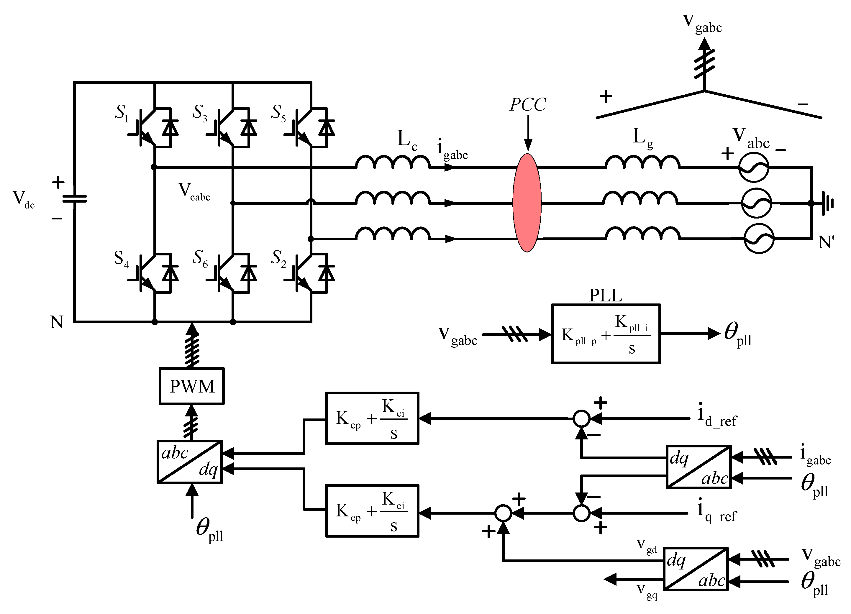
2.1. Basic Operational Principle of STATCOM

As demonstrated in Figure 1, the primary system schematic and control scheme of STATCOM comprises a DC-link voltage $v_{dc}$, a three-phase grid-connected inverter, and three filter inductances $L_c$. It is noteworthy that the subscripts a, b, and c denote three-phase quantities. In the context of this study, the weak grids are modeled as a connection series of an ideal grid voltage $v_{abc}$ and a grid inductance L_g. It is imperative to emphasize that, in scenarios characterized by weak grids (large L_g), as indicated by substantial values of L_g, the voltage drop across L_g becomes pronounced and cannot be disregarded. This results in a substantial discrepancy between the measured PCC voltage $v_{gabc}$ and the ideal grid voltages $v_{abc}$. As illustrated in Figure 1, the system’s control scheme is implemented in the synchronous $dq0$-frame.

As illustrated in Figure 1, the system’s control scheme is implemented in the synchronous $dq0$-frame. It is important to note that d axis or $q$ axis quantities are denoted by the subscripts $d$ or $q$, respectively. Furthermore, the subscript “$ref$” signifies reference notation. The system’s control scheme functions as follows: the initial step involves the measurement of the PCC voltage phase $v_{gabc}$ using a PLL for the transformation between the $abc/dq$ and $dq/abc$ frames. Consequently, the control requirements for voltage and current are transformed into the $dq0$-frame. The droop controller then generates the PCC reference current $i_{cq\_ref}$ through the interaction of $v_{cd}$ and $v_{gd}$. Ultimately, the current controller and PWM ensure that the DC-link voltage $v_{cd}$ tracks the voltage reference adjusted by the droop controller.

2.2. Droop Control

Since this paper modifies the conventional droop control method, this section will introduce the principle of droop control and the implementation approach adopted in this study.

The output impedance of the STATCOM is highly inductive, and the reactive power absorbed by the grid bus can be expressed as [37]

$$Q={\displaystyle \frac{EVcos\phi -V^2}{X}}$$

(1)

Here, E denotes the output voltage of the STATCOM, V represents the voltage at the PCC point, X corresponds to the output reactance of the STATCOM, and $\phi$ indicates the phase angle between E and V.

From this equation, it can be observed that the output voltage E of the STATCOM is directly proportional to its reactive power output Q.

Furthermore, the reactive power in the $dq$-frame can also be expressed as [38]

$$Q=v_q{i}_d-v_d{i}_q$$

(2)

Since the primary function of the STATCOM is to transmit reactive power, the d axis current $i_d$ is set to zero. Consequently, the q axis current $i_q$ is inversely proportional to the reactive power Q, and further inversely proportional to the output voltage E.

Due to the high impedance inherent in weak grids, a certain degree of voltage drop occurs on the transmission lines, causing V to fall below the rated grid voltage. The introduction of droop control aims to elevate E by reducing $i_q$, thereby increasing V, which enhances the support capability for weak grids. The droop control coefficient $K_{vq}$ governs the STATCOM’s support capability, while the specific system impacts of its parameter selection will be analyzed in subsequent sections.

However, providing this support capability comes at a cost—the inability to achieve error-free regulation of reactive power output. Without droop control, the q axis current is controlled to match the reference q axis current $i_{q\_ref}$. However, after introducing droop control, the droop path affects the q axis control loop, preventing the precise tracking of $i_{q\_ref}$ and consequently eliminating the possibility of error-free reactive power output regulation.

3. Stability Analysis of STATCOMs in Weak Grid

This section is the stability analysis of STATCOM under the weak current network. The first section deduces the system control block diagram. The second section, based on this, deduces the expression of the transfer function matrix as the basis for stability analysis. The third section analyzes the system stability from multiple perspectives.

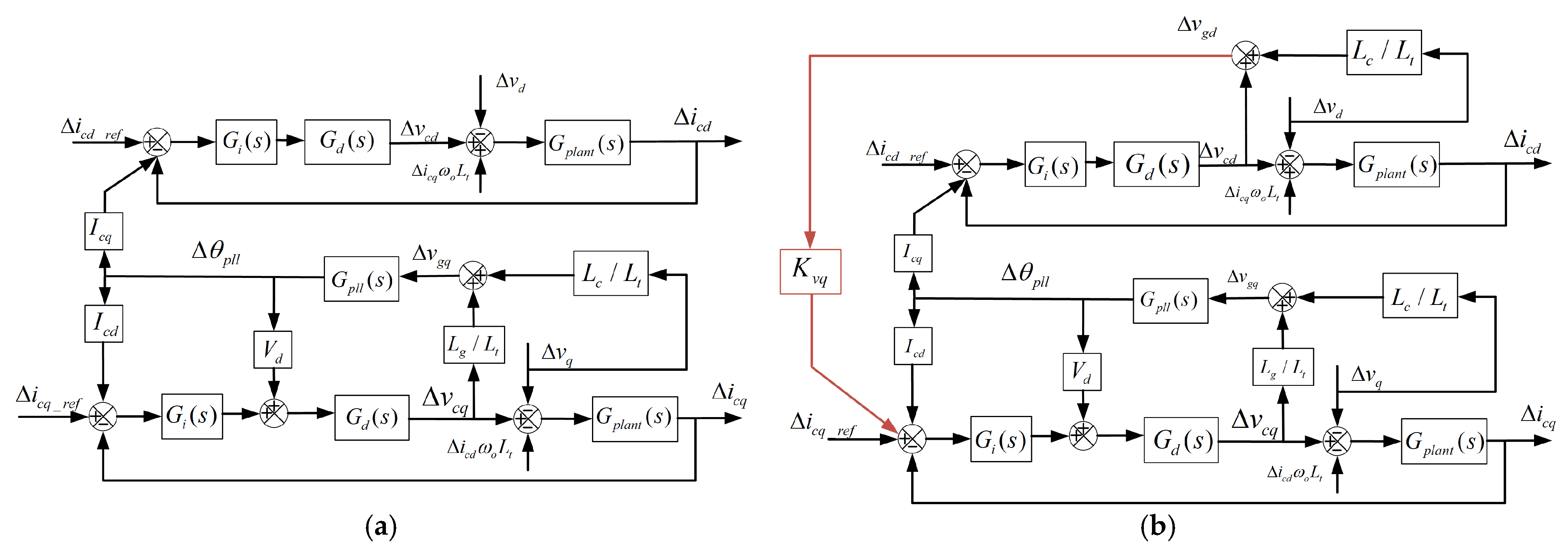
3.1. Derivation of the Small-Signal Control Block Diagram

According to Figure 1, the mathematical model of the STATCOM-side main circuit in the $abc$-coordinate system can be expressed as

$$\begin{array}{c}{v}_{ca}^s\left(t\right)=v_{ga}^s\left(t\right)+L_c{\displaystyle \frac{d{i}_{ca}^s\left(t\right)}{dt}}=v_a^s\left(\mathrm{t}\right)+\left(L_c+L_g\right){\displaystyle \frac{d{i}_{ca}^s\left(t\right)}{dt}}\\ v_{cb}^s\left(t\right)=v_{gb}^s\left(t\right)+L_c{\displaystyle \frac{d{i}_{cb}^s\left(t\right)}{dt}}=v_b^s\left(\mathrm{t}\right)+\left(L_c+L_g\right){\displaystyle \frac{d{i}_{cb}^s\left(t\right)}{dt}}\\ v_{cc}^s\left(t\right)= v_{gc}^s\left(t\right)+L_c{\displaystyle \frac{d{i}_{cc}^s\left(t\right)}{dt}}=v_c^s\left(\mathrm{t}\right)+\left(L_c+L_g\right){\displaystyle \frac{d{i}_{cc}^s\left(t\right)}{dt}}\end{array}$$

(3)

By transforming the above equation into the $dq$-coordinate system, the following can be obtained:

$$\begin{array}{c}{v}_{cd}^s\left(t\right)=v_d^s\left(t\right)+\left(L_c+L_g\right){\displaystyle \frac{d{i}_{cd}^s\left(t\right)}{dt}}-\omega \left(L_c+L_g\right)i_{cd}^s\left(t\right)\\ v_{cq}^s\left(t\right)=v_q^s\left(t\right)+\left(L_c+L_g\right){\displaystyle \frac{d{i}_{cq}^s\left(t\right)}{dt}}-\omega \left(L_c+L_g\right)i_{cq}^s\left(t\right)\end{array}$$

(4)

The above equation is transformed from the time domain to the frequency domain using the Laplace transform, and then small-signal linearization processing is carried out to obtain

$$\begin{array}{c}\left[\Delta v_{cd}\left(s\right)-\Delta v_c\left(s\right)+\Delta i_{cq}\left(s\right){\omega }_0{L}_t\right]G_{plant}\left(s\right)=\Delta i_{cd}\left(s\right)\\ \left[\Delta v_{cq}\left(s\right)-\Delta v_q\left(s\right)-\Delta i_{cd}\left(s\right){\omega }_0{L}_t\right]G_{plant}\left(s\right)=\Delta i_{cq}\left(s\right)\end{array}$$

(5)

where $L_t$ and $G_{plant}\left(s\right)$ are, respectively,

$$L_t=L_c+L_g$$

(6)

$$G_{plant}\left(s\right)={\displaystyle \frac{1}{L_{t}s}}$$

(7)

It can be observed that two cross-coupling terms ($\Delta i_{cq}\left(s\right){\omega }_0{L}_t$ and $-\Delta i_{cd}\left(s\right){\omega }_0{L}_t$) emerge here. This phenomenon arises because the inductances $L_c$ and $L_g$ induce a 90° phase lag between current and voltage, while the orthogonal configuration of the dq axes (also separated by 90°) ensures that the $abc$-to-dq coordinate transformation reflects this inductive characteristic into the dq coordinate system. Consequently, the cross-coupling terms $\Delta i_{cq}\left(s\right){\omega }_0{L}_t$ and $-\Delta i_{cd}\left(s\right){\omega }_0{L}_t$ are introduced, whose presence significantly complicates the subsequent derivation of the system transfer function.

Therefore, the STATCOM state–space model considering grid impedance effects can be obtained as shown in Figure 2a. Here, $\Delta i_{cd}\left(s\right)$ and $\Delta i_{cq}\left(s\right)$ represent the d axis and q axis components of the small-signal perturbations in the STATCOM output current, respectively, $\Delta i_{cd\_ref}\left(s\right)$ and $\Delta i_{cq\_ref}\left(s\right)$ denote the d axis and q axis components of the small-signal perturbations in the STATCOM reference current, respectively; $I_{cd}$ and $I_{cq}$ are the d axis and q axis components of the steady-state STATCOM output current, respectively, $\Delta v_{gd}\left(s\right)$ and $\Delta v_{gq}\left(s\right)$ correspond to the d axis and q axis components of the small-signal perturbations in the PCC voltage, respectively. $\Delta {\theta }_{pll}$ denotes the disturbance quantity in the output voltage of the phase-locked loop. The current controller is denoted by $G_i\left(s\right)$, whilst $G_d\left(s\right)$ represents the linearized control delay [39]. $G_{pll}\left(s\right)$ represents the transfer function of the $\Delta v_{gq}$ to $\Delta {\theta }_{pll}\left(s\right)$ [40], which is expressed as

$$G_{PLL}\left(s\right)={\displaystyle \frac{\Delta {\theta }_{pll}}{\Delta v_{gq}^s}}={\displaystyle \frac{K_{pll\_p}s+K_{pll\_i}}{s^2+V_{gd}^s{K}_{pll\_p}s+K_{pll\_i}}}$$

(8)

3.2. Derivation of the Transfer Function

The system transfer function is derived from Figure 2 with the following considerations. As the STATCOM primarily compensates reactive power, the $d$ axis reference current $\Delta i_{cd\_ref}\left(s\right)$ is designed as zero, resulting in zero steady-state d axis current $I_{cd}$. Under this configuration, the STATCOM maintains phase alignment with the PCC voltage while exclusively exchanging reactive power with the grid.

Furthermore, $\Delta v_{abc}\left(s\right)$ represents ideal sinusoidal voltages, allowing the small-signal perturbations $\Delta v_d\left(s\right)$ and $\Delta v_q\left(s\right)$ to be neglected ($\Delta v_d\left(s\right)=\Delta v_q\left(s\right)=0$). With these assumptions, the system features two control inputs ($\Delta i_{cd\_ref}\left(s\right)$ and $\Delta i_{cq\_ref}\left(s\right)$) and corresponding outputs ($\Delta i_{cd}\left(s\right)$ and $\Delta i_{cq}\left(s\right)$). System stability is evaluated through the transfer matrix expressed as

$$\left[\begin{array}{c}\Delta i_{cd}\left(s\right)\\ \Delta i_{cq}\left(s\right)\end{array}\right]=\left[\begin{array}{cc}{G}_{icd\_cl}\left(s\right)& G_{icqref\_icd}\left(s\right)\\ G_{icdref\_icd}\left(s\right)& G_{icq\_cl}\left(s\right)\end{array}\right]\left[\begin{array}{c}\Delta i_{cd\_ref}\left(s\right)\\ \Delta i_{cq\_ref}\left(s\right)\end{array}\right]$$

(9)

For this system, the system is stable only when the four transfer functions in Equation (10) all have stable poles. Since the droop control focused on in this paper mainly affects the q axis current, the following analysis focuses on the closed-loop transfer function $G_{icq\_cl}\left(s\right)$ from $\Delta i_{cq\_ref}\left(s\right)$ to $\Delta i_{cq}\left(s\right)$.

The control block diagram in Figure 2a without droop control can be simplified through derivation into the control block diagram in Figure 3 that only contains the q axis part.

Firstly, simplify the positive feedback loop passing through $V_d$ that is not coupled with the d axis.

$$G_{q\_pll}\left(s\right)={\displaystyle \frac{L_t{G}_d\left(s\right)}{L_t-L_g{V}_d{G}_d\left(s\right)G_{pll}\left(s\right)}}$$

(10)

Then, it can be seen in Figure 2a that the output signal $\Delta i_{cd}\left(s\right)$ of the d axis has an impact on the q axis through the coupling term $-\Delta i_{cd}\left(s\right){\omega }_0{L}_t$, and $\Delta i_{cd}\left(s\right)$ can be expressed as

$$\Delta i_{cd}\left(s\right)=G_{vcq\_icd}\left(s\right)\Delta v_{cq}+G_{icq\_icd}\left(s\right)\Delta i_{cq}$$

(11)

$G_{vcq\_icd}\left(s\right)$ denotes the transfer functions from $\Delta v_{cq}$ to $\Delta i_{cd}$ and $G_{icq\_icd}\left(s\right)$ denotes the transfer functions from $\Delta i_{cq}$ to $\Delta i_{cd}$. They can be derived as

$$G_{vcq\_icd}\left(s\right)={\displaystyle \frac{L_g{I}_{cq}{G}_{pll}\left(s\right)G_i\left(\mathrm{s}\right)G_d\left(\mathrm{s}\right)G_{plant}\left(\mathrm{s}\right)}{L_t+L_t{G}_i\left(\mathrm{s}\right)G_d\left(\mathrm{s}\right)G_{plant}\left(\mathrm{s}\right)}}$$

(12)

$$G_{icq\_icd}\left(s\right)={\displaystyle \frac{{\omega }_0{L}_t{G}_{plant}\left(\mathrm{s}\right)}{1+G_i\left(\mathrm{s}\right)G_d\left(\mathrm{s}\right)G_{plant}\left(\mathrm{s}\right)}}$$

(13)

Now, from Figure 3, the closed-loop transfer function $G_{icq\_cl}\left(s\right)$ on the $q$ axis can be obtained.

$$G_{icq\_cl}\left(s\right)={\displaystyle \frac{G_i\left(s\right)G_{q\_pll}\left(s\right)G_{vcq\_icq}\left(s\right)}{1+G_i\left(s\right)G_{q\_pll}\left(s\right)G_{vcq\_icq}\left(s\right)}}$$

(14)

Among them, $G_{vcq\_icq}\left(s\right)$ is the transfer function from $\Delta v_{cq}$ to $\Delta i_{cq}$:

$$G_{vcq\_icq}\left(s\right)={\displaystyle \frac{G_{plant}\left(s\right)-{\omega }_0{L}_t{G}_{plant}\left(s\right)G_{vcq\_icd}\left(s\right)}{1+{\omega }_0{L}_t{G}_{icq\_icd}\left(s\right)G_{plant}\left(s\right)}}$$

(15)

Subsequently, droop control is incorporated into the control system. As shown in Figure 4, the application of droop control is manifested as the red signal line that connects $\Delta v_{gd}$ to the $q$ axis on the control block diagram. Since this paper primarily focuses on the stability of the transfer functions in Equation (9) and assumes that the grid voltage is stable, $\Delta v_d$ and $\Delta v_q$ are equal to 0. To obtain the expression of $\Delta v_{gd}$, the same approach as described above is adopted.

$$\Delta v_{gd}\left(s\right)=G_{vcq\_vgd}\left(s\right)\Delta v_{cq}+G_{icq\_vgd}\left(s\right)\Delta i_{cq}$$

(16)

$G_{vcq\_vgd}\left(s\right)$ denotes the transfer functions from $\Delta v_{cq}$ to $\Delta v_{gd}$ and $G_{icq\_vgd}\left(s\right)$ denotes the transfer functions from $\Delta i_{cq}$ to $\Delta v_{gd}$. They can be derived as

$$G_{icq\_vgd}\left(s\right)={\displaystyle \frac{{\omega }_0{L}_g{G}_i\left(\mathrm{s}\right)G_d\left(\mathrm{s}\right)G_{plant}\left(\mathrm{s}\right)}{1+G_i\left(\mathrm{s}\right)G_d\left(\mathrm{s}\right)G_{plant}\left(\mathrm{s}\right)}}$$

(17)

$$G_{vcq\_vgd}\left(s\right)={\displaystyle \frac{L_g^2{G}_i\left(\mathrm{s}\right)G_d\left(\mathrm{s}\right)G_{pll}\left(\mathrm{s}\right)}{L_t^2+L_t^2{G}_i\left(\mathrm{s}\right)G_d\left(\mathrm{s}\right)G_{plant}\left(\mathrm{s}\right)}}$$

(18)

In the previous subsection, by deriving the expression of $G_{vcq\_icq}\left(s\right)$, the forward path in the control block diagram has become extremely concise. As shown in Figure 4, the two new paths introduced due to the droop control have complicated the feedback path. First, the feedback path is simplified. Let $G_{icq\_icqref}\left(s\right)$ represent the feedback path from $\Delta i_{cq}$ to $\Delta i_{cq\_ref}$.

$$G_{icq\_icqref}\left(s\right)={\displaystyle \frac{G_{vcq\_icq}\left(s\right)-K_{vq}{G}_{vcq\_vgd}\left(s\right)-K_{vq}{G}_{icq\_vgd}\left(s\right)G_{vcq\_icq}\left(s\right)}{G_{vcq\_icq}\left(s\right)}}$$

(19)

The concise closed-loop transfer function of the $q$ axis after adding the droop control can be derived.

$$G_{icq\_cl\_dr}\left(s\right)={\displaystyle \frac{G_i\left(s\right)G_{q\_pll}\left(s\right)G_{vcq\_icq}\left(s\right)}{1+G_{icq\_icqref}\left(s\right)G_i\left(s\right)G_{q\_pll}\left(s\right)G_{vcq\_icq}\left(s\right)}}$$

(20)

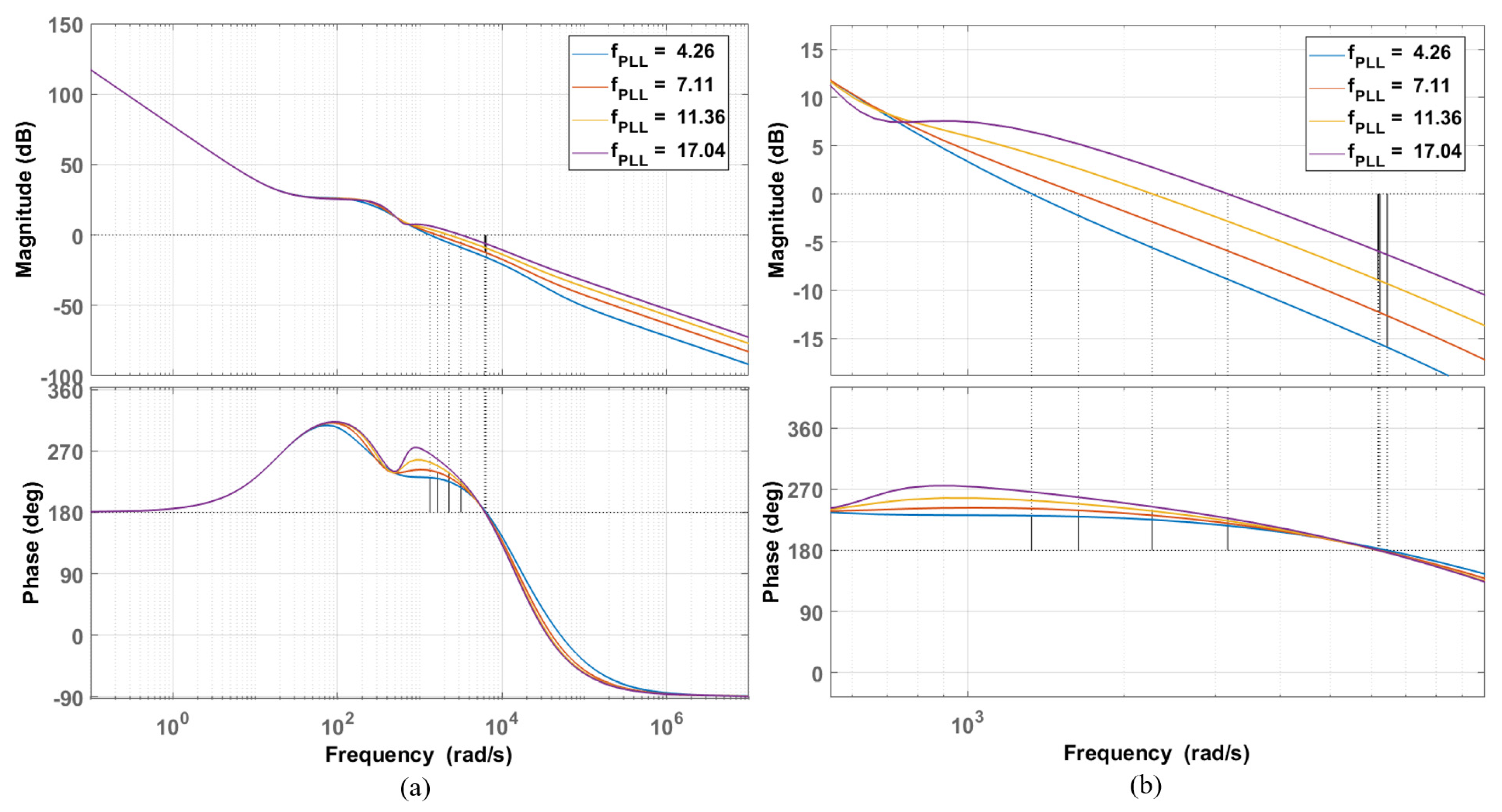
3.3. Stability Analysis

First and foremost, it is crucial to clarify the modifications induced by the incorporation of droop control into the system. The comparative analysis of Figure 3 and Figure 4 reveals that the implementation of droop control essentially introduces a positive feedback loop whose gain is regulated by the droop control coefficient $K_{vq}$. To quantitatively demonstrate the impact of this feedback path on system, Figure 5 presents the Bode diagrams of the system’s open-loop transfer function under varying $K_{vq}$ values.

When $K_{vq}$ is set to zero, the system exhibits substantial gain margin and phase margin. Upon the implementation of droop control, both gain and phase margins experience significant reduction, leading to the deterioration of system stability. When $K_{vq}$ is increased to 2, both margins become negative, resulting in system instability. The specific gain and phase margins corresponding to different $K_{vq}$ values are tabulated below. Under the system parameters listed in

Table 1. Gain and phase margin analysis under different $K_{vq}$ values.

${\mathit{K}}_{\mathit{v}\mathit{q}}$	Gain Margin/dB	Phase Margin/Deg
0	22	69
0.5	9.44	50.7
1	3.94	26.9
1.6	0.0443	0.353
1.7	−0.464	−3.76
1.8	−0.944	−7.8
2	−1.83	−15.6

, the critical stability threshold occurs at approximately $K_{vq}=1.6$.

A closer examination of Figure 4 reveals that the droop control introduces two transfer functions, denoted as $G_{vcq\_vgd}\left(s\right)$ and $G_{icq\_vgd}\left(s\right)$, which are mathematically defined by Equations (18) and (19), respectively. Both functions incorporate the grid inductance parameter $L_g$ and exhibit proportionality to $L_g$. This relationship explicitly elucidates the mechanism through which the droop control method interacts with grid impedance, with such an interaction directly contributing to stability challenges. When $L_g=0 \mathrm{mH}$, corresponding to a strong grid condition, both $G_{vcq\_vgd}\left(s\right)$ and $G_{icq\_vgd}\left(s\right)$ become zero, rendering the droop control entirely ineffective in modifying the system transfer function. As previously discussed, this droop control strategy becomes unnecessary for grid voltage support under non-weak grid conditions. Figure 6 quantitatively demonstrates the impact of $L_g$ on system stability, where increased $L_g$ values correlate with heightened instability risks. These observations underscore the necessity for developing stability-enhancing methodologies tailored for droop-controlled systems operating in weak grid environments.

4. Virtual Inductance Control

This section introduces the virtual control method we proposed. The first section demonstrates the control method proposed in this paper through formula derivation, and the second section analyzes the specific impact of this control method on the stability of the system.

4.1. Formula Derivation

As discussed earlier, $K_{vq}$ and $L_g/L_t$ have a significant impact on the stability of STATCOM with droop control in a weak grid, and the method proposed in this paper is precisely based on this point. A straightforward approach is to reduce $L_g/L_t$. Since altering the grid impedance is impractical, the only factor that can be changed is $L_c$. If an actual inductor $L_d$ is inserted between the PCC and the filter inductor $L_c$, as shown in Figure 7, it is equivalent to increasing the filter inductor $L_c$ and reducing $L_g/L_t$, thus reducing the impact of the droop control loop on the stability of STATCOM.

At this time, $G_{plant}\left(\mathrm{s}\right)$ can be rewritten as

$$G_{plant\_d}\left(s\right)={\displaystyle \frac{1}{L_{t}s+L_{d}s}}$$

(21)

Continuing the analysis, the pole-zero map of $G_{icq\_cl\_dr}\left(s\right)$ is plotted, as shown in Figure 8. As seen in Figure 8, as $L_d$ increases, the unstable poles initially in the right half-plane move to the left, and the system transitions from unstable to stable.

However, modifying the circuit is not an ideal option due to the characteristics of actual inductors, such as their large volume and high cost. Moreover, in practice, it is difficult to determine the precise and stable grid impedance $L_g$ in advance. Consequently, selecting an appropriate $L_d$ for installation is also not feasible. Therefore, this paper proposes a control strategy for virtual inductors. The control block diagram in Figure 9 illustrates the derivation process of the d axis. The same principle applies to the q axis, and thus further discussion is omitted.

The control block diagram with the addition of an actual inductor is shown in Figure 9a. Note that the system impedance in the diagram is $G_{plant\_d}\left(s\right)$. The transfer function from $\Delta i_{cd\_ref}$ to $\Delta i_{cd}$ is given by

$${\displaystyle \frac{\Delta i_{cd}}{\Delta i_{cd\_ref}}}={\displaystyle \frac{G_i\left(s\right)G_d\left(s\right)G_{plant\_d}\left(s\right)}{1+G_i\left(s\right)G_d\left(s\right)G_{plant\_d}\left(s\right)}}$$

(22)

The method proposed in this paper does not alter the circuit topology; hence, the system impedance remains $G_{plant}\left(s\right)$. Consequently, the control part is modified to achieve the same effect as an actual inductor. First, a new feedback loop is added to the original control system, as shown in Figure 9b. Thus, the transfer function from $\Delta i_{cd\_ref}$ to $\Delta i_{cd}$ is given by

$${\displaystyle \frac{\Delta i_{cd}}{\Delta i_{cd\_ref}}}={\displaystyle \frac{G_i\left(s\right)G_d\left(s\right)G_{plant}\left(s\right)}{1+G_i\left(s\right)G_d\left(s\right)G_{plant}\left(s\right)H\left(s\right)}}$$

(23)

In order to make the effect of the added feedback loop consistent with that of the actual inductor, let Equation (22) be equal to Equation (23), that is

$${\displaystyle \frac{G_i\left(s\right)G_d\left(s\right)G_{plant\_d}\left(s\right)}{1+G_i\left(s\right)G_d\left(s\right)G_{plant\_d}\left(s\right)}}={\displaystyle \frac{G_i\left(s\right)G_d\left(s\right)G_{plant}\left(s\right)}{1+G_i\left(s\right)G_d\left(s\right)G_{plant}\left(s\right)H\left(s\right)}}$$

(24)

Solving (24), $H\left(s\right)$ is derived as

$$H\left(s\right)=1+{\displaystyle \frac{L_{d}s}{G_i\left(s\right)G_d\left(s\right)}}$$

(25)

Given that the control system already includes a negative feedback loop, $H\left(s\right)$ can be divided into two parts, using the plus sign in Equation (25) as the boundary. The first part represents the original negative feedback, while the second part represents the equivalent of the actual inductor. Subsequently, the comparison point is shifted backward. The control system block diagram is shown in Figure 9c, and $G_{vi}\left(s\right)$ therein is

$$G_{vi}\left(s\right)=-L_{d}s$$

(26)

Equation (26) contains an integral term, and implementing this term in the controller is challenging. Given that the feedback loop is derived from $\Delta i_{cd}$, the relationship between $\Delta i_{cd}$ and the voltage drop across the inductor is employed to eliminate the integral term. It can be expressed as follows:

$$\Delta i_{cd}={\displaystyle \frac{\Delta v_{cd}-\Delta v_d}{\left(L_t+L_d\right)s}}$$

(27)

Now the integral term in $G_{vi}\left(s\right)$ can be eliminated:

$$\Delta i_{cd}{G}_{vi}\left(s\right)=\left(\Delta v_d-\Delta v_{cd}\right){\displaystyle \frac{L_d}{L_t+L_d}}$$

(28)

The virtual inductance coefficient $K_{vi}$ is defined as

$$K_{vi}={\displaystyle \frac{L_d}{L_t+L_d}}$$

(29)

The final control scheme is shown in Figure 9d. By tuning $K_{vi}$, the system impedance can be adjusted. Without altering the circuit topology, the impedance ratio $L_g/L_t$ is reduced, thereby reducing the impact of droop control on system stability in weak grid conditions.

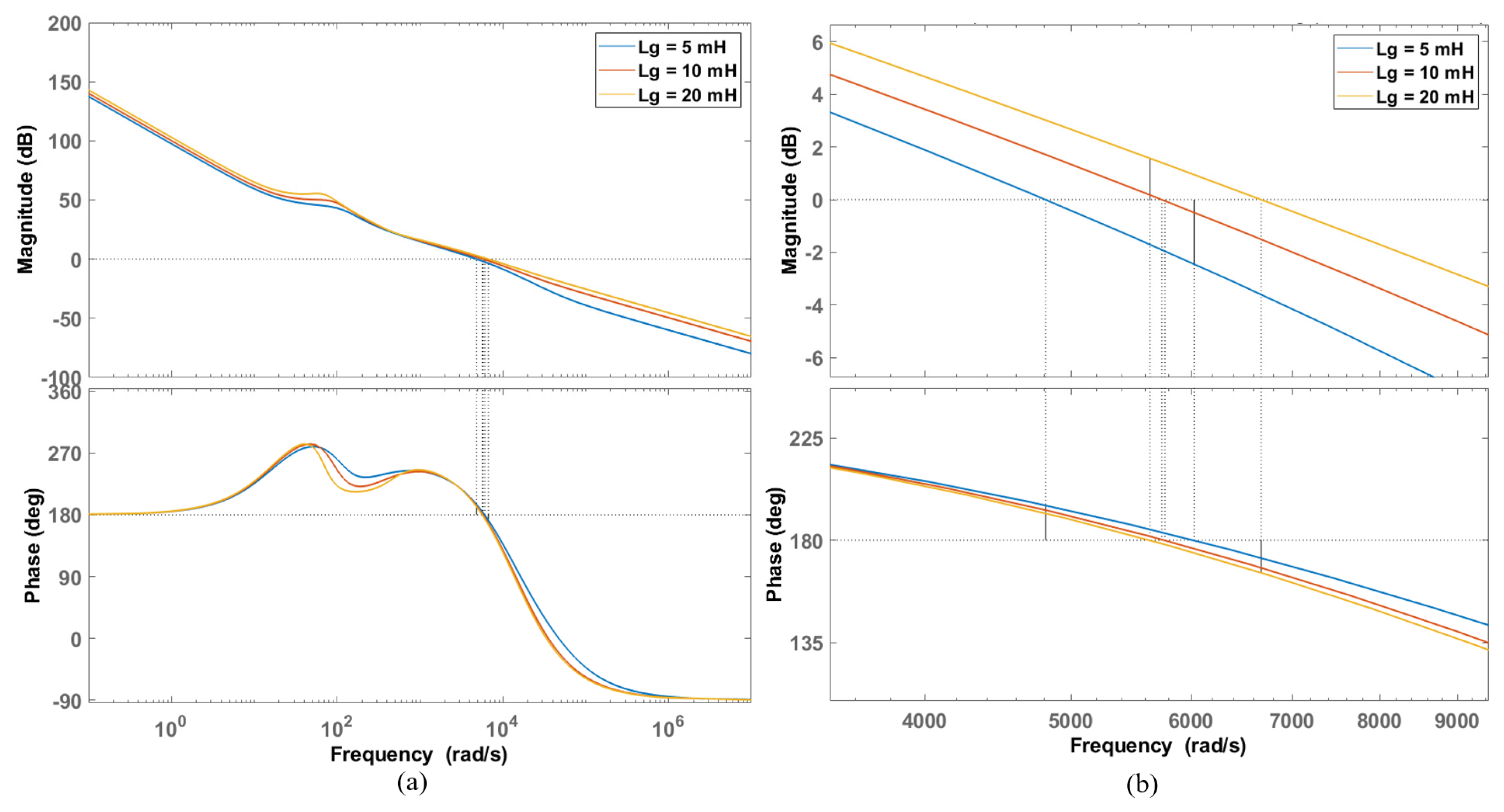
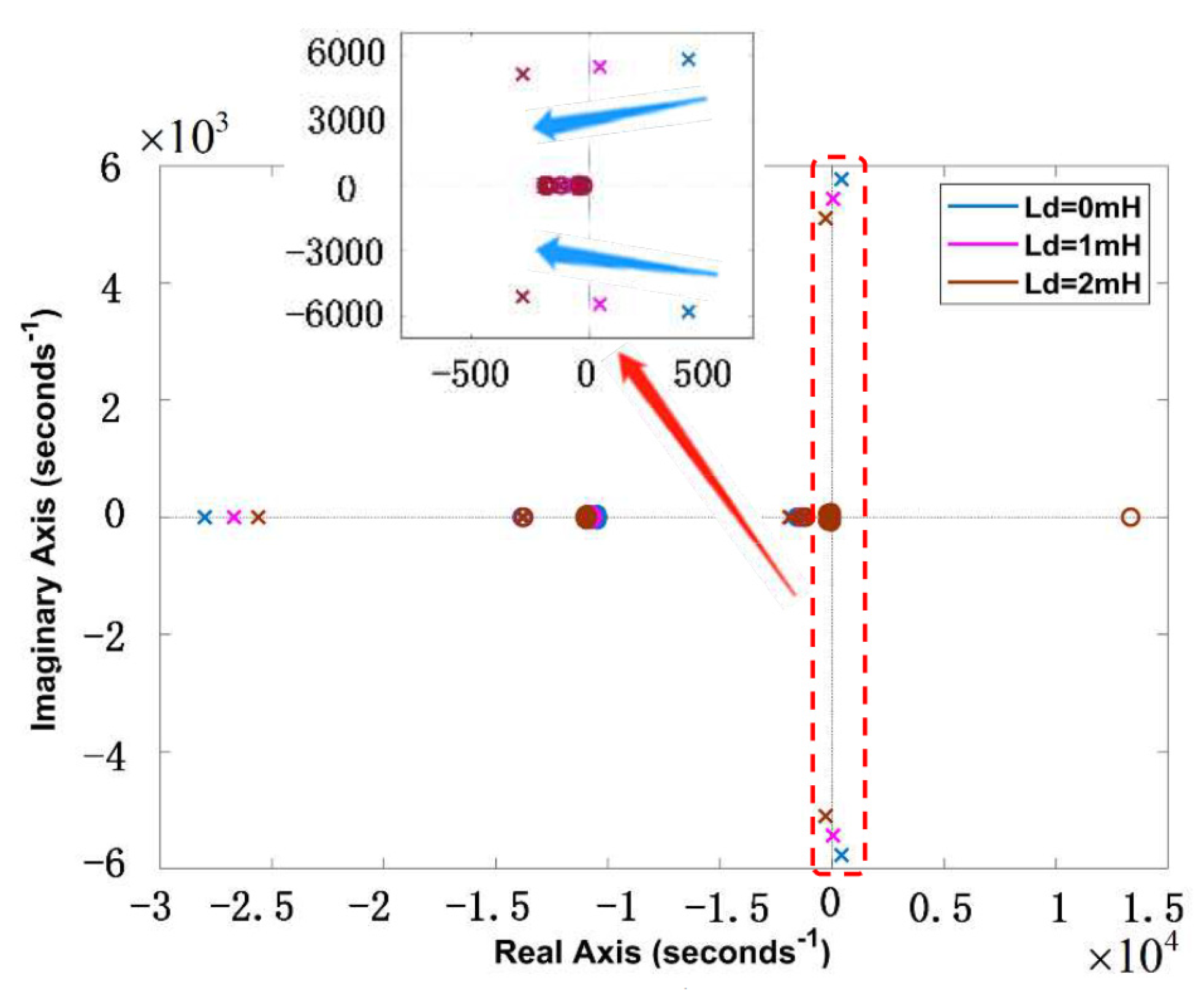
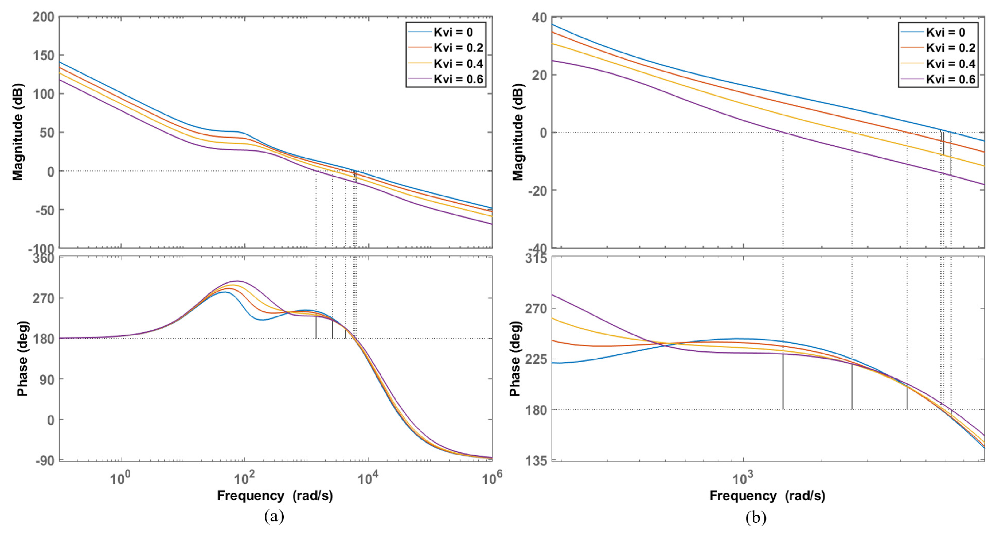
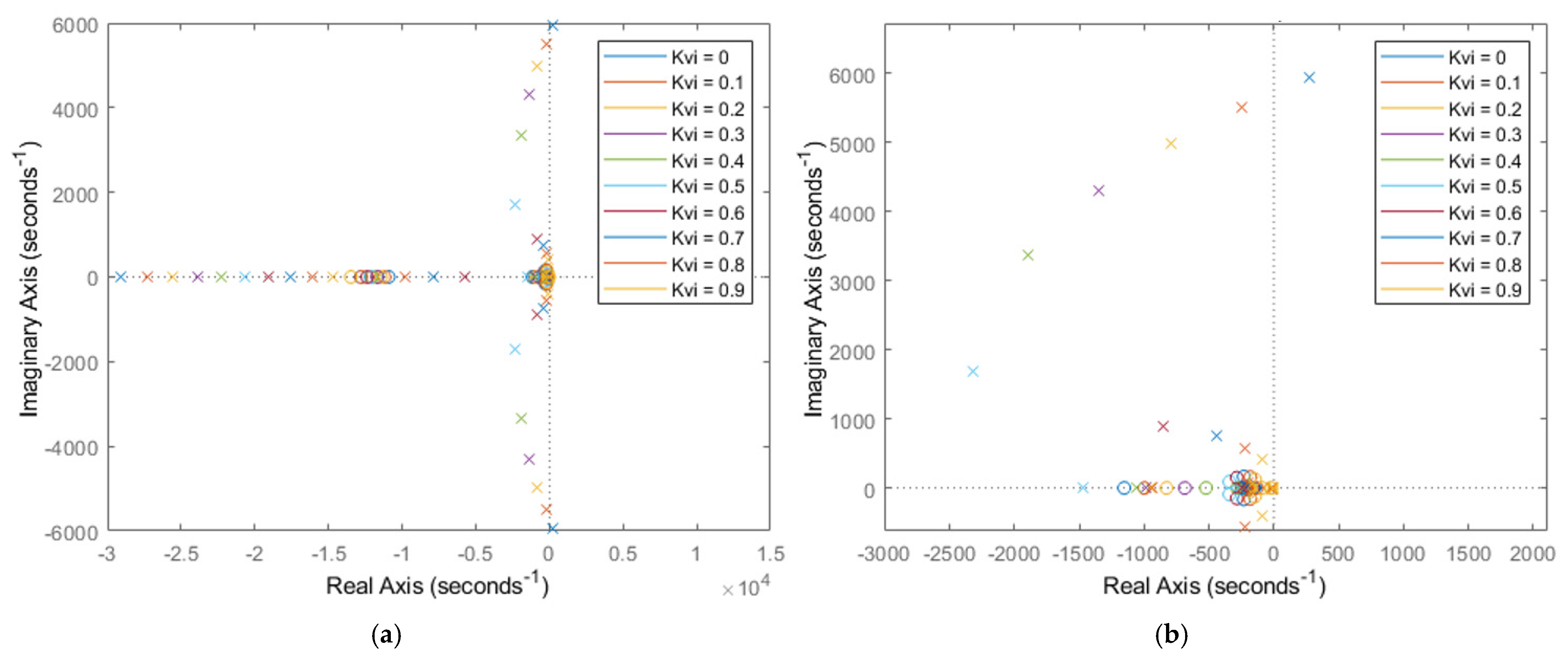
4.2. Stability Analysis

The following addresses the selection of virtual inductance coefficients. Figure 10 demonstrates the Bode plot variations of the system’s open loop transfer function with different $K_{vi}$ values.

As evident from the results, increasing $K_{vi}$ induces a system transition from instability to stability, accompanied by progressive enhancements in both gain margin and phase margin, indicating improved system robustness. However, this does not imply the monotonic superiority of elevated $K_{vi}$ values. Figure 11 illustrates the corresponding variations in the pole-zero configuration of the closed-loop transfer function with ascending $K_{vi}$.

The system exhibits a dominant pole pair, from whose positions the approximate damping ratio $\zeta$ can be derived as demonstrated in Figure 12.

The calculated $\zeta$ displays an initial increase followed by a decrease, with two instances attaining the optimal damping ratio of 0.707. Control theory establishes that dominant poles positioned farther from the origin correspond to accelerated transient response (reduced settling time) at the expense of degraded high-frequency noise immunity. Given the critical sensitivity to high-frequency disturbances inherent in power electronic systems, the design prioritizes enhanced robustness by selecting $K_{vi}=0.59$, which maintains the dominant poles at appropriately distant locations from the origin.

Figure 10 demonstrates that the introduction of virtual impedance reduces the system bandwidth, consequently impairing dynamic response performance. As indicated by Equation (9), PLL parameters constitute another critical factor affecting system performance, where PLL bandwidth significantly influences the dynamic response characteristics. Figure 13 illustrates the impact of PLL bandwidth ($f_{PLL}$) on system performance under virtual inductance implementation. The influences on the amplitude margin and phase Angle margin are presented in

Table 2. Gain and phase margin analysis under different $f_{\mathit{PLL}}$ values.

${\mathit{f}}_{\mathit{P}\mathit{L}\mathit{L}}$	Gain Margin/dB	Phase Margin/Deg
4.26	15.9	51.1
7.11	12.3	58.9
11.36	8.92	58
17.04	5.96	47.3

. The results show that increasing the PLL bandwidth enhances the system bandwidth while maintaining stability, thereby improving dynamic response capability.

5. Simulation and Experimental Results

This section is the simulation and experimental verification of the control method proposed in this paper. The first section demonstrates the effectiveness of this control method by comparing it with the traditional power control. The second section demonstrates its practical effect through an actual inverter.

5.1. Simulation

To validate the effectiveness of the proposed methodology, two simulation models were developed in MATLAB 2021a/Simulink: the proposed method and a conventional power-controlled STATCOM [35] for comparative analysis.

5.1.1. Parameter Description

For the method we propose, the corresponding control and system parameters are shown in

Table 3. Main system parameters and control parameters.

Symbol	Description	Value
Vdc	DC-link voltage	500 V
Lc	Filter inductance	4 mH
Vgd	Grid voltage amplitude	100 V
Lg	Grid inductance	10 mH
fs	Sampling/switching frequency	10 KHz
Kpll_p	PLL proportional gain	3
Kpll_i	PLL integral gain	300
Kcp	Current regulator proportional gain	15
Kci	Current regulator integral gain	300
Icd_ref	Current reference of d axis	0 A
Icq_ref	Current reference of q axis	5 A

. Hardware parameters are maintained consistent with laboratory equipment specifications. The grid voltage amplitude is configured at an unconventional 100 V value due to the experimental constraints imposed by the maximum power capacity of the experimental apparatus, which preclude experimentation at standard voltage levels. Control parameters are optimized through multiple iterative refinement processes. Reference current values are determined based on comprehensive safety assessments of the experimental system.

The system and control parameters employed in the comparative model are detailed in

Table 4. System and control parameters of the comparative model.

Symbol	Description	Value
Vdc	DC-link voltage	500 V
Lc	Filter inductance	4 mH
Vgd	Grid voltage amplitude	100 V
Lg	Grid inductance	10 mH
fs	Sampling/switching frequency	10 KHz
kpPLL	PLL proportional gain	3
kiPLL	PLL integral gain	300
kpi	Current controller proportional gain	15
kii	Current controller integral gain	300
kpac	AC voltage controller proportional gain	0.01
kiac	AC voltage controller integral gain	5
kpdc	DC voltage controller proportional gain	1.25
kidc	DC voltage controller integral gain	0.225
Qref	Current reference of d axis	500 W
Vdc_ref	Current reference of q axis	500 V

.

5.1.2. Analysis of SCR in the System

As can be seen from Table 3, the weak grid in this paper is approximated by an ideal voltage source with an inductor. This approximation method is chosen because the grid impedance of long-distance transmission lines generally exhibits resistive–inductive characteristics. It is well known that resistive impedance contributes to stability enhancement. However, to demonstrate the effectiveness of the proposed control method under harsh conditions, this paper approximates the grid impedance as purely inductive. Notably, this approximation has been widely adopted [29,41].

The introduction of this paper states that a system can be considered a weak grid when its SCR is less than 3. To justify the selection of the grid inductance value, the system’s SCR is calculated as follows:

$$SCR={\displaystyle \frac{I_{sc}}{I_{rated}}}={\displaystyle \frac{V_{gd}}{\sqrt{3}{X}_{grid}{I}_{rated}}}={\displaystyle \frac{V_{gd}}{\sqrt{3}·2\pi f{L}_g{I}_{rated}}}=2.62$$

(30)

Here, $I_{sc}$ represents the short-circuit current, $I_{rated}$ represents the rated current, and $X_{grid}$ represents the grid reactance. $I_{rated}$ is equal to $I_{cq\_ref}$.

The calculations demonstrate that our approximation method complies with IEEE standard 1204-1997. However, it should be noted that this approximation inevitably differs from real weak grid conditions, where the actual grid impedance comprises a combination of resistance, inductance, and capacitance. Nevertheless, this paper argues that the impact of this widely adopted approximation on the stability issues under investigation is negligible.

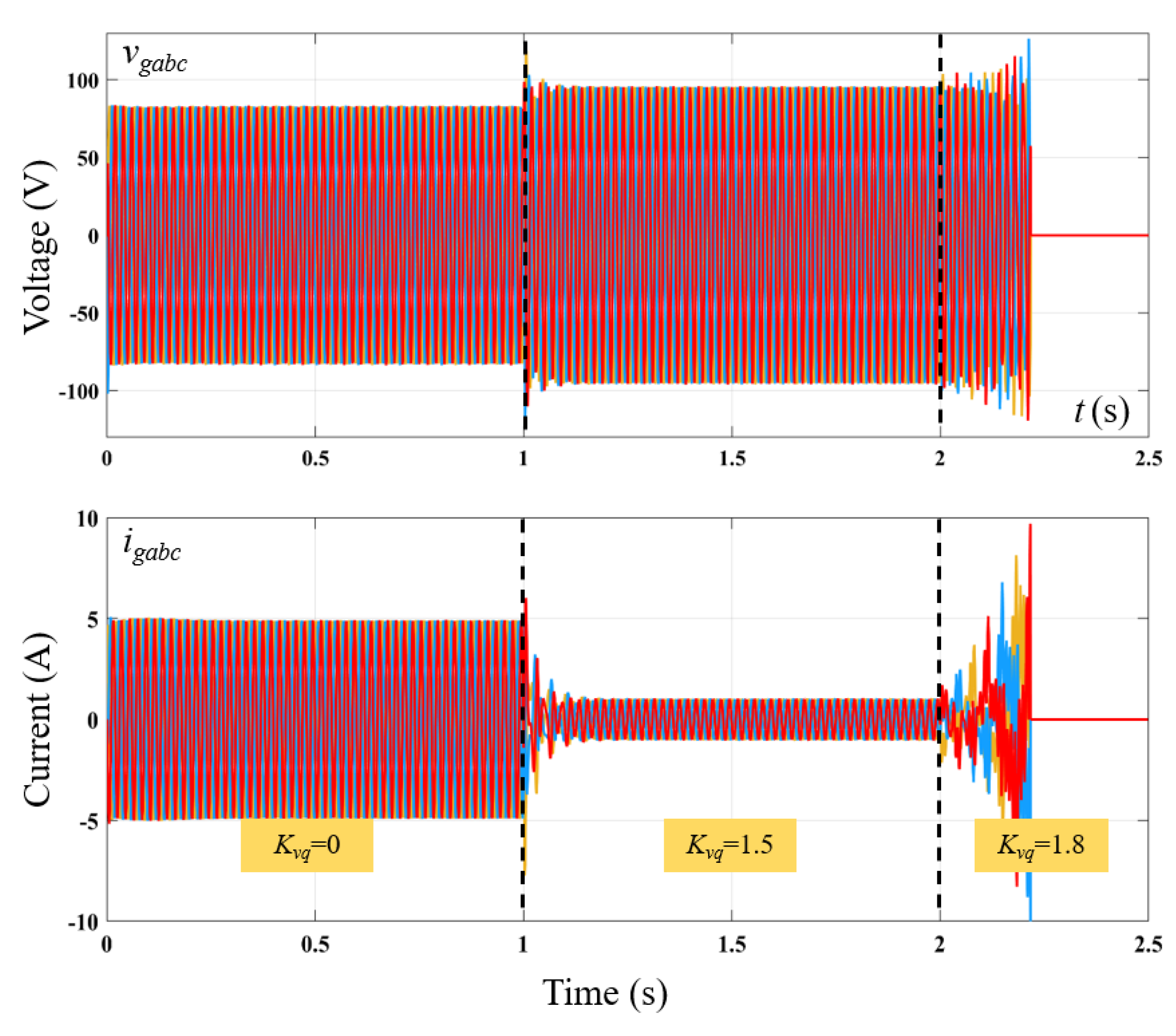
5.1.3. Stability Validation

Figure 14 presents the waveforms of the voltage at the PCC and the output current of the STATCOM under a weak grid as the voltage droop control coefficient changes. To analyze the dynamic changes of the STATCOM grid-connected system more clearly, the waveform of the voltage at the PCC, $v_{gabc}$ is filtered. Before $t=1 \mathrm{s}$, the droop control is not added to the system. At this time, the amplitude of the voltage at the grid-connected point $v_{gabc}$ is only 82.5 V, which is significantly lower than the set value of 100 V for the system. This phenomenon is mainly caused by the fact that the STATCOM is operating in an environment where the grid strength is relatively weak and the supporting capacity of the grid itself is insufficient.

At $t=1 \mathrm{s}$, the voltage droop control with $K_{vq}=1.5$ is implemented. The amplitude of the voltage at the PCC increases significantly, effectively mitigating the voltage drop issue due to the weak grid. During this process, the STATCOM rapidly supplies reactive power to meet the system’s reactive power demand, thereby raising the grid-connected voltage amplitude. Concurrently, as the reactive power in the STATCOM is consumed, the output current decreases from 5 A to 1 A, and the grid-connected voltage amplitude reaches 96.2 V.

At $t=2 \mathrm{s}$, the voltage droop coefficient $K_{vq}$ is increased to 1.8. Subsequently, as time progresses, the amplitude of the output current $i_{cabc}$ continues to increase and exhibits a trend of unbounded growth. It eventually exceeds the system’s maximum output limit, activating the system protection mechanism and halting system operation.

The simulation results confirm that STATCOM can effectively compensate for the reactive power required by the system in a weak grid and regulate the voltage at the PCC. However, setting the voltage droop coefficient too high can cause a sharp increase in current and degrade the system performance, activating the system’s security protection mechanism. Additionally, this result suggests that the coupling effect between STATCOM’s voltage droop control and grid inductance can indeed cause the system to become unstable.

Figure 15 shows the waveform variations of the voltage at the PCC ($v_{gabc}$) and the output current of the STATCOM ($i_{cabc}$) before and after adding virtual impedance control to the STATCOM grid-connected system. By comparing with the results after removing the virtual impedance control ($K_{vi}=0.59$), it is evident that, upon introducing the virtual impedance control into the STATCOM with the droop coefficient $K_{vq}=1.8$, the three-phase waveforms of the voltage at the PCC ($v_{gabc}$) and the output current ($i_{gabc}$) remain balanced, the system remains stable, and operates as intended. After removing the virtual inductor, the system becomes unstable and the output current $i_{cabc}$ increases significantly.

The enhancement of stability is achieved at the expense of reduced reactive power support capability. To demonstrate this phenomenon, multiple simulations are conducted by varying $K_{vi}$ values under the condition of $K_{vq}=1.5$ (where the system remains stable without virtual inductance implementation). To further investigate the impact of virtual impedance on dynamic performance, the transient response of reactive power variation caused by the $i_{q\_ref}$ increment is specifically captured, as shown in Figure 16.

As observed in Figure 16, variations in $K_{vi}$ directly influence the system’s output reactive power, with higher $K_{vi}$ values resulting in reduced transmitted reactive power. Moreover, as $K_{vi}$ increases, the system’s overshoot progressively decreases while the settling time is marginally reduced, a trend consistent with the pole-zero migration pattern demonstrated in Figure 12.

5.1.4. Functional Comparison

To demonstrate the functional capabilities and specific performance metrics of the proposed methodology, this section examines the prevalent grid voltage sag scenario—a common power quality disturbance typically induced by short-circuit faults, abrupt load variations, or system contingencies. Comparative evaluations are conducted under simulated grid voltage conditions reduced to 80% of the rated nominal value. Figure 17 compares the dynamic responses of the proposed virtual impedance-integrated methodology and conventional power-regulated STATCOM under grid voltage sag conditions.

Figure 17a,b both demonstrate grid voltage sag conditions in the $v_{abc}$ phase voltages, with amplitude reductions from 100 V to 80 V. However, the system responses exhibit significant divergence due to the distinct control strategies. A comparative analysis of the $v_{gabc}$ waveforms reveals that the proposed methodology inherently provides voltage support: even prior to the voltage sag event, the phase voltage amplitude at the PCC in Figure 17a maintains closer proximity to the rated 100 V nominal value. This discrepancy becomes markedly pronounced post-sag, as evidenced by the synchronous voltage collapse of $v_{gabc}$ in Figure 17b under conventional control.

The current response characteristics exhibit fundamental operational distinctions between the two models. While both systems demonstrate current magnitude elevation, the underlying mechanisms differ substantially. In Figure 17a, the $q$ axis current transitions from approximately 1 A to −4 A, which is indicative of the intentional capacitive reactive power injection required for voltage support functionality. Conversely, Figure 17b manifests current escalation resulting from reactive power reference limitations under grid voltage depression conditions, where the reduced network voltage inherently necessitates an increased current to maintain power transfer requirements.

The following qualitatively examines the system performance metrics following virtual control implementation.

Table 5. System performance metrics under various voltage sag conditions.

$\mathbf{Voltage} \mathbf{Sag} \mathbf{Depth}$	Overshoot	Settling Time/ms
20%	20%	21.7
40%	26%	22.7
60%	34%	23.5
80%	40%	28

details the settling time and overshoot of the $q$ axis current $i_q$ across varying grid voltage sag scenarios.

The simulation results demonstrate that, when STATCOM employs voltage droop control to regulate the voltage at the PCC in a weak grid, the additional loops introduced can degrade system stability, and the virtual inductor control method can improve the system stability under these conditions.

5.2. Experiment

To further validate the effectiveness of the proposed method, a laboratory prototype is developed with a system design consistent with Figure 1 and parameters aligned with Table 3. Figure 18 illustrates the experimental setup. The STATCOM comprises a three-phase inverter and filter inductor. The inverter is controlled by a Texas Instruments TMS320F28379D processor, with sensing, filtering, and IGBT driving functions implemented through dedicated circuit boards. The filter inductor (4 mH) matches the simulation configuration. The source side employs an IT-M3904C bidirectional programmable DC power supply providing 500 V DC. The load side simulates a weak grid using a Chroma 61815 regenerative grid simulator and 10 mH inductor, maintaining consistency with the simulation setup.

Figure 19 and Figure 20 show the STATCOM current waveforms without virtual inductors for varying droop control parameters. Figure 11 shows that, when $K_{vq}=1.5$, the current decreases to provide additional reactive power, maintaining system stability. As shown in Figure 20, when $K_{vq}=1.8$, the output current does not decrease further as in Figure 19. Instead, it increases significantly, indicating system instability. This result aligns with expectations and previous theories and simulations.

After adding the virtual inductor, STATCOM stability is enhanced, as illustrated in Figure 21. With $K_{vq}$ set to 1.8 (as in Figure 20), the system remains stable. However, removing the virtual inductor control method causes the output current to increase significantly and the system to become unstable.

This paper also conducts experiments under grid voltage step-change conditions. To more clearly demonstrate the effectiveness of the proposed method, the grid voltage is subjected to both 40% sag and swell relative to the rated voltage. Figure 22 presents the corresponding system responses. During voltage sag, the phase-a PCC voltage $v_{ga}$ exhibits a minor drop while still providing voltage support. During voltage swell, $v_{ga}$ shows only a slight increase, indicating that the STATCOM effectively suppresses voltage elevation and maintains PCC voltage stability.

While Figure 19 exhibits discernible minor perturbations in experimental current waveforms that deviate from simulation results, these discrepancies are primarily attributed to unmodeled hardware noise in physical implementations. Comparative analysis of Figure 14 and Figure 19 reveals distinct transient responses during droop control activation while achieving equivalent steady-state performance. This divergence likely stems from the continuous-time controller implementation in simulations versus discrete-time execution in the DSP-based digital controller. Nevertheless, the experimental outcomes sufficiently validate the effectiveness of the proposed methodology despite these implementation-dependent variations.

6. Conclusions and Future Work

This paper identifies the root cause for the instability of STATCOMs with voltage-droop support in weak grids. It is shown that the voltage-droop control loop exacerbates the coupling effects between the d axis and the q axis in STATCOMs. These coupling effects become more severe especially in weak grids and thus destabilize the system. To address this issue, a virtual inductor control scheme is proposed to minimize the coupling effects between the d axis and the q axis, thereby improving and enhancing system stability. The proposed method avoids the cost and volume issues associated with adding physical inductance in traditional approaches. It not only improves the operational stability of the STATCOM but also enhances its voltage support capability, thereby supplementing stability research for weak grids with STATCOMs under this specific condition. The effectiveness of the proposed method has been verified in both the simulation model and the laboratory prototype.

Although this paper focuses on a single-machine system, the issue of coupling between droop control loops and grid impedance—which affects stability—also exists in multi-STATCOM systems within weak grids. Therefore, the proposed method has the potential to be extended to multi-STATCOM systems. However, interactions among STATCOMs in such systems may lead to differences in the model compared to the single-machine system. Consequently, multi-STATCOM systems warrant further in-depth analysis and will be the focus of our subsequent research.

As theoretically anticipated, the virtual inductance method not only mitigates droop control-weak grid coupling but also reduces PLL parameter sensitivity, with deeper analyses reserved for future investigations.

References

1. Zeng, Y.; Xiao, Z.; Liu, Q.; Liang, G.; Rodriguez, E.; Zou, G.; Zhang, X.; Pou, J. Physics-Informed Deep Transfer Reinforcement Learning Method for the Input-Series Output-Parallel Dual Active Bridge-Based Auxiliary Power Modules in Electrical Aircraft. IEEE Trans. Transp. Electrif. 2025, 11, 6629–6639. [Google Scholar] [CrossRef]
2. Zeng, Y.; Jiang, S.; Konstantinou, G.; Pou, J.; Zou, G.; Zhang, X. Multi-Objective Controller Design for Grid-Following Converters with Easy Transfer Reinforcement Learning. IEEE Trans. Power Electron. 2025, 40, 6566–6577. [Google Scholar] [CrossRef]
3. Khadkikar, V. Enhancing Electric Power Quality Using UPQC: A Comprehensive Overview. IEEE Trans. Power Electron. 2012, 27, 2284–2297. [Google Scholar] [CrossRef]
4. LahuNikam, S.; Sandeep, K.K. Analysis of Modified Three-Phase Four-Wire UPQC Design. In Proceedings of the 2017 Third International Conference on Science Technology Engineering & Management (ICONSTEM), Chennai, India, 23–24 March 2017; pp. 586–590. [Google Scholar]
5. Silva, S.A.O.D.; Modesto, R.A.; Sampaio, L.P.; Campanhol, L.B.G. Dynamic Improvement of a UPQC System Operating Under Grid Voltage Sag/Swell Disturbances. IEEE Trans. Circuits Syst. II 2024, 71, 2844–2848. [Google Scholar] [CrossRef]
6. Mi, Y.; Ma, C.; Fu, Y.; Wang, C.; Wang, P.; Loh, P.C. The SVC Additional Adaptive Voltage Controller of Isolated Wind-Diesel Power System Based on Double Sliding-Mode Optimal Strategy. IEEE Trans. Sustain. Energy 2018, 9, 24–34. [Google Scholar] [CrossRef]
7. Wang, L.; Lam, C.-S.; Wong, M.-C. Multifunctional Hybrid Structure of SVC and Capacitive Grid-Connected Inverter (SVC//CGCI) for Active Power Injection and Nonactive Power Compensation. IEEE Trans. Ind. Electron. 2019, 66, 1660–1670. [Google Scholar] [CrossRef]
8. Sadigh, A.K.; Smedley, K.M. Review of Voltage Compensation Methods in Dynamic Voltage Restorer (DVR). In Proceedings of the 2012 IEEE Power and Energy Society General Meeting, San Diego, CA, USA, 22–26 July 2012; pp. 1–8. [Google Scholar]
9. Ye, J.; Beng Gooi, H. Phase Angle Control Based Three-Phase DVRwith Power Factor Correction at Point ofCommon Coupling. J. Mod. Power Syst. Clean Energy 2020, 8, 179–186. [Google Scholar] [CrossRef]
10. Li, C.; Xiao, L.; Cao, Y.; Zhu, Q.; Fang, B.; Tan, Y.; Zeng, L. Optimal Allocation of Multi-Type FACTS Devices in Power Systems Based on Power Flow Entropy. J. Mod. Power Syst. Clean Energy 2014, 2, 173–180. [Google Scholar] [CrossRef]
11. Mehraeen, S.; Jagannathan, S.; Crow, M.L. Novel Dynamic Representation and Control of Power Systems with FACTS Devices. IEEE Trans. Power Syst. 2010, 25, 1542–1554. [Google Scholar] [CrossRef]
12. Schauder, C.; Stacey, E.; Lund, M.; Gyugyi, L.; Kovalsky, L.; Keri, A.; Mehraban, A.; Edris, A. AEP UPFC Project: Installation, Commissioning and Operation of the ±160 MVA STATCOM (Phase I). IEEE Trans. Power Deliv. 1998, 13, 1530–1535. [Google Scholar] [CrossRef]
13. Papic, I. Power Quality Improvement Using Distribution Static Compensator with Energy Storage System. In Proceedings of the Ninth International Conference on Harmonics and Quality of Power. Proceedings (Cat. No.00EX441), Orlando, FL, USA, 1–4 October 2000; Volume 3, pp. 916–920. [Google Scholar]
14. Barghi Latran, M.; Teke, A.; Yoldaş, Y. Mitigation of Power Quality Problems Using Distribution Static Synchronous Compensator: A Comprehensive Review. IET Power Electron. 2015, 8, 1312–1328. [Google Scholar] [CrossRef]
15. Tan, K.; Li, M.; Weng, X. Droop Controlled Microgrid With DSTATCOM for Reactive Power Compensation and Power Quality Improvement. IEEE Access 2022, 10, 121602–121614. [Google Scholar] [CrossRef]
16. Sharma, S.; Gupta, S.; Zuhaib, M.; Bhuria, V.; Malik, H.; Almutairi, A.; Afthanorhan, A.; Hossaini, M.A. A Comprehensive Review on STATCOM: Paradigm of Modeling, Control, Stability, Optimal Location, Integration, Application, and Installation. IEEE Access 2024, 12, 2701–2729. [Google Scholar] [CrossRef]
17. Li, C.; Burgos, R.; Tang, Y.; Boroyevich, D. Stability Analysis on D-Q Frame Impedances in Power Systems with Multiple STATCOMs in Proximity. In Proceedings of the 2017 IEEE Southern Power Electronics Conference (SPEC), Puerto Varas, Chile, 4–7 December 2017; pp. 1–6. [Google Scholar]
18. Chen, W.-L.; Liang, W.-G.; Gau, H.-S. Design of a Mode Decoupling STATCOM for Voltage Control of Wind-Driven Induction Generator Systems. IEEE Trans. Power Deliv. 2010, 25, 1758–1767. [Google Scholar] [CrossRef]
19. Varma, R.K.; Siavashi, E.M. Enhancement of Solar Farm Connectivity with Smart PV Inverter PV-STATCOM. IEEE Trans. Sustain. Energy 2019, 10, 1161–1171. [Google Scholar] [CrossRef]
20. Li, X.; Lin, H. A Design Method of Phase-Locked Loop for Grid-Connected Converters Considering the Influence of Current Loops in Weak Grid. IEEE J. Emerg. Sel. Top. Power Electron. 2020, 8, 2420–2429. [Google Scholar] [CrossRef]
21. Aghazadeh, A.; Davari, M.; Nafisi, H.; Blaabjerg, F. Grid Integration of a Dual Two-Level Voltage-Source Inverter Considering Grid Impedance and Phase-Locked Loop. IEEE J. Emerg. Sel. Top. Power Electron. 2021, 9, 401–422. [Google Scholar] [CrossRef]
22. Lasseter, R.H.; Chen, Z.; Pattabiraman, D. Grid-Forming Inverters: A Critical Asset for the Power Grid. IEEE J. Emerg. Sel. Top. Power Electron. 2020, 8, 925–935. [Google Scholar] [CrossRef]
23. Chen, X.; Zhang, Y.; Wang, S.; Chen, J.; Gong, C. Impedance-Phased Dynamic Control Method for Grid-Connected Inverters in a Weak Grid. IEEE Trans. Power Electron. 2017, 32, 274–283. [Google Scholar] [CrossRef]
24. Fang, J.; Li, H.; Tang, Y.; Blaabjerg, F. On the Inertia of Future More-Electronics Power Systems. IEEE J. Emerg. Sel. Top. Power Electron. 2019, 7, 2130–2146. [Google Scholar] [CrossRef]
25. Zhou, S.; Zou, X.; Zhu, D.; Tong, L.; Zhao, Y.; Kang, Y.; Yuan, X. An Improved Design of Current Controller for LCL-Type Grid-Connected Converter to Reduce Negative Effect of PLL in Weak Grid. IEEE J. Emerg. Sel. Top. Power Electron. 2018, 6, 648–663. [Google Scholar] [CrossRef]
26. Liserre, M.; Teodorescu, R.; Blaabjerg, F. Stability of Photovoltaic and Wind Turbine Grid-Connected Inverters for a Large Set of Grid Impedance Values. IEEE Trans. Power Electron. 2006, 21, 263–272. [Google Scholar] [CrossRef]
27. Yang, D. Impedance Shaping of the Grid-Connected Inverter with LCL Filter to Improve Its Adaptability to the Weak Grid Condition. IEEE Trans. Power Electron. 2024, 29, 5795–5805. [Google Scholar] [CrossRef]
28. Jiang, X.; Han, X.; Liu, L.; Pan, P.; Chen, G.; Wang, H. Stability Analysis and Interaction of VSC Grid-Connected System under Weak Grid Condition. In Proceedings of the 2023 Panda Forum on Power and Energy (PandaFPE), Chengdu, China, 27–30 April 2023; pp. 335–339. [Google Scholar]
29. Sun, J. Impedance-Based Stability Criterion for Grid-Connected Inverters. IEEE Trans. Power Electron. 2011, 26, 3075–3078. [Google Scholar] [CrossRef]
30. Etxegarai, A.; Eguia, P.; Torres, E.; Fernandez, E. Impact of Wind Power in Isolated Power Systems. In Proceedings of the 2012 16th IEEE Mediterranean Electrotechnical Conference, Yasmine Hammamet, Tunisia, 25–28 March 2012; pp. 63–66. [Google Scholar]
31. IEEE. IEEE Guide for Planning DC Links Terminating at AC Locations Having Low Short-Circuit Capacities; IEEE: New York, NY, USA, 1997. [Google Scholar] [CrossRef]
32. Wang, X.; Qin, K.; Ruan, X.; Pan, D.; He, Y.; Liu, F. A Robust Grid-Voltage Feedforward Scheme to Improve Adaptability of Grid-Connected Inverter to Weak Grid Condition. IEEE Trans. Power Electron. 2021, 36, 2384–2395. [Google Scholar] [CrossRef]
33. Khazaei, J.; Beza, M.; Bongiorno, M. Impedance Analysis of Modular Multi-Level Converters Connected to Weak AC Grids. IEEE Trans. Power Syst. 2018, 33, 4015–4025. [Google Scholar] [CrossRef]
34. Xie, H.; Angquist, L.; Nee, H.-P. Investigation of StatComs with Capacitive Energy Storage for Reduction of Voltage Phase Jumps in Weak Networks. IEEE Trans. Power Syst. 2009, 24, 217–225. [Google Scholar] [CrossRef]
35. Li, C.; Burgos, R.; Wen, B.; Tang, Y.; Boroyevich, D. Stability Analysis of Power Systems with Multiple STATCOMs in Close Proximity. IEEE Trans. Power Electron. 2020, 35, 2268–2283. [Google Scholar] [CrossRef]
36. Shu, D.; Gao, X. Sub- and Super-Synchronous Interactions between STATCOMs and Weak AC/DC Transmissions with Series Compensations. IEEE Trans. Power Electron. 2017, 33, 7424–7437. [Google Scholar] [CrossRef]
37. Guerrero, J.M.; GarciadeVicuna, L.; Matas, J.; Castilla, M.; Miret, J. A Wireless Controller to Enhance Dynamic Performance of Parallel Inverters in Distributed Generation Systems. IEEE Trans. Power Electron. 2004, 19, 1205–1213. [Google Scholar] [CrossRef]
38. Mohan, N.; Undeland, T.M.; Robbins, W.P. Power Electronics: Converters, Applications, and Design, 3rd ed.; Media Enhanced; [Nachdr.]; Wiley: Hoboken, NJ, USA, 2007; ISBN 978-0-471-22693-2. [Google Scholar]
39. Buso, S.; Mattavelli, P. Digital Control in Power Electronics; Synthesis Lectures on Power Electronics; Springer Nature: Berlin/Heidelberg, Germany, 2006. [Google Scholar]
40. Fang, J.; Li, X.; Li, H.; Tang, Y. Stability Improvement for Three-Phase Grid-Connected Converters through Impedance Reshaping in Quadrature-Axis. IEEE Trans. Power Electron. 2018, 33, 8365–8375. [Google Scholar] [CrossRef]
41. Wang, X.; Taul, M.G.; Wu, H.; Liao, Y.; Blaabjerg, F.; Harnefors, L. Grid-Synchronization Stability of Converter-Based Resources—An Overview. IEEE Open J. Ind. Appl. 2020, 1, 115–134. [Google Scholar] [CrossRef]
Figure 1. System schematic and control scheme of STATCOM.
Electronics 14 02203 g001
Figure 2. The control scheme of the system (a) without voltage droop; (b) with voltage droop.
Electronics 14 02203 g002
Figure 3. q axis control block diagram without voltage droop control.
Electronics 14 02203 g003
Figure 4. q axis control block diagram with voltage droop control.
Electronics 14 02203 g004
Figure 5. Bode plots of G i c q _ c l _ d r s under varying K v q with L g = 10   mH . (a) Original diagram; and (b) Zoomed-in view.
Electronics 14 02203 g005
Figure 6. Bode plots of G i c q _ c l _ d r s under varying L g with K v q = 1.6 : (a) Original diagram; and (b) Zoomed-in view.
Electronics 14 02203 g006
Figure 7. Circuit topology with real inductance.
Electronics 14 02203 g007
Figure 8. Zero-pole plot of G i c q _ c l _ d r s with real inductance.
Electronics 14 02203 g008
Figure 9. Proposed control scheme: (a) new system impedance; (b) the feedback function H s ; (c) virtual inductance controller G v i s ; and (d) final scheme.
Electronics 14 02203 g009
Figure 10. Bode plots of G i c q _ c l _ d r s under varying K v i with K v q = 1.8 . (a) Original diagram; and (b) Zoomed-in view.
Electronics 14 02203 g010
Figure 11. Pole-zero plots of G i c q _ c l _ d r s under varying K v i with K v q = 1.8. (a) Original diagram; and (b) Zoomed-in view.
Electronics 14 02203 g011
Figure 12. Variation of the approximate damping ratio ζ with K v i .
Electronics 14 02203 g012
Figure 13. Bode plots of G i c q _ c l _ d r s under varying f P L L with K v i = 0.59 . (a) Original diagram; and (b) Zoomed-in view.
Electronics 14 02203 g013
Figure 14. The waveforms of the output current and the voltage at the PCC of STATCOM under a weak grid as the voltage droop control changes.
Electronics 14 02203 g014
Figure 15. The waveforms of the voltage at the PCC and the output current of the STATCOM before and after adding the virtual impedance control.
Electronics 14 02203 g015
Figure 16. System reactive power variations resulting from i q _ r e f adjustments under distinct K v i parameters.
Electronics 14 02203 g016
Figure 17. System response to grid voltage sag. (a) Proposed method; and (b) Conventional power-controlled STATCOM.
Electronics 14 02203 g017
Figure 18. Experimental setup.
Electronics 14 02203 g018
Figure 19. Experimental results of STATCOM with and without droop control.
Electronics 14 02203 g019
Figure 20. Experimental results of STATCOM with K v q = 1.5 and K v q = 1.8 .
Electronics 14 02203 g020
Figure 21. Experimental results of STATCOM with/without the proposed control when K v q = 1.8.
Electronics 14 02203 g021
Figure 22. System response under grid voltage step changes. (a) Voltage sag; and (b) Voltage swell.
Electronics 14 02203 g022