Research on a Prediction Model Based on a Newton–Raphson-Optimization–XGBoost Algorithm Predicting Environmental Electromagnetic Effects for an Airborne Synthetic Aperture Radar

Abstract

Airborne synthetic aperture radar (SAR) serves as critical battlefield reconnaissance equipment, yet it remains vulnerable to electromagnetic interference (EMI) in combat environments, leading to image-quality degradation. To address this challenge, this study proposes an EMI-effect prediction framework for airborne SAR electromagnetic environments, based on the Newton–Raphson-based optimization (NRBO) and XGBoost algorithms. The methodology enables interference-level prediction through electromagnetic signal parameters obtained from reconnaissance operations, providing operational foundations with which SAR systems can mitigate the impacts of EMI. A laboratory-based airborne SAR EMI test system was developed to establish mapping relationships between EMI signal parameters and SAR imaging performance degradation. This experimental platform facilitated EMI-effect investigations across diverse interference scenarios. An evaluation methodology for SAR image degradation caused by EMI was formulated, revealing the characteristic influence patterns of different interference signals in the context of SAR imagery. The NRBO–XGBoost framework was established through algorithmic integration of Newton–Raphson search principles with trap avoidance mechanisms from the Newton–Raphson optimization algorithm, optimizing the XGBoost hyperparameters. Utilizing the developed test system, comprehensive EMI datasets were constructed under varied interference conditions. Comparative experiments demonstrated the NRBO–XGBoost model’s superior accuracy and generalization performance relative to conventional prediction approaches.

1. Introduction

With the deep integration of information warfare within the electromagnetic spectrum (EMS) domain, battlefield electromagnetic environments exhibit increasingly complex characteristics of dynamic heterogeneity and multi-dimensional coupling, which establishes EMS dominance as a critical operational domain in modern warfare [1,2]. As a critical sensor for battlefield situational awareness, airborne synthetic aperture radar (SAR) encounters significant challenges in imaging performance within complex electromagnetic environments. Both intentional and unintentional electromagnetic interference (EMI) not only degrade SAR image quality but may also induce cascading consequences, such as target misclassification, thereby directly compromising battlefield situational awareness and command decision-making efficacy [3,4,5,6,7]. To address this critical requirement, developing electromagnetic environmental effect prediction models has emerged as a strategic imperative, aiming to enable performance prediction and the adaptive anti-jamming optimization of SAR systems in dynamic electromagnetic environments, thereby enhancing the operational effectiveness of aerial reconnaissance systems.

The current research on electromagnetic environmental effects progresses along three primary technical pathways: In mechanism exploration, scholars have systematically elucidated the interference mechanisms of typical modes (e.g., suppression interference [8,9,10,11] and deception interference [12,13,14,15]) on SAR imaging links based on scattering models and signal processing theories. However, these studies are predominantly confined to deterministic analyses of single-interference scenarios. In effectiveness evaluation, machine learning models such as HHO–XGBoost demonstrate predictive potential for specific interference types [16,17,18,19], but their limitations in unidimensional feature representation and local convergence during parameter optimization hinder their adaptability given the multi-dimensional coupling characteristics of complex electromagnetic environments. In anti-jamming technology, while deep learning-based SAR image restoration methods have advanced end-to-end processing [20,21,22,23,24], their black-box nature and lack of physical interpretability constrain their application in mission-critical military systems. Notably, electromagnetic-effect prediction studies on airborne frequency-dependent equipment, such as navigation systems [25,26,27,28] and data links [29,30,31], highlight the universal value of nonlinear modeling in electromagnetic compatibility analysis. However, existing approaches generally suffer from inadequate feature-decoupling capability and weak cross-scenario generalization when applied to active sensors like SAR with multidimensional modulation characteristics based on time, space and frequency.

To address the challenge of predicting the effects of interference on airborne SAR under complex electromagnetic environments, this paper innovatively proposes a hybrid prediction model integrating Newton–Raphson-based optimization (NRBO) algorithm [32] with the XGBoost algorithm [33]. This methodological advancement is manifest in two aspects: First, through constructing an EMI feature tensor space, we overcome the limitations of traditional unidimensional feature representation, enabling accurate prediction based on multidimensional features, including interference type, intensity, and modulation pattern. Second, the introduction of the NRBO algorithm enhances XGBoost’s hyperparameter optimization process by leveraging second-order convergence characteristics, effectively mitigating the tendency toward local optima and ensuring global optimality in complex solution spaces. This research establishes theoretical foundations for the development of next-generation intelligent SAR systems with environmental self-awareness. Subsequent studies will focus on optimizing the model’s online learning capability in dynamic adversarial scenarios and constructing joint prediction models for multi-sensor cooperative anti-jamming.

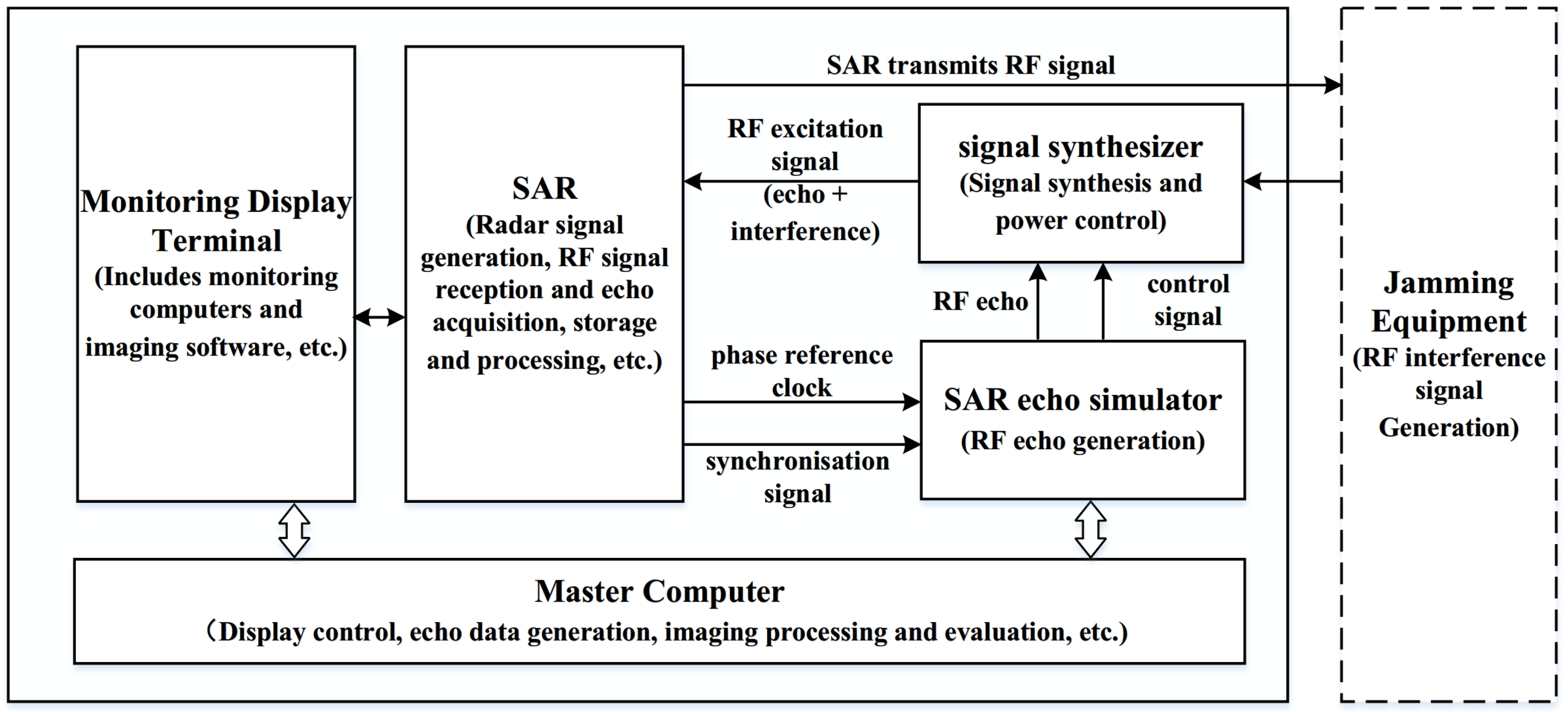
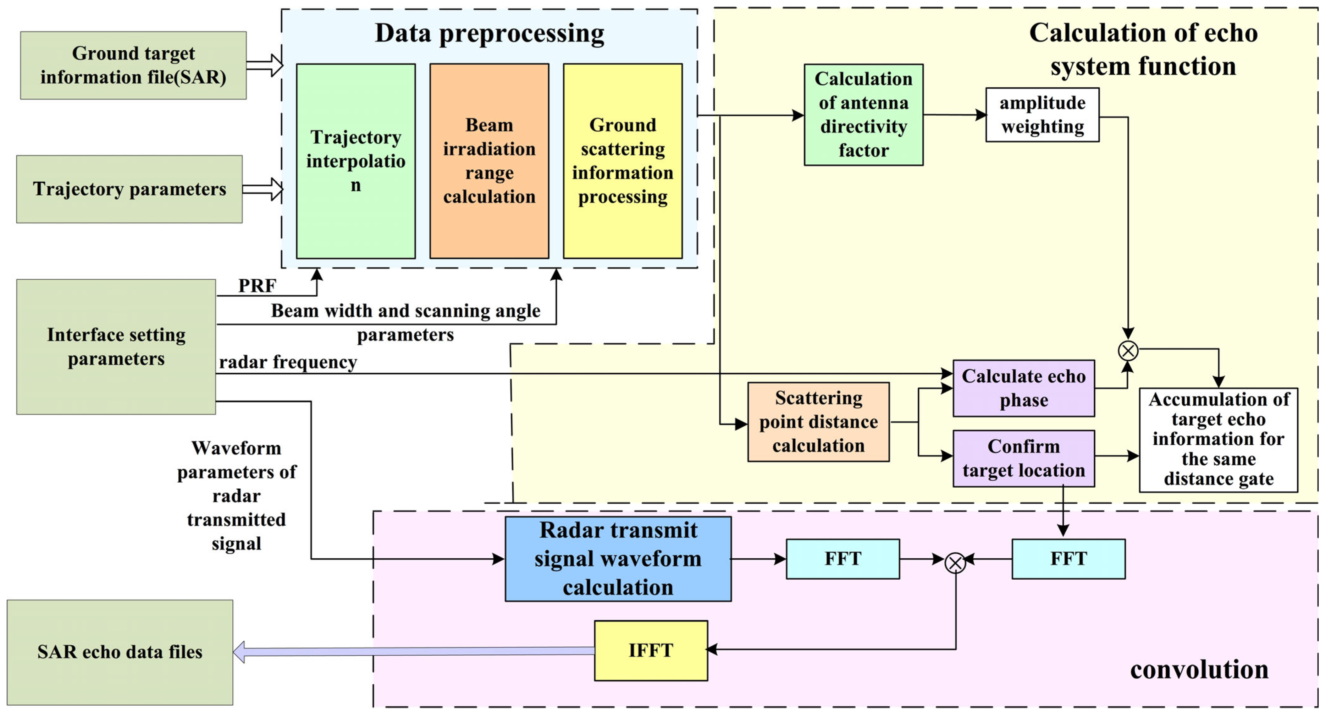
2. Airborne SAR EMI Test System

SAR is a two-dimensional, high-resolution radar system that achieves high resolution in the range direction by transmitting signals with a large time–bandwidth product and employing matched filtering techniques. In the azimuth direction, it utilizes a small aperture antenna mounted on a flying platform. As the platform moves, it emits signals from different locations and then receives the coherent radar echo signals and stores them. Through signal processing methods, it creates the equivalent of a large aperture array antenna to achieve high resolution in the azimuth direction.

However, the dynamic imaging conditions inherent in airborne SAR pose significant replication challenges in static laboratory environments, limiting the practicality of EMI-effect testing in such settings. To overcome this limitation, this study presents a laboratory-based airborne SAR EMI test system. The system emulates airborne SAR imaging processes within static laboratory conditions through integrated operation of signal synthesis modules, a SAR echo simulator, the SAR system hardware, and a master control computer. The system’s integration with vector signal sources enables systematic analysis of EMI-based effects across diverse interference scenarios, validating its capacity for controlled electromagnetic environment simulation. Engineered to replicate airborne SAR’s dynamic imaging characteristics under static constraints, the system effectively executes EMI experiments while maintaining dynamic imaging emulation; its architectural framework is detailed in Figure 1.

Image scene-based SAR echo inversion technology serves as the core methodology that enables the airborne SAR EMI test system to emulate dynamic imaging processes under static conditions. This technique operates through three sequential stages: (1) preprocessing of ground target information and SAR trajectory data, (2) computation of the echo system function, and (3) convolution of the system function with SAR signals. The implementation workflow proceeds as follows: the master computer first employs the range–time domain pulse coherence algorithm to generate digital echo data from input image scenes, which are then converted into RF echo signals via the SAR echo simulator. These signals are subsequently transmitted to the SAR system through RF cabling or antenna radiation to replicate the dynamic imaging processes. The complete implementation architecture is illustrated in Figure 2.

The airborne SAR EMI test system was designed to combine and distribute different types of EMI signals with SAR echo signals through the signal synthesis module. The integrated signal was then transmitted to the SAR system via RF cabling, where it underwent Chirp Scaling (CS) algorithm processing in order to generate the final image output.

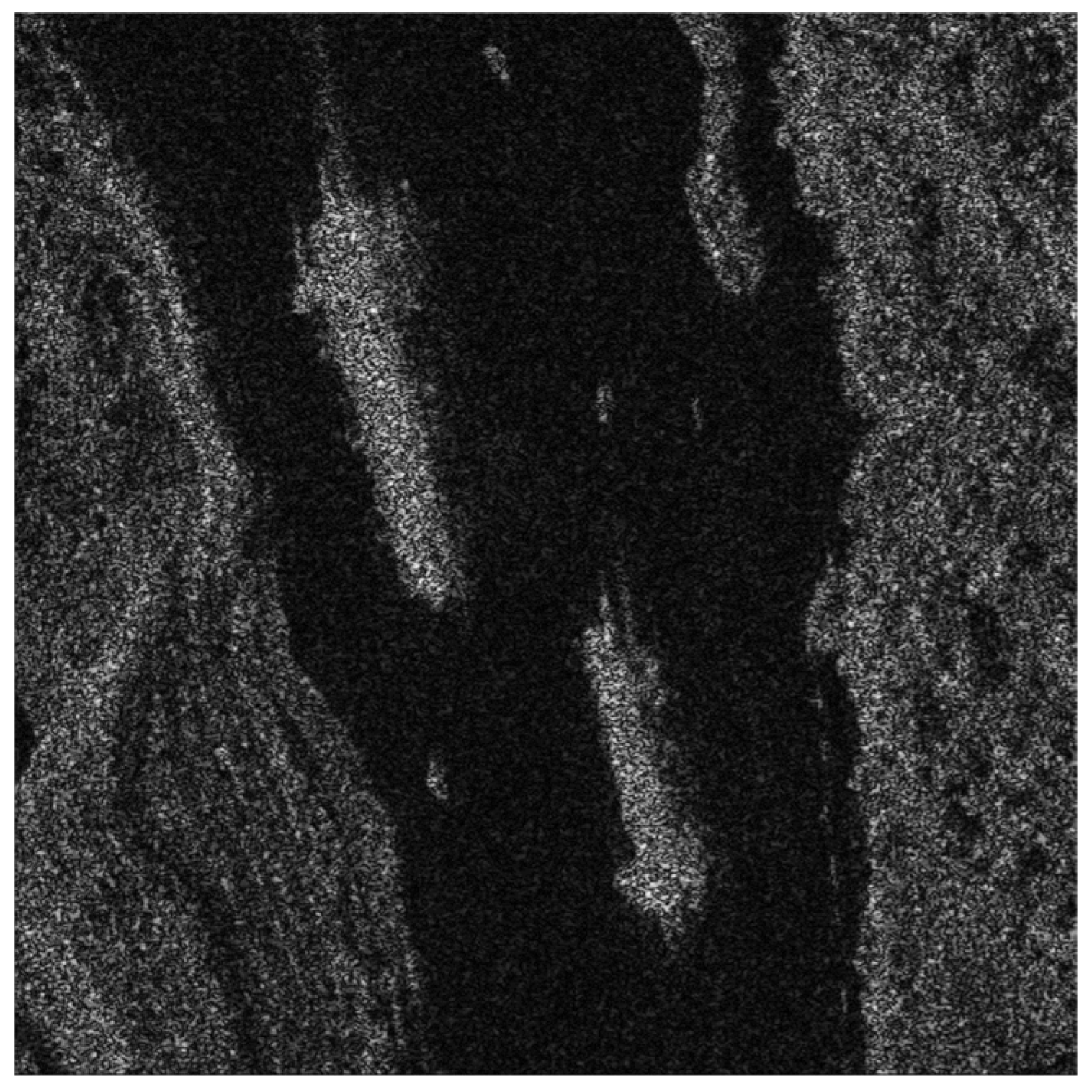
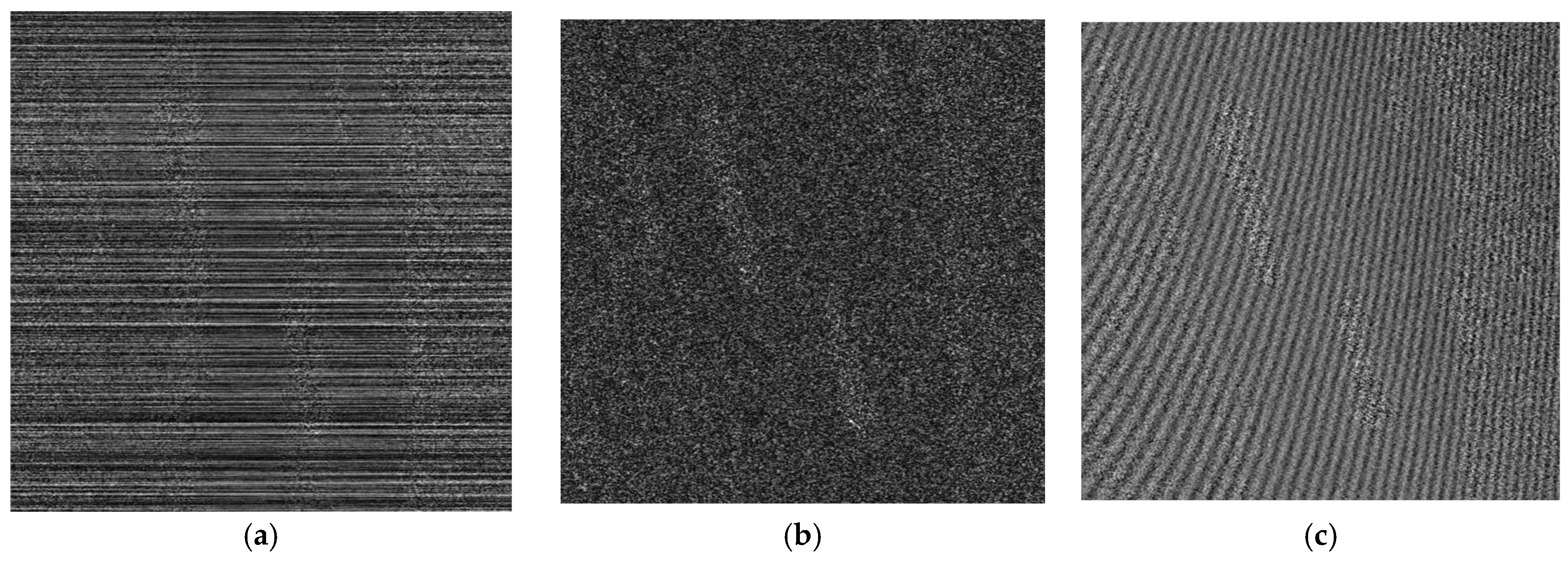
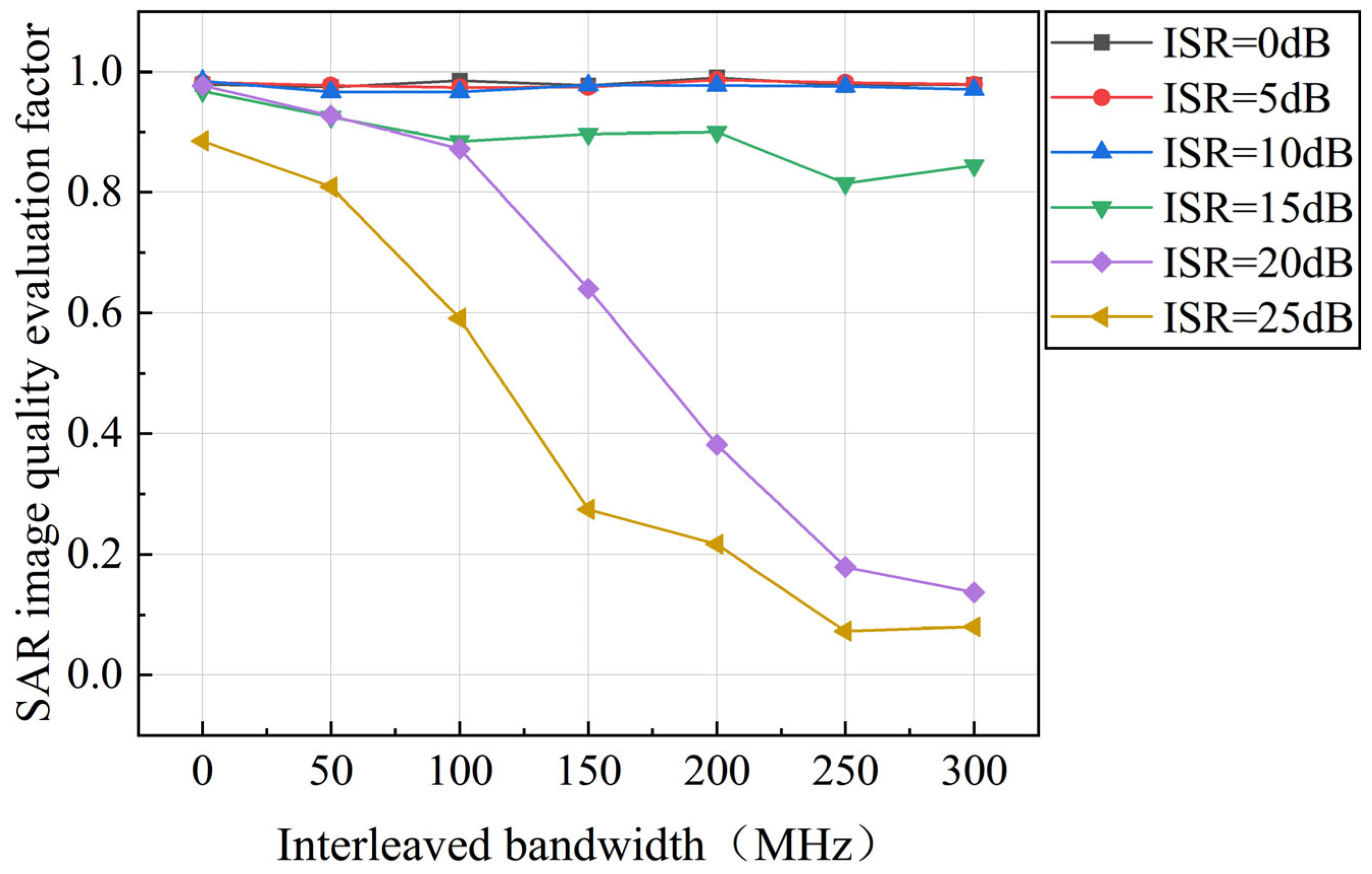
3. Evaluation Method for EMI-Based Effects in SAR Images

To evaluate the impacts of distinct EMI types on airborne SAR imagery, the proposed EMI test system was utilized to assess interference effects across three signal categories: single-frequency continuous wave (SFCW), Gaussian white noise, and linear frequency-modulated continuous wave (LFMCW). Baseline imaging results (without interference) and interference-affected imaging outcomes are presented in Figure 3 and Figure 4, respectively.

The imaging template selected for Figure 3 is image 000243 in the SSDD dataset, which is cropped to a size of 500 × 500 pixels. The image contains, in the background, the coastline’s contour and the two target ships are in the center; the parameters of the test system are set as shown in

Table 1. The parameters for the SAR EMI test system.

Name	Value
SAR imaging mode	strip imaging
Carrier frequency	9 GHz
Signal bandwidth	300 MHz
Pulse width	20 µs
Pulse repetition frequency	1000 Hz
Signal sampling rate	600 MHz
Aircraft platform speed	250 m/s
Range resolution	0.5 m
Azimuth resolution	0.5 m

.

As demonstrated in Figure 3 and Figure 4, the airborne SAR imaging results exhibit distinct interference patterns under different EMI types. White noise manifests as uniformly distributed snowflake-like noise points across the image plane. Single-frequency continuous wave (SFCW) interference generates non-uniform bright line artifacts predominantly oriented in the range direction. Linear frequency-modulated broadband interference signals produce oblique stripe patterns characterized by alternating light–dark intensity variations resembling interference fringes.

To provide objective quantification of SAR image degradation under varied interference conditions, this study adopted three quantitative metrics [34]: Pearson correlation coefficient (PCC), structural similarity (SSIM), and peak signal-to-noise ratio (PSNR).

The Pearson correlation coefficient (PCC) indicates the statistical correlation between two images and can demonstrate the total degree of correlation between the pre-interference image and the post-interference image; this can be can be expressed as

$$PCC={\displaystyle \frac{{\displaystyle \sum _{i=1}^m{\displaystyle \sum _{j=1}^n\left[f\left(x_i,y_j\right)-{\mu }_f\right]\left[g\left(x_i,y_j\right)-{\mu }_g\right]}}}{{\left[{\displaystyle \sum _{i=1}^m{\displaystyle \sum _{j=1}^n{\left[f\left(x_i,y_j\right)-{\mu }_f\right]}^2\ast {\displaystyle \sum _{i=1}^m{\displaystyle \sum _{j=1}^n{\left[g\left(x_i,y_j\right)-{\mu }_g\right]}^2}}}}\right]}^{1/2}}}$$

(1)

where $f\left(x_i,y_j\right)$ is the pre-interference image, $g\left(x_i,y_j\right)$ is the post-interference image, ${\mu }_f$ is the mean value of image $f\left(x_i,y_j\right)$, and ${\mu }_g$ is the mean value of image $g\left(x_i,y_j\right)$. The $m$ and $n$ are the numbers of pixels in the length and width of the images, respectively.

Structure similarity index measure (SSIM) is a measure of the similarity of two images, one which defines structural information as an image attribute, independent of brightness and contrast, from the point of view of image composition; this can be expressed as

$$SSIM={\displaystyle \frac{\left(2{\mu }_f{\mu }_g+C_1\right)\left(2{\sigma }_{fg}+C_2\right)}{\left({\mu }_f^2+{\mu }_g^2+C_1\right)\left({\sigma }_f^2+{\sigma }_g^2+C_2\right)}}$$

(2)

where ${\sigma }_{fg}$ is the covariance between images $f\left(x_i,y_j\right)$ and $g\left(x_i,y_j\right)$, while ${\sigma }_f$ and ${\sigma }_g$ are the standard deviations of images $f\left(x_i,y_j\right)$ and $g\left(x_i,y_j\right)$, respectively. The terms $C_1$ and $C_2$ serve to prevent instability in image regions where local means or standard deviations are close to zero. $C_1={\left(K_{1}L\right)}^2$,$C_2={\left(K_{2}L\right)}^2$ where $L$ is the number of gray levels in the image; for an 8-bit grayscale image, $L$ is taken as 255. The $K_1$ and $K_2$ are small constant values, typically $K_1$ is set to 0.01 and $K_1$ set to 0.03.

Peak signal-to-noise ratio (PSNR) is an objective evaluation index used to evaluate the noise level or image distortion, and is one of the most common and widely used objective evaluation indices for images; it can be expressed as

$$PSNR=20\lg \left\{{\displaystyle \frac{255}{\sqrt{\frac{1}{mn}{\displaystyle \sum _{i=1}^m{\displaystyle \sum _{j=1}^n{\left[f\left(x_i,y_j\right)-g\left(x_i,y_j\right)\right]}^2}}}}}\right\}$$

(3)

Given that the PCC, SSIM, and PSNR have different dimensions, to balance the dimensions of each parameter and facilitate subsequent processing by predictive models, normalization was applied to all three. The normalization formula can be expressed as

$$X_{\mathrm{norm}}={\displaystyle \frac{X-X_{\min }}{X_{\max }-X_{\min }}}$$

(4)

where $X_{\mathrm{norm}}$ is the normalized sample value, $X$ is the original sample value before normalization, $X_{\min }$ is the minimum value of the sample, and $X_{\max }$ is the maximum value of the sample.

To integrate the different evaluation weights of the PCC, SSIM, and PSNR relative to the images, this study introduces a novel SAR image-quality evaluation factor, which is denoted by $Q_f$. The calculation method for $Q_f$ can be expressed as

$$Q_f=w_1\times PCC+w_2\times SSIM+w_3\times PSNR$$

(5)

where $w_1$, $w_2$, and $w_3$ are the weights of the PCC, SSIM, and PSNR indicators, respectively.

It should be clarified that this study adopts an equal-weight strategy with minimal subjective intervention to prevent distorted evaluation outcomes caused by single-indicator bias, ensuring balanced sensitivity of quality assessment metrics to multiple interference types in SAR image evaluation. Specifically, the weights are set as $w_1=w_2=w_3=1/3$, ensuring that the $Q_f$ value falls within the range [0,1]. This design allows the omission of data normalization steps during the subsequent model training described in later sections.

Since PCC, SSIM and PSNR are negatively correlated with the degree of image interference, the higher the degree of image interference, the lower the image evaluation factor $Q_f$.

Utilizing the SAR image-quality evaluation factor $Q_f$, this study assessed the results of airborne SAR EMI-effect experiments with different types of interference signals and various interference signal parameters and then visualized the obtained results.

To study the influence of single-frequency continuous wave signal interference on SAR images, experiments were conducted to obtain single-frequency continuous wave interference with respect to SAR images, under different frequencies and interference-to-signal ratios (ISRs). The ISR can be expressed as

$$ISR=10\log \left({\displaystyle \frac{P_j}{P_r}}\right)$$

(6)

where $P_j$ is the interference signal power and $P_r$ is the echo signal power.

The SAR image interference evaluation factor was calculated for all images, and the variation in the SAR image interference evaluation factor with the frequency of the single-frequency continuous wave signal is shown in Figure 5.

Figure 5 shows that when the ISR does not exceed 15 dB, the closer the interference frequency is to 9 GHz, the more obvious the SAR image interference effect, and the corresponding SAR image interference evaluation factor value is lower. When the ISR exceeds 20 dB, the interference effect is essentially similar within the frequency range of 8.5 GHz to 9.5 GHz and has little correlation with frequency. When the interference signal falls outside the range of 8.5 GHz to 9.5 GHz, the interference signal cannot have a significant impact on the imaging results due to the frequency selection effect associated with the receiver’s multi-stage filters.

For Gaussian white noise interference, the signal bandwidth was fixed to 100 MHz, and the signal frequency and the ISR conditions were changed. The results obtained for the interference experiments under different signal frequencies and ISR conditions are shown in Figure 6.

As illustrated in Figure 6, when the ISR is higher than 15 dB but lower than 30 dB, the closer the Gaussian white noise signal frequency is to 9 GHz, the lower the SAR image interference assessment factor, which shows the more noticeable SAR image interference effect. When the ISR is higher than or equal to 30 dB and the interference frequency is within the radar working bandwidth (8.5 GHz–9.5 GHz), the correlation between the SAR image interference evaluation factor and the interference signal frequency gradually decreases as the ISR increases. This indicates that when the ISR reaches a certain level, the SAR image interference effect becomes saturated and the correlation with noise interference signal frequency ceases to obtain.

To investigate the effect of the overlapping frequency band size in the bandwidth of the Gaussian white noise signal and the working bandwidth of the radar on the interference effect, the signal bandwidth of the Gaussian white noise was fixed at 1000 MHz, and its center frequency was changed from 7.9 GHz to 9 GHz with a step size of 100 MHz, thereby changing the size of the overlapping frequency band from the shared bandwidth of the white noise signal and the working bandwidth of the radar. Figure 7 depicts the variation law of the SAR image interference assessment factor with overlapping bandwidth under the same ISR settings.

As shown in Figure 7, when the ISR is lower than 20 dB, the interference energy introduced into the SAR system by different interleaved bandwidths is at a low level, and the effect of the different interleaved bandwidths is closer to SAR interference. When the ISR is higher than 20 dB or lower than 32 dB, under the condition of the same ISR, the SAR image-quality evaluation factor decreases with the increase in the interfering overlapping bandwidth when the overlapping bandwidth is lower than or equal to 600 MHz, and the SAR image-quality evaluation factor remains close to the same level when the overlapping bandwidth is higher than 600 MHz. When the ISR reaches 35 dB, the SAR image-quality evaluation factor does not decrease with the increase in the overlapping bandwidth, as long as the overlapping bandwidth reaches a value higher than than 300 MHz.

To research the influence of interference frequency deviation on the interference effect, experiments on the interference effects of LFMCW with different center frequencies were carried out. The frequency modulation (FM) bandwidth was fixed to 300 MHz, the FM rate was fixed to 15 Hz/µs, and the FM period was fixed to 20 µs. The experiments obtained the interference variation law of the SAR image given the interference of LFMCW signals at different frequencies; the results are shown in Figure 8.

Figure 8 shows that there is no significant correlation between the SAR image interference evaluation factor and the frequency of the interference signal, as long as the bandwidth of the interference signal is completely within the radar’s working bandwidth and the ISR is fixed. The primary reason for this is that, while the center frequency of the LFMCW signal changes, it still has a particular signal bandwidth, allowing most of the energy to enter the SAR system, and generating interference effects on the SAR image.

Relevant interference experiments were carried out to explore the influence of the size of the overlapping frequency band, located between the bandwidth of LFMCW signals and the radar working bandwidth, on the interference effect. In the experiments, the FM bandwidth was fixed at 300 MHz and the FM rate was fixed at 15 Hz/µs, and the overlapping band between the LFMCW signal bandwidth and the radar working bandwidth was changed by changing the center frequency of the LFMCW signal. Figure 9 depicts the experimental results for LFMCW signal interference over various overlapping frequency bands.

Figure 9 shows that when the ISR is lower than or equal to 10 dB, the SAR image interference evaluation factor essentially remains constant with the fluctuation of overlapping frequency bands, and the image has no interference effect. When ISR is 15 dB, the SAR image interference evaluation factor decreases with the increase in the overlapping frequency band, but the decrease is small, and the SAR image interference evaluation factor basically stays above 0.8, indicating that the interference effect is not obvious. When the ISR is higher than or equal to 20 dB, the SAR image interference evaluation factor decreases with the increase in the overlapping frequency band, and the SAR image interference effect is more obvious with the increase in the overlapping frequency band under the same ISR condition.

Based on the above analysis, the following laws can be determined:

(1) The interference results and nominal behavior exhibited by airborne SAR under different types of interference signals are different.

(2) The interference effect caused by the interference signal is more visible the closer the interference signal frequency is to the radar center frequency, or the smaller the frequency deviation between the interference signal and the radar center frequency. Furthermore, the quality of images is unaffected by interference signals with frequencies outside the radar’s working frequency range.

(3) The relationship between the SAR image-quality evaluation factor and the interference signal frequency is basically symmetrical around the center of the radar frequency.

(4) Under the condition of fixed frequency offset and ISR, the larger the overlap in bandwidth between the interference signal frequency band and the radar working frequency band, the more obvious the interference effect, and the lower the SAR image-quality evaluation factor.

4. NRBO–XGBoost Prediction Algorithm

With improvements in computer computing power, big data analysis technology has become widely used in various fields. Machine learning, as one of its branches, has been widely used in computer vision, natural language processing, and the modelling and prediction of various engineering problems due to its ability to automatically identify data patterns and return a good prediction effect.

Airborne SAR systems often encounter complex electromagnetic environments during reconnaissance missions. Modern military aircraft typically incorporate spectrum sensing modules capable of detecting external electromagnetic signals. When these modules detect unknown signals, rapid assessment of their potential to degrade SAR image quality—and consequently affect target detection and situational awareness—is critical. To enhance airborne SAR systems’ ability to evaluate the threat levels associated with unknown electromagnetic signals, a prediction model based on the NRBO–XGBoost algorithm is proposed. This methodology innovatively employs the NRBO algorithm to identify optimal hyperparameters in the XGBoost model, enabling accurate prediction of multidimensional, high-dimensional SAR EMI test data. The developed model provides a quantitative basis for assessing threats to SAR detection capabilities, supporting aircraft avoidance strategies and intelligent anti-jamming operations.

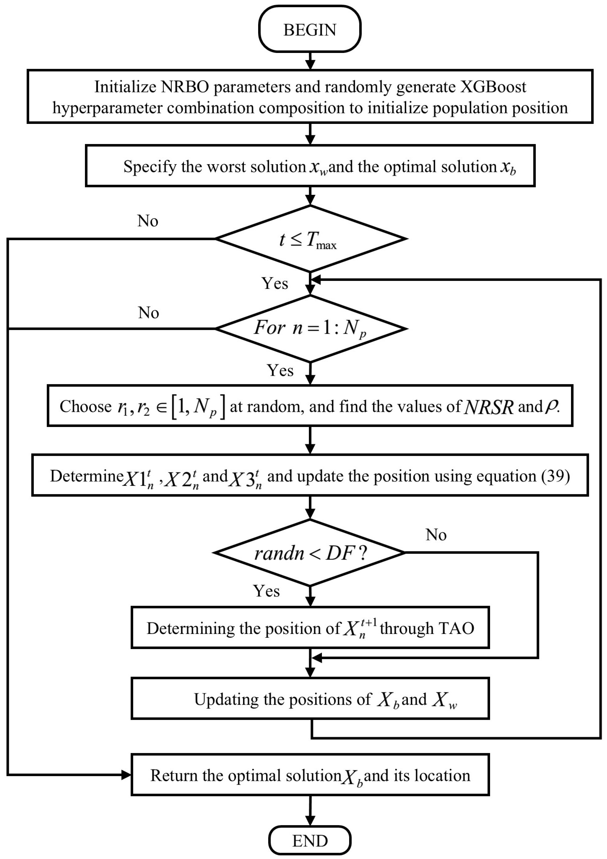
4.1. Optimization of Hyperparameters by NRBO Algorithm

The NRBO algorithm is a novel intelligent optimization algorithm proposed by Sowmya et al. [32] in 2024. Inspired by the Newton–Raphson method, the author uses the Newton–Raphson search rule (NRSR) and trap avoidance operator (TAO) to explore the entire search process and further explores the best results using several sets of matrices. The following introduces the optimization principle of the NRBO algorithm based on three aspects: population initialization, NRSR, and TAO.

4.1.1. Population Initialization

Assuming optimization is performed for an unconstrained single-objective optimization problem, the optimization objective can be expressed as

$$\begin{array}{l}M\mathrm{inimize}:f\left(x_1,x_2,\dots x_n\right)\\ lb\le x_j\le ub,j=1,2,\dots dim\end{array}$$

(7)

where $f\left(x\right)$ is the minimum fitness function, $x_j$ represents the decision vector, $dim$ is the dimension of the problem, and $lb$ and $ub$ are the lower and upper limits of the parameters to be optimized, respectively.

NRBO searches for the optimal solution by generating random populations in the boundary region of the candidate solution, based on $N_p$ populations, and each population is composed of $dim$ decision variables. Therefore, the expression for generating the random population is

$$x_j^n=lb+rand\times \left(ub-lb\right)$$

(8)

where $x_j^n$ is the $j$-th dimensional position of the $n$-th population and $rand$ is a random number in the range of $\left(0,1\right)$. The population matrix expression containing all dimensional populations can be expressed as

$$X_n=\left[\begin{array}{cccc}{x}_1^1& x_2^1& \dots & x_{dim}^1\\ x_1^2& x_2^2& \dots & x_{dim}^2\\ ⋮& ⋮& \ddots & ⋮\\ x_1^{N_p}& x_2^{N_p}& \dots & x_{dim}^{N_p}\end{array}\right]$$

(9)

4.1.2. Newton–Raphson Search Rule (NRSR)

The NRSR uses the idea of the Newton reason method (NRM) to promote the search trend and speed up the convergence speed of the algorithm. Because the objective functions of many optimization problems are not differentiable, the NRM method used in mathematics cannot directly replace the explicit formula of the function. Therefore, NRSR starts from a hypothetical initial solution and advances in a certain direction to the next position to simulate the search process associated with NRM. The position update formula can be expressed as

$$x_{n+1}=x_n-{\displaystyle \frac{\left[f\left(x_n+\Delta x\right)-f\left(x_n-\Delta x\right)\right]\times \Delta x}{2\times \left[f\left(x_n+\Delta x\right)+f\left(x_n-\Delta x\right)-2\times f\left(x_n\right)\right]}}$$

(10)

Considering the population-based search method, the modified NRSR formula can be expressed as

$$NRSR=randn\times {\displaystyle \frac{\left(X_w-X_b\right)\times \Delta x}{2\times \left(X_w+X_b-2\times x_n\right)}}$$

(11)

where $randn$ is a normal distribution random number with mean value of 0 and variance of 1, $X_w$ is the worst position, and $X_b$ is the best position.

To balance the exploration and development ability of the algorithm and avoid falling into the optimal solution prematurely, the adaptive coefficient $\delta$ is introduced to enhance the algorithm. The expression of $\delta$ is

$$\delta ={\left[1-\left({\displaystyle \frac{2\times t}{T_{\max }}}\right)\right]}^5$$

(12)

where $t$ is the current iteration number and $T_{\max }$ is the maximum iteration number.

When combined with adaptive parameter $\delta$, NRSR avoids falling into local optimization by adding random actions in the optimization process. The expression $\Delta x$ in Formula (11) is

$$\Delta x=rand\left(1,dim\right)\times \left|X_b-X_n^t\right|$$

(13)

where $X_b$ is the currently obtained optimal solution, and $rand\left(1,dim\right)$ is a random number with a $dim$-dimensional decision variable.

The NRSR is then introduced, and Formula (10) is modified:

$$x_{n+1}=x_n-NRSR$$

(14)

And the parameter $\rho$ is introduced to improve the development process of the proposed NRSR, which is used to guide the population to the right direction, and its expression is

$$\rho =a\times \left(X_b-X_n^t\right)+b\times \left(X_{r1}^t-X_{r2}^t\right)$$

(15)

where $a$ and $b$ are random numbers in the range of $\left(0,1\right)$, and $r_1$ and $r_2$ are different integers randomly selected from the population.

The current position of the vector is updated by Equation (16).

$$X{1}_n^t=x_n^t-\left[randn\times {\displaystyle \frac{\left(X_w-X_b\right)\times \Delta x}{2\times \left(X_w+X_b-2\times X_n\right)}}\right]+\left[a\times \left(X_b-X_n^t\right)+b\times \left(X_{r1}^t-X_{r2}^t\right)\right]$$

(16)

where $X{1}_n^t$ is the new vector position obtained by updating $x_n^t$. The NRSR is further improved through NRM, and Formula (11) is updated as follows:

$$NRSR=randn\times {\displaystyle \frac{\left(y_w-y_b\right)\times \Delta x}{2\times \left(y_w+y_b-2\times x_n\right)}}$$

(17)

$$y_w=c\times \left[Mean\left(Z_{n+1}+x_n\right)+c\times \Delta x\right]$$

(18)

$$y_b=c\times \left[Mean\left(Z_{n+1}+x_n\right)-c\times \Delta x\right]$$

(19)

$$Z_{n+1}=x_n-randn\times {\displaystyle \frac{\left(X_w-X_b\right)\times \Delta x}{2\times \left(X_w+X_b-2\times x_n\right)}}$$

(20)

where $y_w$ and $y_b$ are the positions of two vectors generated using $Z_{n+1}$ and $x_n$, and $c$ represents a random number in the range of $\left(0,1\right)$.

Using the improved NRSR update Formula (16), the updated formula is

$$X{1}_n^t=x_n^t-\left[randn\times {\displaystyle \frac{\left(y_w-y_b\right)\times \Delta x}{2\times \left(y_w-y_b-2\times x_n\right)}}\right]+\left[a\times \left(X_b-X_n^t\right)+b\times \left(X_{r1}^t-X_{r2}^t\right)\right]$$

(21)

Using the optimal vector $X_b$ to replace the current vector $x_n^t$ in Equation (21), a new position vector is constructed, as

$$X{2}_n^t=X_b-\left[randn\times {\displaystyle \frac{\left(y_w-y_b\right)\times \Delta x}{2\times \left(y_w-y_b-2\times x_n\right)}}\right]+\left[a\times \left(X_b-X_n^t\right)+b\times \left(X_{r1}^t-X_{r2}^t\right)\right]$$

(22)

The development phase is the focus of the search direction strategy. In local search, the search method proposed in Equation (22) is virtuous, but it has limitations when it comes to global search, whereas the search strategy presented by Equation (21) is virtuous for global search but has limitations when it comes to local search. Therefore, the NRBO uses both Equations (21) and (22) to improve the diversification and intensification phases.

The formula for updating the final position vector is

$$x_n^{t+1}=d\times \left[d\times X{1}_n^t+\left(1-d\right)\times X{2}_n^t\right]+\left(1-d\right)\times X{3}_n^t$$

(23)

$$X{3}_n^t=X_n^t-\delta \times \left(X{2}_n^t-X{1}_n^t\right)$$

(24)

4.1.3. Trap Avoidance Operation (TAO)

TAO is introduced to improve the efficiency of the NRBO algorithm in dealing with practical optimization problems. TAO can greatly change the position of $x_n^{t+1}$ and generate an enhanced solution $X_{TAO}^t$ by combining the optimal positions $X_b$ and $X_n^t$. When the value of $rand$ is less than the NRBO performance determining factor $DF$, $X_{TAO}^t$ is updated to

$$\left\{\begin{array}{c}\begin{array}{c}{X}_{TAO}^t=X_n^{t+1}+{\theta }_1\times \left({\mu }_1\times x_b-{\mu }_2\times X_n^t\right)+{\theta }_2\times \delta \\ \times \left[{\mu }_1\times Mean\left(X^t\right)-{\mu }_2\times X_n^t\right],{\mu }_1<0.5\end{array}\\ \begin{array}{c}{X}_{TAO}^t=x_b+{\theta }_1\times \left({\mu }_1\times x_b-{\mu }_2\times X_n^t\right)+{\theta }_2\times \delta \\ \times \left[{\mu }_1\times Mean\left(X^t\right)-{\mu }_2\times X_n^t\right],{\mu }_1\ge 0.5\end{array}\end{array}\right.$$

(25)

$$X_n^{t+1}=X_{TAO}^t$$

(26)

where ${\theta }_1$ and ${\theta }_2$ are uniform random numbers in the ranges of (−1, 1) and (−0.5, 0.5), respectively. ${\mu }_1$ and ${\mu }_2$ are random numbers, which are generated by Formulas (27) and (28), respectively.

$${\mu }_1=\left\{\begin{array}{c}3\times rand,if\Delta <0.5\\ 1, Otherwise\end{array}\right.$$

(27)

$${\mu }_2=\left\{\begin{array}{c}rand,if \Delta <0.5\\ 1, Otherwise\end{array}\right.$$

(28)

where $\Delta$ is a random number in the range of (0, 1).

4.1.4. Mathematical Intuition of the NRBO Algorithm

The core innovation of the NRBO algorithm is to combine the second-order convergence property of Newton’s method with population intelligence optimization. The traditional Newton’s method quickly approximates the extreme point by the iterative formula $x_{n+1}=x_n-{\displaystyle \frac{f\left(x_n\right)}{f^{\prime }\left(x_n\right)}}$, but its dependence on the derivability of the objective function limits its application in complex optimization problems. The NRBO overcomes this limitation through the following mathematical mechanisms:

(1) Gradient approximation: In non-directable scenarios, the gradient direction is modeled using the population difference $X_w-X_b$ (Equation (11)), and the exploratory capability is introduced through the random vector $rand\left(1,dim\right)$ (Equation (13)).

(2) Second-order convergence properties: The adaptive coefficient $\delta$ (Equation (12)) dynamically balances global exploration (large-scale search) and local exploitation (fine optimization), and its exponential decay properties are consistent with the step-size reduction law of Newton’s method.

(3) Trap Avoidance Operator (TAO): Generating the perturbation term $X_{TAO}^t$ through Equations (25)–(28) is mathematically equivalent to introducing a random regular term in the loss function to avoid falling into the local minima.

To systematically evaluate the distinctiveness and superior performance of the NRBO against other optimization algorithms, a comparative analysis of algorithmic performance is presented in

Table 2. Summary of the performance comparisons between the NRBO algorithm and other optimization algorithms.

Evaluation Criterion	NRBO	Gradient-Free Algorithms (e.g., PSO [35], GA [36], and DE [37])	Other Swarm Intelligence Algorithms (e.g., GWO [38], HHO [39])
Convergence Speed	Leverages gradient directions for accelerated convergence; Reduced iteration counts by 30–50% in CEC2017 benchmarks.	Rely on stochastic search mechanisms, resulting in slower convergence rates.	Moderate convergence speed with susceptibility to local oscillations.
Global Exploration	TAO mechanism enhances population diversity; Balance index > 90% across 23 benchmark functions.	Prone to premature convergence, diversity degradation in high-dimensional spaces.	Limited exploration capabilities, parameter-sensitive performance.
Local Exploitation	NRSR strategy enables precise extremum approximation; Standard deviation < 1 × 10−10 in CEC2022 composite functions.	Lacks gradient guidance, inefficient local development.	Neighborhood-based search with precision constraints.
High-Dimensional Adaptability	Maintains stability in 1000D problems, outperforms GBO [40]/RKO [41].	Suffers from “curse of dimensionality”, performance collapse.	Certain algorithms (e.g., EO [42]) exhibit suboptimal scalability.
Engineering Applicability	Achieved optimal solutions in 12/12 CEC2020 engineering optimization problems.	Feasibility constraint violations in complex scenarios.	Requires extensive parameter tuning; limited robustness.

. The experimental data for the NRBO have been directly extracted from the original research article [34], ensuring methodological consistency in benchmarking.

As demonstrated in Table 2, the NRBO exhibits statistically significant superiority across the convergence speed, global search capability, and high dimensional adaptability critical attributes that distinguish it from conventional gradient-free algorithms and other swarm intelligence approaches.

These algorithmic advantages become particularly valuable when addressing complex real-world optimization challenges. One representative application domain lies in hyperparameter tuning for machine learning models, an area in which traditional manual search methods face inherent limitations in balancing exploration–exploitation trade-offs. This context provides an ideal testbed to validate the NRBO’s practical effectiveness through its integration with XGBoost—a widely adopted gradient-boosting framework known for its powerful predictive capabilities but constrained by hyperparameter sensitivity. The hyperparameter space of the XGBoost algorithm is shown in

Table 3. The hyperparameter space of the XGBoost model.

Name	Mean
Learning rate	Control the scaling of each tree’s weights
Max depth	Limit the maximum depth of the tree to prevent overfitting
Subsample	Proportion of samples used to train each tree
Column sample by tree	Proportion of feature columns used to train each tree
Min child weight	Sum of weights controlling further division of leaf nodes
Gamma	Minimum gain threshold to control further cutting of leaf nodes
Reg lambda	L2 regularization factor for controlling model complexity
Reg alpha	L1 regularization factor for controlling model complexity
Scale pos weight	Weighting adjustment factors for dealing with category imbalances

.

Table 3 shows that XGBoost has a vast hyperparameter search space during training, involving multidimensional combinations of parameters such as learning rate, max depth, and regularization terms. Traditional hyperparameter selection relies heavily on empirical heuristics and domain expertise, making manual exploration inefficient and prone to suboptimal solutions. The integration of NRBO introduces an intelligent search mechanism that systematically navigates this complex parameter landscape. By leveraging the NRBO’s enhanced exploration–exploitation balance, the hybrid approach not only improves XGBoost’s prediction accuracy and generalization performance but also effectively mitigates overfitting/underfitting risks. This dual optimization of model fitting capability and structural complexity is further visualized through the iterative search process detailed in Figure 10.

4.2. Indicators for Model Evaluation

After the training of the machine learning model is completed, some statistical metrics can be used to evaluate the prediction performance of the model, including root mean squared error (RMSE), mean absolute error (MAE), Euclidean distance (ED), coefficient of determination (R²), etc.

The RMSE determines the root of the mean squared difference between the predicted values and the true values and indicates the average degree of deviation between the predicted values and the true values, which can be expressed as

$$RMSE=\sqrt{{\displaystyle \frac{1}{m}}{\displaystyle \sum _{i=1}^m{\left(y_i-{\widehat{y}}_i\right)}^2}}$$

(29)

where $m$ is the number of samples, $y_i$ is the true value, and ${\widehat{y}}_i$ is the predicted value.

The MAE represents the average value of the absolute error between the predicted value and the observed value, which can be expressed as

$$MAE={\displaystyle \frac{1}{m}}{\displaystyle \sum _i^m\left|y_i-{\widehat{y}}_i\right|}$$

(30)

The ED measures the straight-line distance between two points in Euclidean space, extends it to high-dimensional space, and can represent the similarity between two vectors or two-dimensional arrays; this can be expressed as

$$ED=\sqrt{{\displaystyle \sum _{i=1}^m{\left(y_i-{\widehat{y}}_i\right)}^2}}$$

(31)

The R² is an important statistical index in regression analysis, which describes the degree of interpretation of the prediction model relative to data variation, that is, the prediction accuracy of the prediction model. The determination coefficient ranges from 0 to 1. The closer the value is to 1, the better the prediction effect of the model is. It can be expressed as

$$R^2=1-{\displaystyle \frac{{\displaystyle \sum _{i=1}^m{\left(y_i-{\widehat{y}}_i\right)}^2}}{{\displaystyle \sum _{i=1}^m{\left(y_i-y_{ave}\right)}^2}}}$$

(32)

where $y_{ave}$ is the average of the true values.

5. Model Training Results and Analysis

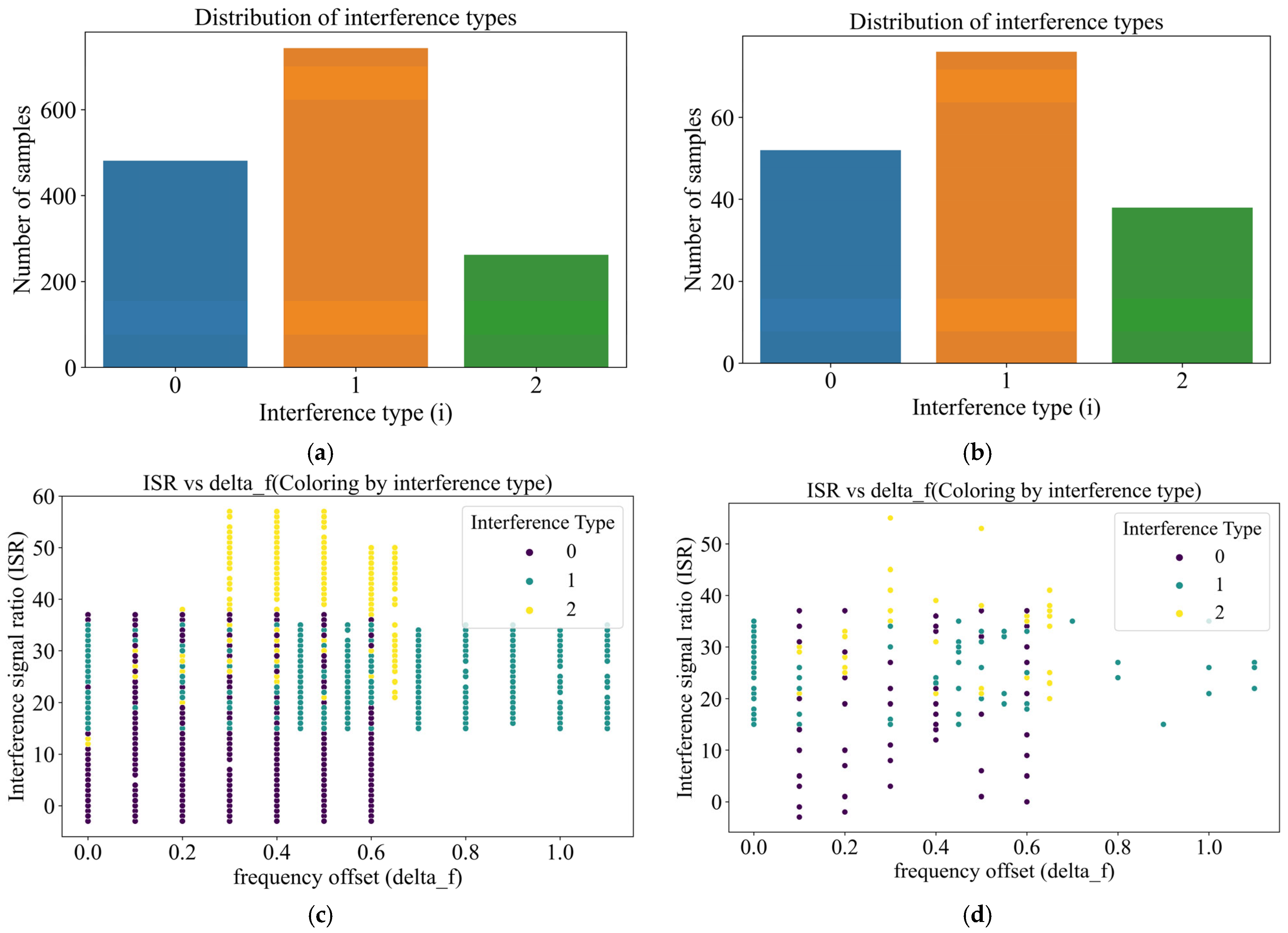
5.1. Feature Selection and Data Sets

According to the EMI-effect law for the SAR images mentioned above, the interference signal parameters that affect the degradation effect of the SAR image include signal type, frequency offset between the interference signal and the center frequency of radar, ISR, and the overlap bandwidth between the interference signal and the radar working frequency band.

Therefore, the above four signal parameters can be used as input variables, and the quality evaluation factor for the SAR images can be used as an output variable to construct a SAR electromagnetic environment effect prediction model. The model can be expressed as

$${\widehat{Q}}_f=F\left(i,\Delta f,\Delta B,ISR\right)$$

(33)

where ${\widehat{Q}}_f$ is the model prediction value, $F\left(\cdot \right)$ is the prediction model, $i$ is the interference signal type number, the single-frequency continuous wave is 0, the white noise is 1, the LFMCW signal is 2, $\Delta f$ is the frequency difference between the frequency of the interference signal and the center frequency of the radar, $\Delta B$ is the size of the overlapping band between the interference signal and the radar working frequency band, and ISR is the power ratio of the interference signal and the echo signal.

This study acquired airborne SAR images under varying interference types and parameters using an onboard SAR EMI testing system and calculated the corresponding SAR image-quality assessment metrics. A total of 1652 experimental datasets were collected through airborne SAR EMI experiments and randomly divided into training sets and test sets prior to model training, at a ratio of 9:1.

To ensure the training set adequately represents the complex distribution characteristics of the test space and to identify potential data shift risks, this research analyzed the data distributions of the training and test sets; the results are shown in Figure 11. According to Figure 11, the training set and test set exhibit statistically consistent patterns in key feature dimensions such as interference type, interference frequency offset, and ISR, validating the rationality of our data division strategy.

To fully utilize this well-structured data configuration, enhance model evaluation robustness, and reduce overfitting risks, this study adopts a 5-fold cross-validation strategy for model training. Specifically, the training set is equally divided into five subsets, with four subsets used for model training and the remaining subset used for performance validation during each iteration. The model weights achieving the minimum loss on the validation set are selected as the optimal solution, and are then applied to the inference phase of the test set.

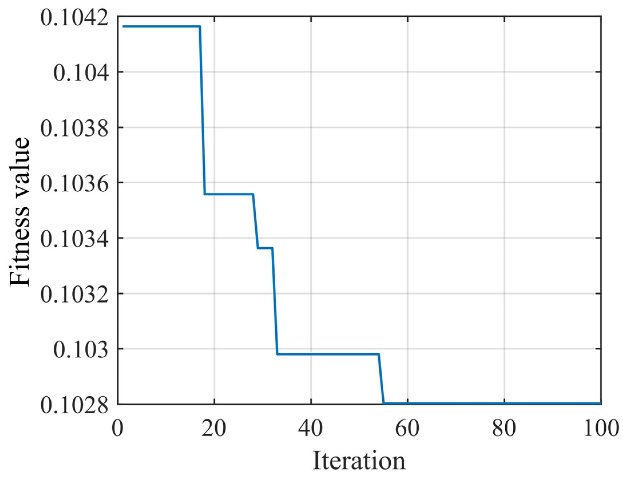
5.2. Model Training Results

Training was conducted using the training set against the XGBoost algorithm, and the hyperparameter space of XGBoost was optimized using the NRBO algorithm. Then, the model performance was validated through the validation set and the prediction error of the model was analyzed. The optimization process for the NRBO algorithm is shown in Figure 12, the comparison between predicted results and true values is shown in Figure 13, and the fitting chart is shown in Figure 14.

According to Figure 12, the NRBO algorithm converges when the number of iterations in the optimization process reaches about 60 and jumps out of the local optimum four times, which indicates good optimization accuracy and convergence speed. According to Figure 13 and Figure 14, the predicted value obtained by the prediction model fits well with the true value regression.

The error between the model’s predicted values and the true values of the validation set is shown in Figure 15, and the histogram of the statistical distribution of the error is shown in Figure 16.

According to Figure 15 and Figure 16, the error between the predicted value of the model and the true value of the validation set is mainly concentrated in [−0.1, 0.1], the number of samples associated with an error of close to 0 is higher than 240, and the error value of individual points reaches about 0.4, accounting for about 3% of the overall data. Therefore, after the optimization of the NRBO algorithm, the XGBoost prediction model has high prediction accuracy and can realize the accurate prediction of airborne SAR environmental electromagnetic effects.

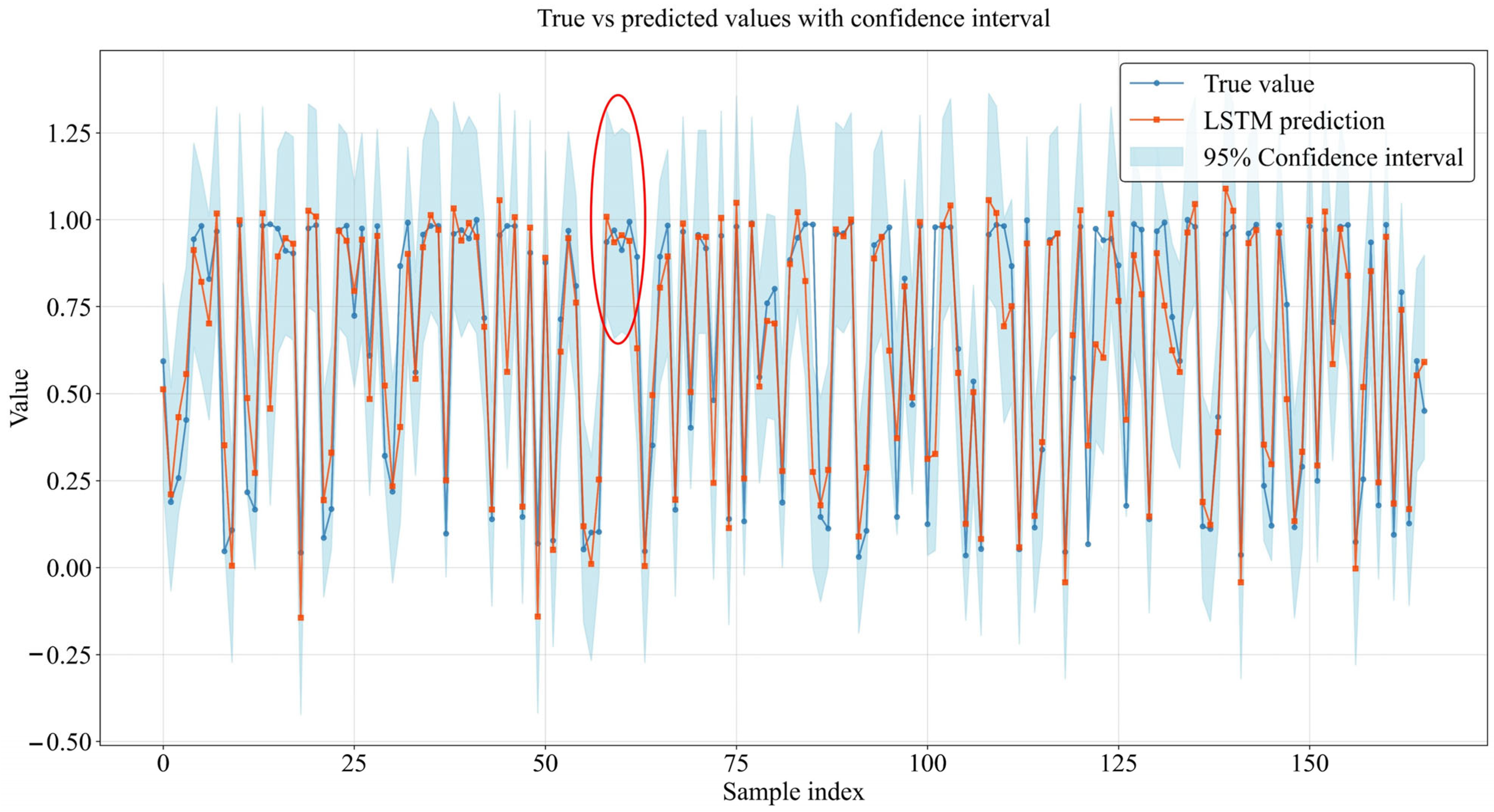
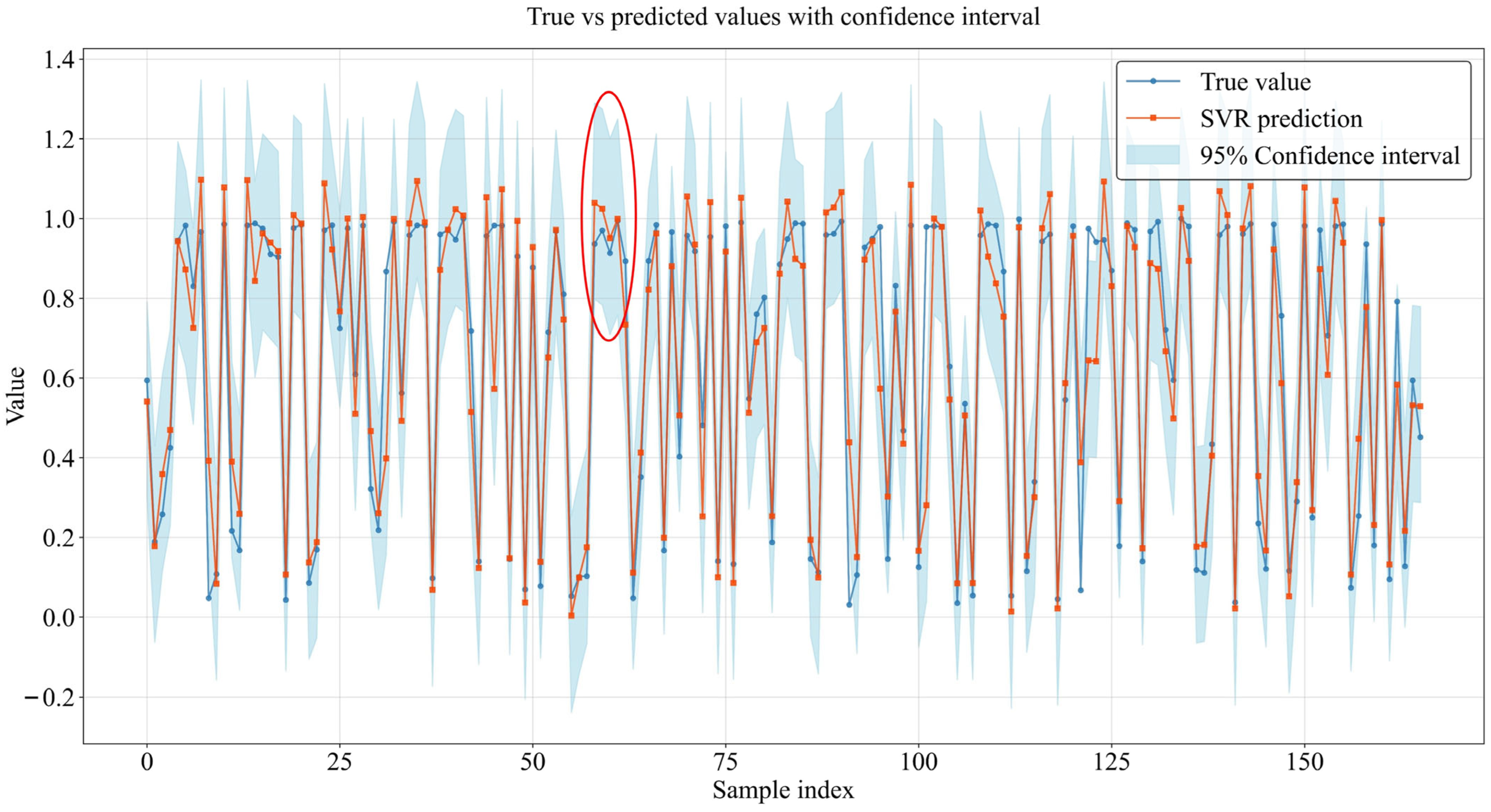
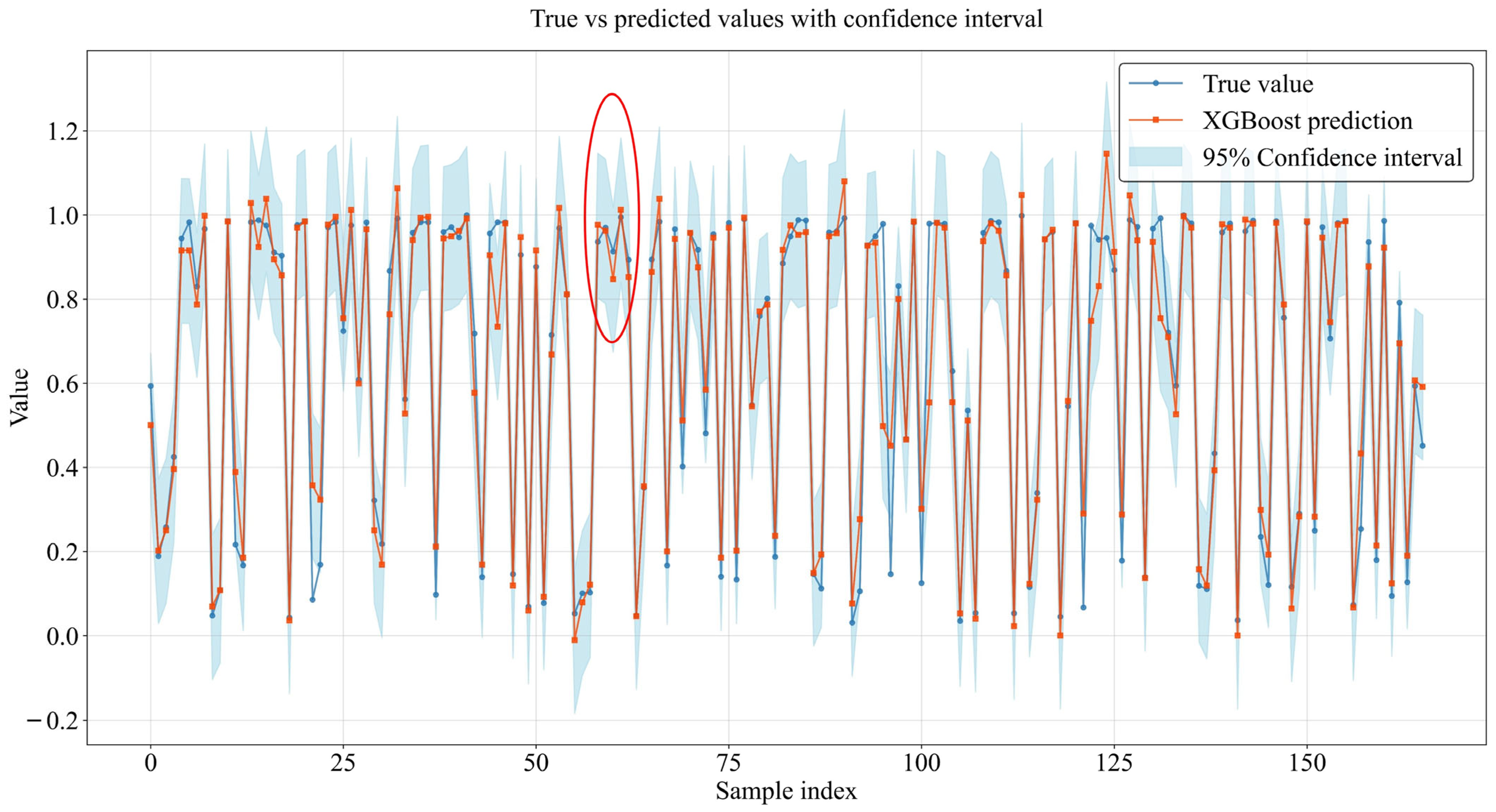
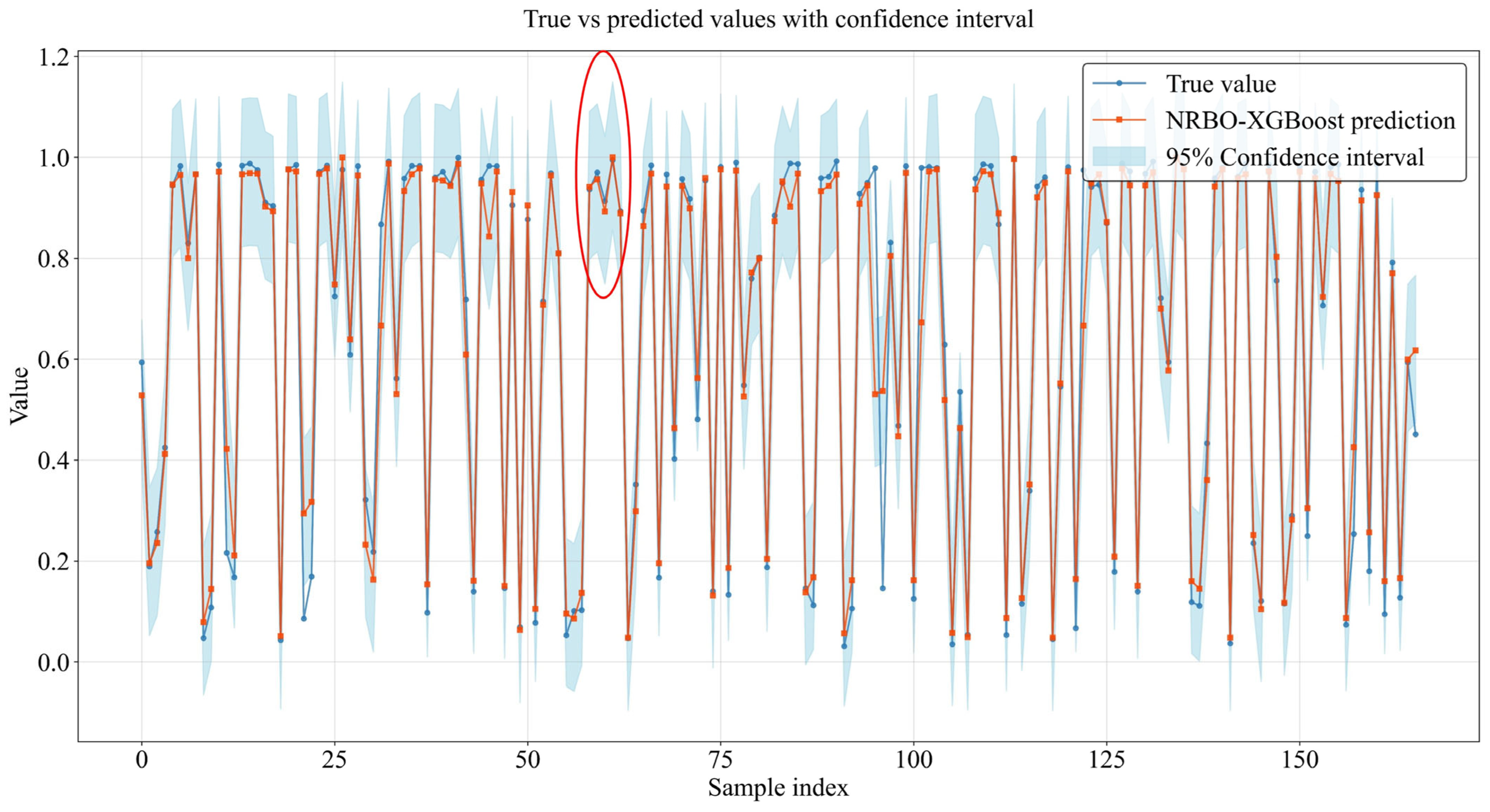
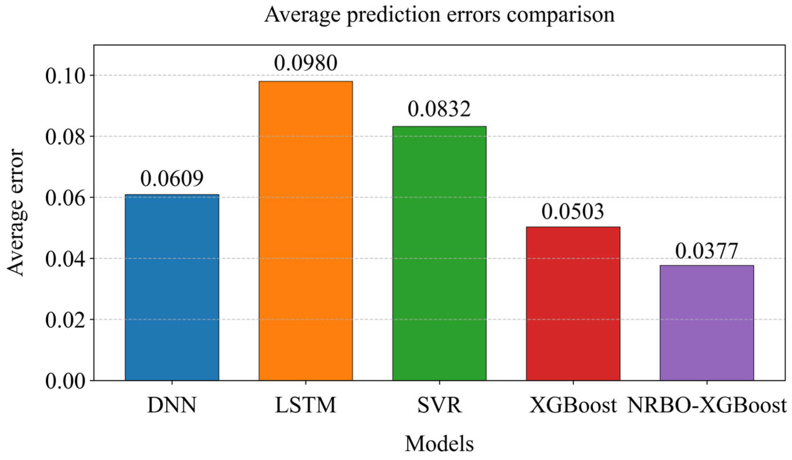
5.3. Results of Model Comparison Experiment

To evaluate the superiority of the NRBO–XGBoost algorithm, four widely used regression prediction algorithms—Deep Neural Network (DNN), Long Short-Term Memory (LSTM) Network, Support Vector Regression (SVR), and the original XGBoost model—were selected as benchmarks. Their hyperparameter configurations are summarized in

Table 4. Hyperparameter configurations for the DNN, LSTM, SVR, and original XGBoost algorithms.

Algorithm	Hyperparameter	Configuration
DNN	Activation function	Relu
	Optimizer	Adam
	Learning rate	0.001
	Batchsize	24
	Dropout ratio	0.1
LSTM	Activation function	data
	Optimizer	Adam
	Learning rate	0.001
	Batchsize	24
	Time step	3
SVR	Kernel function	rbf
	C parameter	1.0
	Gamma parameter	Auto
	Tol parameter	0.001
Original XGBoost	Learning rate	0.1
	Maximum tree depth	4
	Subsampling ratio	0.8
	Column Sampling Ratio	0.8
	Gamma parameter	0.1
	Min child weight	5
	Scale pos weight	1

.

The dataset was trained using the above model and the evaluation metrics of the model were calculated using the validation set; the results obtained are shown in

Table 5. Validation results for the different prediction models.

Algorithm	RMSE	MAE	ED	R2
DNN	0.1231	0.0677	2.1253	0.8828
LSTM	0.1556	0.0948	2.6859	0.8127
SVR	0.1419	0.0908	2.4498	0.8442
XGBoost	0.1069	0.0593	1.8458	0.9116
NRBO–XGBoost	0.0971	0.04619	1.6739	0.9273

.

According to the results in Table 5, XGBoost is already superior to DNN, LSTM, and SVR models in RMSE, MAE, and ED parameters, even when not optimized. The model optimized by the NRBO algorithm achieves the best parameters compared to the other four models. Therefore, the NRBO algorithm can improve the prediction accuracy and generalization performance of the XGBoost algorithm by optimizing in the XGBoost hyperparameter space.

To evaluate the generalization performance of NRBO–XGBoost and the comparative algorithms on unseen data, the five algorithms were independently applied to predict test-set samples. The predicted results were compared to the ground truth values, with 95% confidence intervals employed to quantify prediction accuracy. The corresponding outcomes are illustrated in Figure 17, Figure 18, Figure 19, Figure 20 and Figure 21. Additionally, the mean error between predicted and true values across all algorithms was statistically computed, and these results are visualized as a histogram in Figure 22.

As evidenced by the test results in Figure 17, Figure 18, Figure 19, Figure 20 and Figure 21, the NRBO–XGBoost framework demonstrates superior predictive accuracy compared to benchmark algorithms, with predicted values consistently aligning closer to ground truth measurements. This improvement is particularly evident in certain data regions, as shown by the red circled data points in Figure 17, Figure 18, Figure 19, Figure 20 and Figure 21.

Furthermore, statistical analysis of the prediction errors (Figure 22) reveals that NRBO–XGBoost achieves the lowest mean prediction error, at 0.0377, representing a 61.53% reduction compared to LSTM (0.098) and a 25% improvement over standalone XGBoost (0.0503). The error-distribution histograms further indicate significantly narrower dispersion ranges and reduced outliers, validating the method’s robustness against data heterogeneity.

These experimental results, combined with the algorithm’s previously established convergence stability in high-dimensional spaces (Figure 12), collectively demonstrate its notable advantages in generalization performance and robustness when handling high-dimensional nonlinear data.

6. Conclusions

To improve the adaptability of airborne SAR in complex electromagnetic environments, a laboratory-based EMI test system was established. The methodology constructs a mapping relationship between EMI signals and SAR imaging performance degradation, complemented by a corresponding evaluation framework for interference effects. The experimental findings reveal distinct impact patterns of the various interference signals evident in the SAR image quality. Furthermore, the NRBO algorithm was integrated to optimize XGBoost hyperparameters, resulting in the NRBO–XGBoost model. Trained and validated using datasets from the airborne SAR EMI test system, the model was benchmarked against traditional prediction methods. Four evaluation metrics—RMSE, MAE, ED, and R²—were applied to assess model performance. Finally, the generalization capabilities of competing models were tested using test datasets, leading to the following conclusions:

(1) The interference laws caused by different types of interference signals in the context of airborne SAR are different; these distinctions are mainly related to the type of interference signal, the frequency deviation between the interference signal and the center frequency of the radar, the overlapping bandwidth between the interference signal and the radar working signal frequency band, and the ISR.

(2) By using the NRBO algorithm to optimize the XGBoost hyperparameter space, the prediction accuracy of the XGBoost model can effectively be improved. NRBO–XGBoost can accurately predict the environmental electromagnetic effects resulting in different types and parameters of interference signals in the airborne SAR.

(3) After comparing and analyzing the NRBO–XGBoost prediction model relative to other typical prediction models, the results show that the airborne SAR environmental electromagnetic effect prediction model based on NRBO–XGBoost has higher accuracy and better generalization performance, and can improve the adaptive ability of airborne SAR in the complex electromagnetic environment.

References

1. Gallucci, S.; Fiocchi, S.; Bonato, M.; Chiaramello, E.; Tognola, G.; Parazzini, M. Exposure Assessment to Radiofrequency Electromagnetic Fields in Occupational Military Scenarios: A Review. Int. J. Environ. Res. Public Health 2022, 19, 920. [Google Scholar] [CrossRef] [PubMed]
2. Liu, Q.-F.; Zheng, S.-Q.; Zuo, Y.; Zhang, H.-Q.; Liu, J.-W. Electromagnetic Environment Effects and Protection of Complex Electronic Information Systems. In Proceedings of the IEEE MTT-S International Conference on Numerical Electromagnetic and Multiphysics Modeling and Optimization (NEMO), Beijing, China, 7–9 December 2020. [Google Scholar] [CrossRef]
3. Chen, S.; Yuan, Y.; Wang, S.-X.; Yang, H.; Zhu, L.; Zhang, S.; Zhao, H. Multi-Electromagnetic Jamming Countermeasure for Airborne SAR Based on Maximum SNR Blind Source Separation. IEEE Trans. Geosci. Remote Sens. 2022, 60, 5240211. [Google Scholar] [CrossRef]
4. Tao, M.-L.; Li, J.-S.; Fan, Y.-F.; Su, J.; Wang, L. Effects of Interference on Synthetic Aperture Radar Measurements: An Illustrative Example. In Proceedings of the 2020 XXXIIIrd General Assembly and Scientific Symposium of the International Union of Radio Science (URSI GASS), Rome, Italy, 29 August–5 September 2020. [Google Scholar] [CrossRef]
5. Hu, X.; Shi, J.; Wei, T.; Li, N. An Enhanced Extraction and Mitigation Scheme of Mutual RFI Between Spaceborne SARs Based on Pulse Compression. IEEE Trans. Geosci. Remote Sens. 2025, 63, 5208720. [Google Scholar] [CrossRef]
6. Natsuaki, R.; Jäger, M.; Prats-Iraola, P. Similarity Approach for Radio Frequency Interference Detection and Correction in Multi-Receiver SAR. In Proceedings of the IGARSS 2020—IEEE International Geoscience and Remote Sensing Symposium, Waikoloa, HI, USA, 26 September–2 October 2020. [Google Scholar] [CrossRef]
7. Fang, L.; Zhang, J.; Ran, Y.; Chen, K.; Maidan, A.; Huan, L.; Liao, H. Blind Signal Separation with Deep Residual Networks for Robust Synthetic Aperture Radar Signal Processing in Interference Electromagnetic Environments. Electronics 2025, 14, 1950. [Google Scholar] [CrossRef]
8. Feng, Y.; Han, B.; Wang, X.; Shen, J.; Guan, X.; Ding, H. Self-Supervised Transformers for Unsupervised SAR Complex Interference Detection Using Canny Edge Detector. Remote Sens. 2024, 16, 306. [Google Scholar] [CrossRef]
9. Shen, Y.; Wang, Y.-M.; Ma, L.-Y.; Chen, Y.-Z. Research on Simulation Method for Nonlinear Effects of Airborne SAR EMI. AIP Adv. 2023, 13, 105002. [Google Scholar] [CrossRef]
10. Chen, S.; Lin, Y.; Yuan, Y.; Li, X.; Hou, L. Suppressive Interference Suppression for Airborne SAR Using BSS for Singular Value and Eigenvalue Decomposition Based on Information Entropy. IEEE Trans. Geosci. Remote Sens. 2023, 61, 5205611. [Google Scholar] [CrossRef]
11. Fang, F.-P.; Li, H.-L.; Meng, W.-Z.; Dai, D.; Xing, S. Synthetic-Aperture Radar Radio-Frequency Interference Suppression Based on Regularized Optimization Feature Decomposition Network. Remote Sens. 2024, 16, 2540. [Google Scholar] [CrossRef]
12. Kim, S.; Lee, D.; Park, Y.; Joo, J.; Kim, J.; Kim, J.; Bang, J.-H. Deceptive Jamming for Spaceborne SAR Using Estimated Signal Parameters and Intercepted Signal Phase. IEEE Access 2024, 12, 169388–169403. [Google Scholar] [CrossRef]
13. Guo, X.; Tian, T.; Tan, H.; Fan, W.; Zhou, F. A Deceptive Jamming Technology Against SAR Based on Optical-to-SAR Template Translation. IEEE Trans. Aerosp. Electron. Syst. 2024, 60, 5715–5729. [Google Scholar] [CrossRef]
14. Liu, Z.; Cheng, D.; Li, N.; Min, L.; Guo, Z. Two-Dimensional Precise Controllable Smart Jamming Against SAR via Phase Errors Modulation of Transmitted Signal. IEEE Geosci. Remote Sens. Lett. 2024, 21, 4000705. [Google Scholar] [CrossRef]
15. Liu, G.; Zhang, Q.; Huang, Z.; Chen, T.; Mu, B.; Guo, H. SAR Imaging of Dense False Target Jamming Based on Phase Modulation. IEEE Geosci. Remote Sens. Lett. 2025, 22, 4000105. [Google Scholar] [CrossRef]
16. Hu, H.; Ao, Y.; Bai, Y.; Cheng, R.; Xu, T. An Improved Harris’s Hawks Optimization for SAR Target Recognition and Stock Market Index Prediction. IEEE Access 2020, 8, 65891–65910. [Google Scholar] [CrossRef]
17. Xu, W.; Xing, W.; Fang, C.; Huang, P.; Tan, W. RFI Suppression Based on Linear Prediction in Synthetic Aperture Radar Data. IEEE Geosci. Remote Sens. Lett. 2021, 18, 2127–2131. [Google Scholar] [CrossRef]
18. Huang, M.; Zhao, H.; Chen, Y.-Z. Research on SAR Image Quality Evaluation Method Based on Improved Harris Hawk Optimization Algorithm and XGBoost. Sci. Rep. 2024, 14, 28364. [Google Scholar] [CrossRef]
19. Macchiarulo, V.; Giardina, G.; Milillo, P.; Aktas, Y.D.; Whitworth, M.R.Z. Integrating Post-Event Very High Resolution SAR Imagery and Machine Learning for Building-Level Earthquake Damage Assessment. Bull. Earthq. Eng. 2024, 22, 1–27. [Google Scholar] [CrossRef]
20. Ponmani, E.; Saravanan, P. Image Denoising and Despeckling Methods for SAR Images to Improve Image Enhancement Performance: A Survey. Multimed. Tools Appl. 2021, 80, 26547–26569. [Google Scholar] [CrossRef]
21. Wei, S.-J.; Zhang, H.; Zeng, X.-F.; Zhou, Z.; Shi, J.; Zhang, X. CARNet: An Effective Method for SAR Image Interference Suppression. Int. J. Appl. Earth Obs. Geoinf. 2022, 114, 103019. [Google Scholar] [CrossRef]
22. Liu, S.; Tian, S.; Zhao, Y.; Hu, Q.; Li, B.; Zhang, Y.-D. LG-DBNet: Local and Global Dual-Branch Network for SAR Image Denoising. IEEE Trans. Geosci. Remote Sens. 2024, 62, 5205515. [Google Scholar] [CrossRef]
23. Wang, X.; Wu, Y.; Shi, C.; Yuan, Y.; Zhang, X. ANED-Net: Adaptive Noise Estimation and Despeckling Network for SAR Image. IEEE J. Sel. Top. Appl. Earth Obs. Remote Sens. 2024, 17, 4036–4051. [Google Scholar] [CrossRef]
24. Yang, C.; Li, C.; Zhu, Y. Denoising and Feature Enhancement Network for Target Detection Based on SAR Images. Remote Sens. 2025, 17, 1739. [Google Scholar] [CrossRef]
25. Zhang, Q.; Wang, Y.; Cheng, E.; Ma, L.; Chen, Y. Investigation on the Effect of the B1I Navigation Receiver Under Multifrequency Interference. IEEE Trans. Electromagn. Compat. 2022, 64, 1097–1104. [Google Scholar] [CrossRef]
26. Chen, F.; Huang, L.; Zhou, Q.; Ren, C. GNSS Cognitive Interference Mitigation Method Based on Deep Learning. In Proceedings of the 2024 5th International Conference on Electronic Communication and Artificial Intelligence (ICECAI), Shenzhen, China, 24–26 May 2024. [Google Scholar] [CrossRef]
27. Yang, F.; Zhang, Q.; Yu, H.; Guo, X.; Gong, C. GNSS Interference Suppression for Spacecraft Using Integrated Navigation Based on Support Vector Regression. In Proceedings of the 2024 43rd Chinese Control Conference (CCC), Kunming, China, 25–27 July 2024. [Google Scholar] [CrossRef]
28. Lu, F.; Fan, Z.; Hu, C.; Ma, C.; Chen, Y.; Jiang, H. Deep Reinforcement Learning-Driven Analog Self-Interference Cancellation for LEO Navigation Augmentation Systems. In Proceedings of the 2024 IEEE 24th International Conference on Communication Technology (ICCT), Chengdu, China, 18–20 October 2024. [Google Scholar] [CrossRef]
29. Zhang, D.-X.; Cheng, E.-W.; Wan, H.-J.; Zhou, X.; Chen, Y. Prediction of Electromagnetic Compatibility for Dynamic Datalink of UAV. IEEE Trans. Electromagn. Compat. 2018, 61, 1474–1482. [Google Scholar] [CrossRef]
30. Zhang, X.; Chen, Y.; Zhao, M.; Li, Y. Assessment of EMI Effects on UAV Data Links. IEEE Trans. Electromagn. Compat. 2025, 67, 1–14. [Google Scholar] [CrossRef]
31. Xu, T.; Chen, Y.; Zhao, M.; Wang, Y.; Zhang, X. Adaptive EMS Test Design Method on UAV Data Link Based on Bayesian Optimization. IEEE Trans. Electromagn. Compat. 2023, 65, 716–724. [Google Scholar] [CrossRef]
32. Sowmya, R.; Premkumar, M.; Jangir, P. Newton-Raphson-Based Optimizer: A New Population-Based Metaheuristic Algorithm for Continuous Optimization Problems. Eng. Appl. Artif. Intell. 2024, 128, 107532. [Google Scholar] [CrossRef]
33. Chen, T.-Q.; Guestrin, C. XGBoost: A Scalable Tree Boosting System. In Proceedings of the 22nd ACM SIGKDD International Conference on Knowledge Discovery and Data Mining, San Francisco, CA, USA, 13–17 August 2016. [Google Scholar] [CrossRef]
34. Liu, Y.; Li, J.; Yang, L.; Xu, C. SAR Jamming Effect Evaluation Method Combining Texture Structure Similarity and Image Contour Similarity. Mod. Electron. Tech. 2023, 46, 34–38. [Google Scholar] [CrossRef]
35. Shami, T.M.; El-Saleh, A.A.; Alswaitti, M.; Al-Tashi, Q.; Summakieh, M.A.; Mirjalili, S. Particle Swarm Optimization: A Comprehensive Survey. IEEE Access 2022, 10, 10031–10061. [Google Scholar] [CrossRef]
36. Lambora, A.; Gupta, K.; Chopra, K. Genetic Algorithm—A Literature Review. In Proceedings of the 2019 International Conference on Machine Learning, Big Data, Cloud and Parallel Computing (COMITCon), Faridabad, India, 14–16 February 2019; pp. 380–384. [Google Scholar] [CrossRef]
37. Bilal; Pant, M.; Zaheer, H.; Garcia-Hernandez, L.; Abraham, A. Differential Evolution: A Review of More than Two Decades of Research. Eng. Appl. Artif. Intell. 2020, 90, 103479. [Google Scholar] [CrossRef]
38. Mirjalili, S.; Mirjalili, S.M.; Lewis, A. Grey Wolf Optimizer. Adv. Eng. Softw. 2014, 69, 46–61. [Google Scholar] [CrossRef]
39. Heidari, A.A.; Mirjalili, S.; Faris, H.; Aljarah, I.; Mafarja, M.; Chen, H. Harris Hawks Optimization: Algorithm and Applications. Future Gener. Comput. Syst. 2019, 97, 849–872. [Google Scholar] [CrossRef]
40. Ahmadianfar, I.; Bozorg-Haddad, O.; Chu, X. Gradient-Based Optimizer: A New Metaheuristic Optimization Algorithm. Inf. Sci. 2020, 540, 131–159. [Google Scholar] [CrossRef]
41. Chaves, A.A.; Resende, M.G.C.; Schuetz, M.J.A.; Brubaker, J.K.; Katzgraber, H.G.; de Ar-ruda, E.F.; Silva, R.M.A. A Random-Key Optimizer for Combinatorial Optimization. arXiv 2024, arXiv:2411.04293. [Google Scholar] [CrossRef]
42. Faramarzi, A.; Heidarinejad, M.; Stephens, B.; Mirjalini, S. Equilibrium Optimizer: A Novel Optimization Algorithm. Knowl. Based Syst. 2020, 191, 105190. [Google Scholar] [CrossRef]
Figure 1. Overall framework of the airborne SAR EMI test system.
Electronics 14 02202 g001
Figure 2. Implementation process for the SAR echo inversion technology based on image scenes.
Electronics 14 02202 g002
Figure 3. Imaging results generated by the SAR EMI testing system without interference.
Electronics 14 02202 g003
Figure 4. SAR imaging results with different interference signals: (a) interference result for SFCW; (b) interference result for noise; and (c) interference result for LFMCW.
Electronics 14 02202 g004
Figure 5. The relationship between SAR image interference evaluation factor and frequency under single-frequency continuous wave interference at different frequencies.
Electronics 14 02202 g005
Figure 6. The variation in SAR image interference evaluation factor with noise interference frequency under the same ISR conditions.
Electronics 14 02202 g006
Figure 7. The variation in the SAR image interference evaluation factor, with noise interference at interleaved bandwidths, under the same ISR conditions.
Electronics 14 02202 g007
Figure 8. The variation law for the SAR image interference evaluation factor with LFMCW interference signals of varying frequency, under identical ISR conditions.
Electronics 14 02202 g008
Figure 9. The variation in the interference evaluation factor of the SAR image with the overlapping frequency bands of LFMCW signal and radar working signal, under identical ISR conditions.
Electronics 14 02202 g009
Figure 10. Flowchart for optimizing hyperparameters of XGBoost model using NRBO algorithm.
Electronics 14 02202 g010
Figure 11. Comparison of dataset distribution: (a) distribution of interference types in the training set; (b) distribution of interference types in the test set; (c) distribution of ISR and delta_f parameters in the training set; and (d) distribution of ISR and delta_f parameters in the test set.
Electronics 14 02202 g011
Figure 12. Convergence curve of the NRBO algorithm.
Electronics 14 02202 g012
Figure 13. Comparison diagram of test-set prediction results and true values.
Electronics 14 02202 g013
Figure 14. Validation set and truth value regression fitting effect chart.
Electronics 14 02202 g014
Figure 15. Prediction error between the predicted value and the true value of the validation set.
Electronics 14 02202 g015
Figure 16. Histogram distribution of model prediction error.
Electronics 14 02202 g016
Figure 17. The prediction results of the DNN algorithm on the prediction set.
Electronics 14 02202 g017
Figure 18. The prediction results of the LSTM algorithm on the prediction set.
Electronics 14 02202 g018
Figure 19. The prediction results of the SVR algorithm on the prediction set.
Electronics 14 02202 g019
Figure 20. The prediction results of the XGBoost algorithm on the prediction set.
Electronics 14 02202 g020
Figure 21. The prediction results of the NRBO–XGBoost algorithm on the prediction set.
Electronics 14 02202 g021
Figure 22. The average prediction errors of the different prediction algorithms on the test set.
Electronics 14 02202 g022