Abstract
Herein, to address the challenges faced by Automatic Guided Vehicles (AGVs) in construction site environments, including heavy vehicle loads, extensive road search areas, and randomly distributed obstacles, this paper presents a hierarchical trajectory planning algorithm that combines coarse planning and precise planning. In the first-level coarse planning, lateral and longitudinal sampling is performed based on road environment constraints. A multi-criteria cost function is designed, taking into account factors such as deviation from the road centerline, shortest path cost, and obstacle collision safety cost. An efficient dynamic programming algorithm is used to obtain the optimal path. Considering nonholonomic constraints of vehicles, eliminating inflection points using improved B-Spline path fitting, and a quadratic programming algorithm is proposed to enhance path smoothness, completing the coarse planning algorithm. In the second-level precise planning, the coarse planning path is used as a reference line, and small-range sampling is conducted based on AGV motion constraints, including lateral displacement and longitudinal velocity. Lateral and longitudinal polynomials are constructed. To address the impact of randomly appearing obstacles on vehicle stability and safety, an evaluation function is designed, considering factors such as jerk and acceleration. The optimal trajectory is determined through collision detection, ensuring both safe obstacle avoidance and AGV smoothness. Experimental results demonstrate the effectiveness of this method in solving the path planning challenges faced by AGVs in construction site environments characterized by heavy vehicle loads, extensive road search areas, and randomly distributed obstacles.
1. Introduction
Automatic Guided Vehicles (AGVs) are autonomous navigation devices driven by planning algorithms [,,,]. In recent years, in the construction site environment, AGVs have demonstrated their autonomy and have been used to replace manual labor for flexible material transportation tasks, resulting in cost savings and improved work efficiency [,,]. However, the challenges of heavy vehicle loads, extensive road search areas, and randomly appearing obstacles in construction sites have presented new hurdles for AGV applications in this context, prompting researchers to focus more on path planning techniques tailored to construction site environments [,].
Path planning technology is a method that plans an optimal path based on given target point positions and road conditions [,,,]. By reviewing the research on path planning algorithms in new scenarios of road in recent years, two main research approaches have been summarized. Firstly, combining two or more path planning algorithms, leveraging the strengths of each algorithm, to design path planning algorithms tailored to specific scenarios [,,]. For instance, in reference [], a global path planning algorithm based on an improved A* algorithm and a local path planning algorithm based on an improved artificial potential field algorithm were proposed, achieving theoretical validation for precise obstacle avoidance and rapid navigation of indoor mobile robots. Secondly, by improving a known algorithm and designing heuristic functions, cost functions, etc., tailored to specific scenarios to achieve effective planning results [,,,]. For example, in reference [], a Target-Optimized JPS algorithm was introduced, which constructs search direction priorities based on target point direction vectors and also improves the cost function to obtain shorter paths, reducing computation time.
Dynamic programming techniques based on the greedy approach are well-suited for path planning on large, wide roads [,,]. For example, in reference [], a solution was proposed that uses dynamic programming to inspire continuous state spaces and obtain globally optimal path planning. In reference [], a static obstacle avoidance algorithm based on a grid map was introduced, generating feasible paths by considering the weight of each obstacle and then optimizing these feasible paths through dynamic programming to find several shortest paths. However, these dynamic programming solutions solely focus on finding the shortest path and do not consider the high load conditions of AGVs, resulting in paths without speed information. On the other hand, Frenet sampling planning decouples the lateral and longitudinal aspects of planning and includes speed information in the planned trajectory [,,]. As shown in reference [], it uses the global planning path as a reference line and decouples the local trajectory in the Frenet coordinate system both horizontally and vertically. By considering the designed endpoint sampling rules and taking speed planning into account, it finds the optimal trajectory. However, this method has a higher sampling cost in wide road scenarios.
After analyzing the aforementioned works, it was observed that there are currently very few path planning algorithms specifically designed for construction site environments. Existing algorithms struggle to balance high-speed calculation and extensive sampling range. Therefore, this paper proposes a hierarchical trajectory planning method that integrates road environment constraint sampling (coarse planning) and AGV motion constraint sampling (precise planning). This approach leverages the respective strengths of coarse planning and precise planning and tailored to the specific environment of construction sites, designs cost functions.
The rest of this paper is organized as follows. Section 2 introduces the coarse planning method based on road environment constraint sampling. Section 3 discusses the precise planning algorithm based on motion constraint sampling, and its integration with the coarse planning algorithm to form a hierarchical trajectory planning algorithm. Section 4 conducts experimental tests and data analysis to verify the practical effectiveness and feasibility of the algorithm. Section 5 provides an overall summary.
2. Coarse Planning Algorithm
In the construction site environment, the extensive road search area requires the collection of a large amount of data for both lateral and longitudinal sampling, creating a significant computational burden. To address the challenge of enabling AGVs to quickly compute an accurate, safe, and efficient planning path, this section introduces a dynamic programming algorithm based on the greedy approach. By considering safety, shortest path, and other metrics, a multi-objective evaluation function is designed to efficiently obtain the optimal path. Nonholonomic vehicle constraints are also taken into account, with interpolation at the starting and ending points and the use of the B-Spline algorithm to fit the optimal path and eliminate sharp turns. Given the high load of AGVs, which requires road smoothness, the fitted path is further improved through quadratic programming.
2.1. Lateral and Longitudinal Sampling under Road Environment Constraints
The sampling for coarse planning is based on the S-L coordinate system of the road, with road environment constraints taken into account. It considers road boundaries, the size and positions of obstacles, and the road centerline for sampling. Laterally, uniformly distributed sampling points from the road’s centerline towards both sides at a fixed interval of until reaching the road boundary La. Longitudinally, it uniformly distributes sampling points along the road centerline with a fixed , setting a fixed sampling length Sa. Sampling points are filtered based on the size and position of obstacles, using the obstacle’s center point as the origin and extending outward by dobs to remove sampling points near the obstacle, improving search efficiency. In scenarios with multiple obstacles, this sampling method significantly reduces computational complexity. Additionally, before planning, if it is determined that there are no available sampling points in the s-direction due to obstacles, it can quickly identify an impassable path and initiate a stopping operation, thus enhancing the safety of the AGV. The specific sampling process is illustrated in the following figure (Figure 1). The blue points represent the sampling points, and the red point represents the target points.
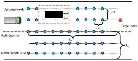
Figure 1.
Sampling based on road environment constraints.
2.2. Selecting the Optimal Path
Traditional dynamic programming algorithms focus solely on finding the shortest path []. However, in the construction site environment, we besides considering path length, it is essential to take into account the influence of obstacles in the construction site and keep the path as close to the road centerline as possible. Then we can accurately assess the cost between two nodes. This paper proposes a multi-objective evaluation function to evaluate the cost between nodes. In addition to the cost of the shortest path, we introduce costs related to deviation from the reference line and obstacle collision safety. These three aspects are considered to provide a diversified evaluation of a path. The implementation method is as follows.
Linear interpolation is performed between two points on adjacent s-layers to obtain several interpolated points. The cost of the shortest path is determined by calculating the cumulative distance between all interpolated points on the s-layers, providing the length cost of the planned path. The cost of deviation from the reference line is characterized by the cumulative sum of values of all interpolated points, taking advantage of the properties of the Frenet coordinate system. For obstacle safety cost, a segmented calculation approach is employed. If the distance between the planning point and the obstacle is greater than 2 m, it is considered sufficiently safe, and no cost is calculated. If the distance is less than 0.5 m, it is considered impassable, resulting in an infinite cost. If the distance falls within the range of 0.5 m to 2 m, the cost is represented by the sum of the squared distances between the interpolated points and the obstacle.
Given the coordinates of interpolated points between two points as and the coordinates of obstacles as the cost equation for the path between these two points is calculated as follows:
where represents the cost associated with the shortest path, represents the cost associated with deviation from the reference line, represents the cost associated with ensuring safety against collisions with obstacles, and represents the distance of the ith point from the nearest obstacle. is an increasing function, and we are more concerned about the final operating state of the vehicle. Therefore, the proportion of trajectory points at the beginning of the planning is not as high as near the endpoint.
As shown in the Figure 2a, each sampling point represents a node, and nodes with the same s-coordinate are grouped into the same layer. Starting from the last layer, we traverse all the points sampled in the l-direction for the same s layer, recording the minimum cost value for each point to reach the endpoint after visiting all points in the next layer in the s-direction. The cost equation is as follows:
where represents the cost from the current node to the next-level target point, and represents the minimum cost from the next-level node to the endpoint.
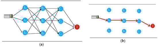
Figure 2.
Optimal path selection based on greedy algorithm principles. (a) Path Searching Based on Greedy Algorithm Principles. (b) Optimal Path.
It continues until reaching the first layer in the s-direction, finding the optimal path with the minimum cost for the vehicle to reach point D, as shown in Figure 2b.
2.3. Curve Fitting and Optimization
As shown in Figure 3a below, in order to ensure planning efficiency, the chosen values of and in dynamic programming cannot be excessively small. This results in relatively large spacing between the output path points generated by the algorithm. Consequently, the planned path often exhibits significant inflection points, lacking the desired smoothness. Thus, the resultant path is typically composed of line segments.
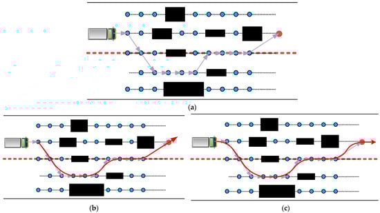
Figure 3.
Comparison of fitting effects. (a) Unfitted. (b) Traditional Fitting. (c) B-Spline Fitting after Interpolation.
We certainly find it imperative to engage in curve fitting. However, if we exclusively apply curve fitting solely to the sampled points, we overlook the non-holonomic constraints posed by the initial and final velocity directions of the AGV. Consequently, while the fitted curve adeptly mitigates the issue of inflection points, it falls short of ensuring that the vehicle’s velocity direction aligns with the planned trajectory direction upon reaching the endpoint. Alternatively, at the starting point, the vehicle may encounter challenges in tracking the planned curve due to velocity direction issues, as depicted in Figure 3b below.
Utilizing the fitting characteristics of B-Splines, this paper proposes a method that, while adhering to the traditional properties of B-Spline fitting, interpolates the coarse planning path to ensure that the tangent direction at the start point of the planned path aligns with the initial velocity direction of the vehicle, and the tangent direction at the end point matches the terminal velocity direction of the vehicle, as shown in the following Figure 3c.
As depicted in Figure 4, the blue points are selected based on the multi-objective evaluation function, the yellow points are interpolation points, and the red points is the endpoints. Since the starting point of the B-Spline fitting curve lies on the line connecting the first and second sampled points and is tangent to that line, to ensure that the tangent direction at the starting point of the B-Spline fitted curve aligns with the vehicle’s velocity direction, a new virtual starting sample point, denoted as 1.1, is inserted after sample point 1. The insertion is made at a distance of . Similarly, to ensure that the tangent direction at the endpoint of the fitted B-Spline curve corresponds to the vehicle’s final velocity direction, a new virtual endpoint sample point, denoted as N.1, is inserted before the last sample point. This insertion is made at a distance of along the extension of the vehicle’s final velocity direction. The B-Spline fitted curve’s endpoint lies on the line connecting the last sample point and the second-to-last sample point and is tangential to that line.
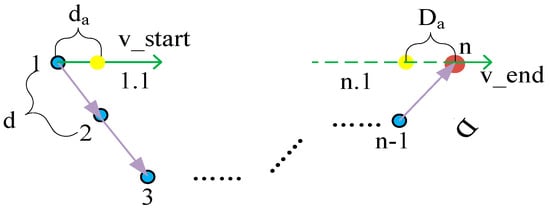
Figure 4.
Improved B-Spline interpolation.
The equation for calculating and are as follows:
where represents the distance between sample points 1 and 2, represents the distance between sample points n − 1 and n. and are interpolation weighting coefficients.
To ensure the quality of the fitted curve while considering the velocity direction, it is important to choose appropriate values for and . Taking the interpolation position of n.1 as an example, as illustrated in Figure 5, different values of can result in significant differences in the fitting performance. Factors such as the alignment of the fitted curve with the original path points, the length of the fitted curve, and its smoothness vary with different values of . Therefore, it is necessary to determine the optimal values for and to ensure the best fitting results.
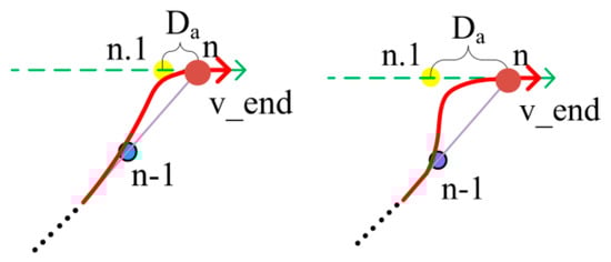
Figure 5.
The fitting effect of different n2.
As Section 2.1 involved the filtering of sampling points close to obstacles based on road environment sampling, and Section 2.2 considered obstacle distance as one of the cost functions for optimal path planning, there is no need to consider the obstacle cost function in the small-scale optimization during curve fitting. In contrast, our primary focus is on the smoothness, shortest path, and alignment with sampling points of the planned path. Therefore, considering the original coordinates as and the optimized coordinates as we can improve Equation (2) as follows:
where represents the smoothness cost, represents the length cost, and represents the deviation cost relative to the original points. , , and are cost coefficients.
The value ranges for and are defined as follows:
By traversing and at different values in Equation (5), the cost calculated according to Equation (4) will be obtained. The optimal values for and will be selected based on the minimum cost value. After obtaining the best and , the entire path from the coarse planning phase will undergo quadratic programming using the same parameter criteria as defined in Equation (4).
The variable set P representing the entire path is defined as follows:
Based on Equations (4) and (6), the expressions for the smoothness cost , length cost , and similarity cost can be derived as follows:
With the above derivations, the cost function can be modified as follows:
The quadratic programming equation is as follows:
Combining Equations (7)–(9), we can obtain:
To prevent excessive impact on the B-spline fitting due to the quadratic programming, interval tolerances are introduced. The tolerance set B is defined as follows:
This is performed to prevent the quadratic programming from adversely affecting the fitting of the improved B-spline. With this, Equations (6)–(11) are incorporated into the quadratic programming solver for iterative solution, yielding the optimal coarse planning path.
3. Precise Planning Algorithm
The coarse planning phase is used to obtain a high-quality planning path with relatively low computational resources. However, the planned path does not include velocity information. In construction environments, AGVs often carry heavy loads, and planning without velocity information can be highly dangerous under high-load conditions. Additionally, the B-Spline fitting and quadratic optimization used in coarse planning make minor adjustments to the path points obtained from dynamic planning. Therefore, collision safety detection is still necessary. In this section, we propose a precise planning algorithm based on the results of coarse planning. This algorithm uses the coarse planning results as a reference line and samples in the longitudinal direction based on velocity and in the lateral direction based on lateral displacement. It considers additional factors like jerk to ensure the smoothness of AGV motion under velocity planning. Moreover, it includes collision detection to achieve a safe and high-quality trajectory planning solution. Implementing the precise algorithm on the basis of coarse planning significantly reduces the sampling count, thereby addressing the drawback of high computational load associated with precise planning.
3.1. Construction of Trajectory Polynomials under Motion Constraint Sampling
In the Frenet coordinate system, the planning problem involves a total of three dimensions, namely (s, d, t). This high-dimensional optimization problem can be decoupled into two independent optimization problems in the lateral (d, t) and longitudinal (s, t) directions, which are sampled and processed separately.
In accordance with the hardware specifications, environmental constraints, safety considerations, and other factors related to the AGV, there are boundary constraints on the lateral displacement (d), velocity (v), acceleration (a), jerk (j), and planned curvature (k). The lateral and longitudinal sampling must adhere to the following motion constraints.
Lateral sampling involves the vehicle starting from the reference line and sampling on both sides of the vehicle at intervals of while adhering to the motion constraints defined in Equation (12). This process continues until sampling reaches the road boundary. After completing this lateral sampling, the next step is to sample in the time domain with intervals of . When the sampling point , initial time , and planning time are determined, a fifth-degree polynomial is constructed for the relationship between time () and lateral displacement () as follows:
The fifth-degree polynomial for lateral sampling can be solved given the known initial position , final position and time instants and .
Under the conditions specified in Equation (12), the longitudinal (s) sampling is slightly different. Instead of using for longitudinal sampling, it uses a given target velocity . Setting with as the reference and sampling velocities on both sides to obtain v can be expressed as follows:
Subsequently, time is sampled at intervals of . Upon completing the sampling of both velocity and time, it is tantamount to having accomplished the sampling of . The advantage of this approach is that, since the sampled values represent velocities, it facilitates the planning of velocity profiles. Consequently, a quartic polynomial concerning velocity and time is constructed as follows.
Analogous to lateral sampling planning, this quartic polynomial can be resolved, thereby concluding the solution process for the current planning iteration.
Upon the resolution of both lateral and velocity sampling polynomials, an assortment of trajectories is generated through the permutation and combination of each lateral sampling and longitudinal velocity sampling under the same planning timeframe. The series of trajectory clusters generated by sampling are shown in the following figure (Figure 6). The dark blue line represents the centerline of the road, the purple line represents the sampling trajectory, and the green points represent the trajectory points selected for planning.
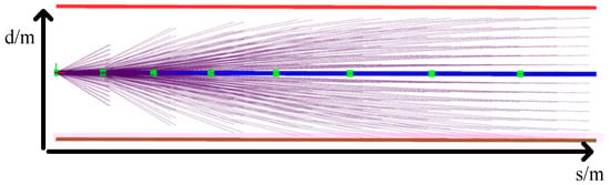
Figure 6.
Trajectory cluster.
3.2. Selection of the Optimal Trajectory
The evaluation function for precise planning is set up from three aspects, driving stability, conformity with the reference line, and convergence effect of the desired speed. Paths with potential collision risks are excluded through collision detection, thus obtaining the Optimal Trajectory. Driving stability is characterized by the absolute values of the longitudinal and lateral jerk throughout the vehicle’s planned trajectory, ensuring that high-load AGVs can smoothly operate while avoiding obstacles at construction sites or during acceleration and deceleration. The degree of conformity to the desired path is represented by the absolute value of the d-coordinate in the Frenet frame of the planned path points, aiming to align the AGV as closely as possible with the desired path tracking. The convergence effect on the desired speed is represented by the squared difference between the planned speed and the desired speed, ensuring that the vehicle can converge to the desired speed relatively quickly. The specific calculation equation is as follows:
where represents the cost of stability, represents the cost of conformity with the desired path, and represents the cost of conformity with the desired speed.
The calculation equation is as follows (, , and as cost coefficients).
During actual testing, it was observed that when facing obstacles at construction sites, the vehicle might frequently encounter situations where it is positioned between two trajectories with similar costs. This leads to frequent replanning of the vehicle’s trajectory, resulting in variability in the trajectory planning and causing instability in the vehicle’s movement, as illustrated in the following Figure 7. Due to similar costs, the AGV may frequently switch optimal trajectories among the following three trajectories.
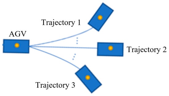
Figure 7.
Frequent alteration of trajectory planning.
To address this phenomenon, a new cost function is introduced as follows:
where represents the similarity between the starting point of the current planned path and that of the previous frame’s planned path.
Under the premise that other paths do not significantly differ from the previous frame’s planned path, to ensure vehicular stability, a preference is given to planning results similar to the previous frame’s plan. This approach effectively circumvents the issue of repetitive planning for AGVs under critical cost function scenarios. Consequently, the comprehensive evaluation equation for precise planning is as follows.
Although the coarse planning algorithm considers obstacle distances and sets a safe distance, to prevent minor adjustments in the planned trajectory due to curve fitting in Section 2.3 and precise planning in Section 3.1, collision detection is still necessary to ensure the safety of the trajectory. All trajectories are sorted from lowest to highest cost according to Equation (18). The obstacle collision detection starts with the trajectory having the lowest cost, and the detection process is illustrated in the following figure (Figure 8). The black rectangle represents obstacles, and the red circle represents the minimum circumscribed circle of obstacles.
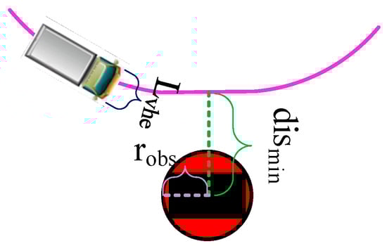
Figure 8.
Collision detection.
By iterating through all points of the trajectory output from the precise planning process, the trajectory point closest to the obstacle is identified, and the minimum distance is calculated. Based on the dimensions of the obstacle obtained from the perception module, the minimum circumscribed circle radius of the obstacle is determined. represents the width of the vehicle’s front. A trajectory is deemed safe if it satisfies the following condition; otherwise, the next trajectory is examined. The safety determination condition is as follows:
If the trajectory is found to be free of collisions with obstacles, it is selected and outputted. Otherwise, the next trajectory is examined until a suitable one is identified. If no trajectory meets the safety requirements, the vehicle will stop and trigger an alarm.
3.3. The Hierarchical Trajectory Planning Algorithm Based on Coarse and Precise Planning
Section 2 describes a coarse planning algorithm based on a greedy approach. Although it is computationally simple and efficient, ensuring smooth path processing, this algorithm does not take into account velocity planning. In construction site environments, where obstacles may appear randomly, the absence of velocity planning is considerably unsafe. High-load AGVs must consider the impact of changes in velocity.
The precise planning algorithm described in this chapter, while incorporating velocity planning, still requires a substantial amount of sampling calculations for wide roads and larger environments at construction sites. It necessitates frequent construction and solving of quintic and quartic polynomials. Moreover, the decoupled lateral and longitudinal planning, coupled through time, demands permutation and combination, resulting in a significant computational load.
This paper proposes a hierarchical trajectory planning algorithm for construction sites, and the specific implementation process is as follows:
- (1)
- According to Section 2.1, under road environmental constraints, starting from the centerline of the road, a smaller Δs and Δl for sampling, remove unnecessary sampling points based on obstacles to improve sampling efficiency.
- (2)
- According to Section 2.2, consider the cost of path length, obstacle collision safety, and deviation from the reference line to calculate the cost function between nodes in adjacent columns. Then, based on greedy thinking, find the optimal path.
- (3)
- According to Section 2.3, the optimal path point is fitted and optimized. Using the improved B-Spline for fitting, eliminate inflection points while considering the non-holonomic constraints of the VGA at the starting and ending points. A quadratic programming equation is constructed considering smoothness, shortest path, and similarity with the original path. Then, the coarse planning has been completed as shown in Figure 9.
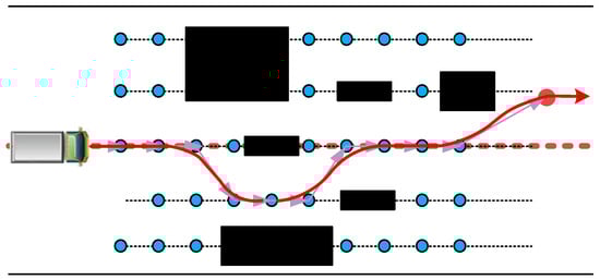 Figure 9. Coarse planning.
 - (4)
- According to Section 3.1, horizontal and vertical sampling are carried out based on the motion constraints of AGV, and lateral fifth and horizontal fourth degree polynomials are constructed separately. The reference line of the second layer planning algorithm no longer uses the road centerline as the reference line but uses the result of coarse planning as the reference line. A smaller sampling width L is used to perform small-scale horizontal sampling on the results of coarse planning. Combine horizontal and lateral trajectories at the same sampling time to form trajectory bundles.
- (5)
- According to Section 3.2, from driving stability, conformity with the reference line, the rate of convergence from the expected speed and the degree of conformity with the previous trajectory is used to calculate the cost for each trajectory. Starting from the trajectory with the lowest cost, collision detection is performed sequentially. Output is the trajectory with the lowest cost and satisfying collision detection. Then, the Precise planning algorithm has been completed as shown in Figure 10 (The blue line represents the sampling boundary, the red line represents the result of coase planning as a reference line).
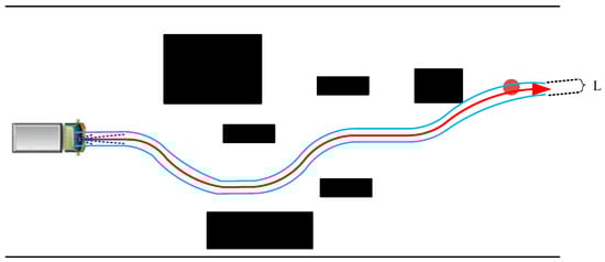 Figure 10. Precise planning.
The hierarchical planning algorithm process is depicted in the Figure 11.
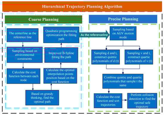
Figure 11.
Algorithm flowchart.
In terms of operational efficiency, coarse planning utilizes the idea of greedy algorithms, reducing the time complexity from in traditional dynamic programming algorithms to Precise planning relies on the rough solutions of coarse planning, with only a number of three to five horizontal samples. Therefore, the time complexity of precise planning is reduced from to , resulting in a time complexity of for the entire hierarchical planning algorithm. It can meet the demand for algorithm efficiency for the wide road area in the construction site environment.
In terms of safety, the sampling points near obstacles are filtered in Section 2.1. As shown in Equation (1) of Section 2.2, the cost function of coarse planning requires the planned trajectory to be far away from obstacles and set a minimum distance of 0.5 m. The collision detection conducted in Section 3.2 prevents potential safety hazards due to the curve fitting optimization in Section 2.3, ensuring the safety of the planned path.
In terms of trajectory smoothness, the improved B-spline fitting takes into account the non-holonomic constraints of AGV, eliminates trajectory inflection points and smooths and optimizes the path through quadratic programming. And precise planning ultimately obtains a smooth trajectory based on indicators such as lateral and longitudinal jerk.
4. Experimental Validation
In this section, experiments were conducted using an AGV built by Weihai Tiante Intelligent Technology Co., Ltd. (Weihai, China) as the experimental platform, as shown in Figure 12. The exact specifications of the AGV are presented in Table 1. Consequently, the velocity planning range should be within 0 to 1.5 (m/s), while the maximum curvature allowed is specified as 1 m−1.
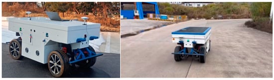
Figure 12.
AGV.

Table 1.
The exact specifications of the AGV.
The experiments were carried out in the construction site environment at Guangzhou Baiyun Airport, as shown in the following figure. The operating road within this environment constitutes a temporary or semi-permanent structure. The width of the road is typically ranging from 6 to 10 m or wider. In the experiment, the boxes were used to simulate the obstacles encountered by AGV, as shown in the following figure (Figure 13).
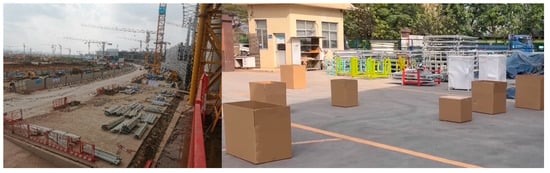
Figure 13.
Experimental environment and obstacles.
Experiments involved variations in vehicle positions, target point locations, initial velocities, target velocities, and other parameters. These experiments were designed to test and validate the effectiveness of the hierarchical planning proposed in this paper. The stability and reliability of the algorithm was also verified. Representative experimental results were selected for detailed analysis and illustration.
4.1. Experimental System
As shown in Figure 14, Figure 15, Figure 16 and Figure 17. The industrial computer used in this experiment is the NVIDIA AGX Orin 64G. The depth camera (Stereolabs Technologies Inc., San Francisco, CA, USA; Beijing, China) was employed as the obstacle perception sensor, while a laser radar (DJI, Shenzhen, China) and INS570D inertial navigation components (Guangdong Daoyuan Electronic Technology Co., Guangzhou, China) served as localization sensors. These sensors were chosen for experimental testing of the planning algorithm in this paper, under the condition that the perception algorithms meet all the requirements of the experiment.
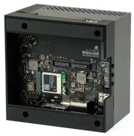
Figure 14.
JETSON AGX ORIN.
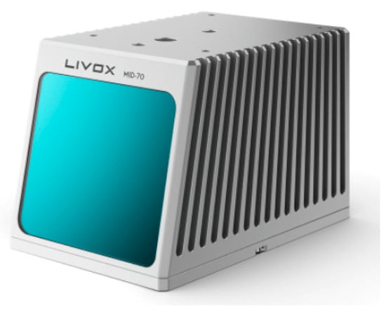
Figure 15.
Livox-MID-70.

Figure 16.
ZED.
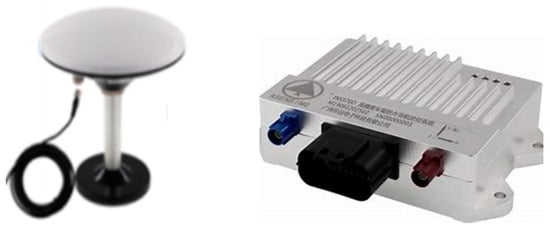
Figure 17.
INS570D.
Detailed information about industrial computers and sensors are shown in the tables below (Table 2, Table 3, Table 4 and Table 5).
Table 2.
JETSON AGX ORIN information.
Table 3.
Livox-MID-70 information.
Table 4.
ZED information.
Table 5.
NS570D information.
As shown in Figure 18, the INS570D module, the Livox-MID-70 and the ZED, respectively, communicate with the industrial computer through the RS485 serial port, the Ether Net, and the USB 3.0. The industrial computer runs the perception and planning algorithm, sends the motion commands to the AGV through the Controller Area Network (CAN).
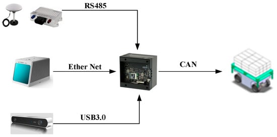
Figure 18.
Device communication.
As shown in Figure 19 there are four ZED cameras installed around the AGV, a LiDAR is installed before and after the AGV, and two are installed on each side. The industrial computer and INSS570D are integrated inside the AGV, and the INS570D antenna is placed diagonally in front and behind the AGV.
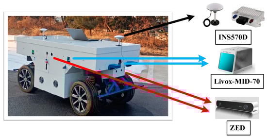
Figure 19.
Device installation.
The sensors used in the perception system in this paper (including ZED, LiDAR, inertial navigation, etc.) were pre calibrated using their official calibration methods and procedures before the experiment. Please refer to the official websites of each sensor for details. During the experiment, a large number of tests have shown that the accuracy of obstacle recognition and positioning can reach the centimeter level.
4.2. AGV Tracking Control for Experiments
The kinematic model of AGV is shown in the Figure 20. AGV is a four-wheel steering model, which regards all movements of AGV to be considered as circular movements around point O’ on the plane of the AGV body. Linear motion and spin are its special limiting motion states. When all components of the AGV, including the wheels, move in a circular motion around a certain point, the angular velocity is the same, and the linear velocity is perpendicular to the center of the circle. We set the wheelbase of the AGV to and the wheel-base to , The speeds of the four drive motors are , The angle of the four steering motors are , . The angle between AGV speed and is δ. The turning radii of the four wheels are ,. The turning radius of AGV is .
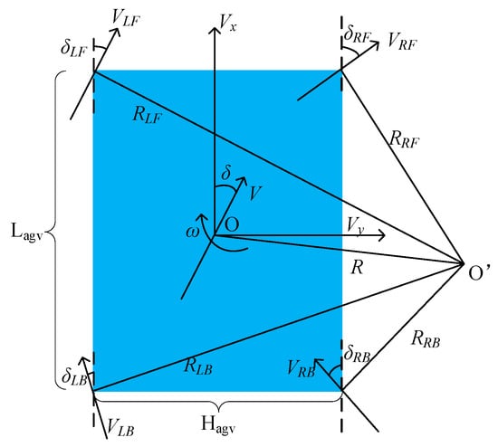
Figure 20.
AGV kinematic model.
The , can be obtained according to the following equation after obtaining the and .
Then, the , can be calculated according to the following equation.
Then, , can be obtained according to .
According to the following equation, , can be obtained
At this point, we have achieved the kinematic solution of the AGV, and based on and , we can obtain , , .
After obtaining the optimal trajectory in Section 3.3, the trajectory is composed of a set of points with speed information. By traversing the trajectory points with positioning information, we find the closest trajectory point to AGV, set the preview distance to be . We find the target point. The angle deviation between AGV and target point is .
where , are the coordinates of the target point. are the coordinates of AGV, is the heading of AGV.
Using PD control to calculate the .
where are the PID parameters, and is the previous angle error.
The target point is equipped with speed information , the current speed () of AGV can be obtained through the perceived information, the difference between the two results in a speed deviation is the , then the speed control is using an incremental PID algorithm as shown in the following equation:
where are the PID parameters, and is the previous speed error.
According to the Equations (26) and (27), we calculate the and , respectively, to control AGV.
The parameters used in the control are shown in the table below (Table 6).
Table 6.
Control parameters.
4.3. Verification of Selection of Optimal Path in Coarse Planning
In the real road environment at the construction site, sampling was performed based on constraints such as road boundaries, obstacles, and reference lines. Over 30 sets of parallel experiments were conducted with different start and end points to validate the performance of the multi-objective evaluation function in coarse planning. Finally, three representative sets of experiments were selected for presentation. Test 1 is the starting point located on the centerline of the road, and the endpoint is also located on the centerline of the road. Test 2 is the starting point located away from the centerline of the road, and the endpoint is also located away from the centerline of the road. Test 3 starts at the center of the road and ends far away from the center of the road and near obstacles. By setting different conditions, we fully verify the reliability of the planning algorithm. The parameter values during the experiments are listed in Table 7.
Table 7.
Sampling and multi-objective evaluation function parameters.
The experimental results are presented in the following figures (Figure 21, Figure 22 and Figure 23). Blue arrows indicate the current pose of the vehicle, brown rectangles represent obstacles, green squares represent obstacle safety distances, blue dots represent sampling points, red dots represent the output points from coarse planning, and red arrows indicate the vehicle’s target endpoint.
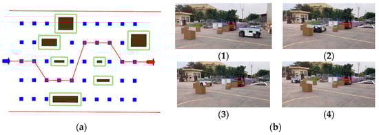
Figure 21.
Effectiveness of Coarse Planning in test 1. (a) Display on the host computer in test 1. (b) (1)–(4) are the testing process at the corresponding real site in test 1.
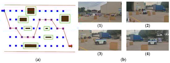
Figure 22.
Effectiveness of coarse planning in test 2. (a) Display on the host computer in test 2. (b) (1)–(4) are the testing process at the corresponding real site in test 2.
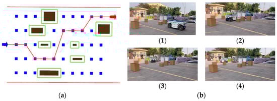
Figure 23.
Effectiveness of coarse planning in test 3. (a) Display on the host computer in test 3. (b) (1)–(4) are the testing process at the corresponding real site in test 3.
Based on the experimental results, we can obtain the following conclusions.
(1) Sampling based on environmental constraints efficiently and succinctly achieved waypoint sampling. In the experiment, a total of 50 points were sampled to cover a width of 8 m and extended longitudinally by 12 m. Eleven invalid sampling points were filtered out through obstacle filtering (denoted by “×” in the table, as in Table 8, (S4, L1)), resulting in computational workload savings.
Table 8.
Evaluation Results of est 1.
(2) The selection of the optimal path is based on a greedy approach, where the optimal path is selected in a reverse manner. For example, in Table 9, under the S2 column, L3 is not the point with the minimum cost, but in conjunction with the choice made by the global path planning, the optimal path includes (S2, L3). Therefore, this point is chosen as the optimal sampling point in that longitudinal section.
Table 9.
Evaluation Results of Test 2.
(3) Although some sampling points are not within the range of obstacle filtering, due to linear interpolation points connecting adjacent columns of sampling points, if there is always an interpolation point within the obstacle filtering range during the process of reaching the endpoint for all selected paths, the cost of that point is considered infinite, as shown in Table 10 (S6, L4).
Table 10.
Evaluation results of test 3.
(4) On the basis of safely avoiding all obstacles and considering the evaluation function set, the final planned path tends to be close to the centerline of the road and ensures the shortest path. The planning results are excellent and align with expectations.
4.4. Curve Fitting and Optimization Experiments
Building upon the foundation of Section 4.2, the coarse planning algorithm-generated path points were improved using B-spline fitting as described in Section 2.3, followed by optimization using quadratic programming. The parameters used are as shown in the table below (Table 11).
Table 11.
Parameters for Curve Fitting and Optimization.
Out of the more than 30 sets of experiments conducted, 8 representative sets of experiments were selected. The starting point of tests 4–7 are at the centerline of the road. Their endpoints are on the road centerline, slightly off the road centerline, significantly off the road centerline and close to obstacles, and significantly off the road centerline and away from obstacles. The starting points of tests 8–11 are all far from the centerline of the road, and the endpoint setting rules are the same as tests 4–7. By setting eight different operating conditions, the fitting and optimization effects of curves under different rough solutions were fully tested. The visualization of the experimental results is shown in the following figure (where the red line represents the discrete path point’s output by coarse planning, the yellow line represents the traditional B-spline fitting curve, the green line represents the improved B-spline fitting curve, and the black line represents the final path after quadratic programming optimization).
Taking Figure 24h as an example, as shown in Figure 25, importing the fitting curves into Origin, we can perform a specific analysis of the four types of paths: original path, traditional B-spline, improved B-spline, and the path after quadratic programming optimization. Additionally, we can calculate the cost values and to analyze the algorithm’s effectiveness.
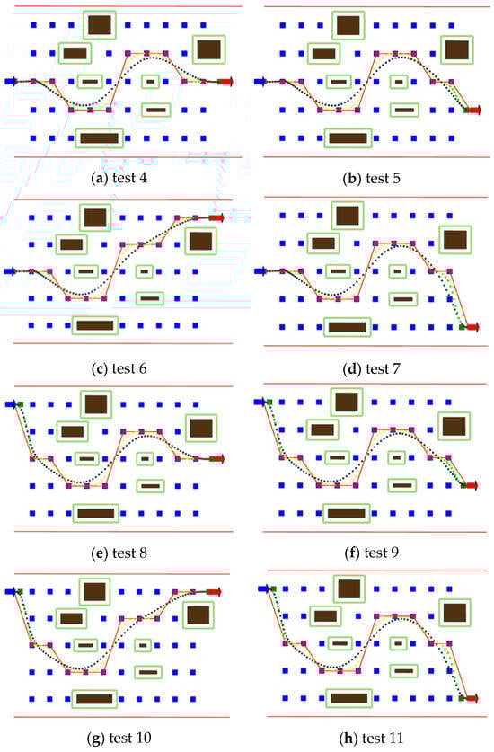
Figure 24.
Curve fitting and optimization.
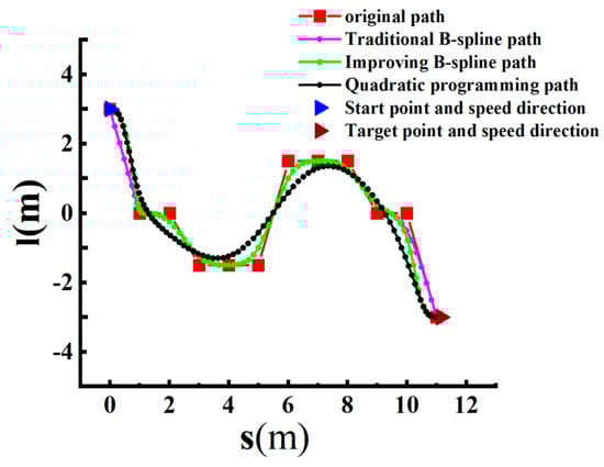
Figure 25.
Test 11 displaying the analysis in Origin.
As shown in Figure 26①, B-spline fitting eliminates the sharp corners in the original path caused by the sparse sampling points. At these corners, a smooth curve is used to ensure the smoothness of AGV motion. As depicted in Figure 26②, at both the starting and ending points, the vehicle’s velocity direction is horizontal to the right. However, traditional B-spline fitting paths do not consider velocity direction; instead, they purely fit based on the coordinates of path points. This can lead to difficulties in smoothly tracking the planned path at the starting point and pose inaccuracies at the ending point.
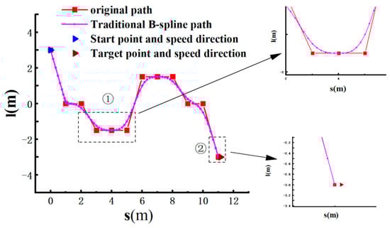
Figure 26.
Comparison before and after B-spline fitting.
As shown in Figure 27②, the improved B-spline fitting, while eliminating sharp corners, also considers the velocity direction at the starting and ending points. The green curve ultimately ensures that the vehicle reaches the endpoint with a horizontal rightward velocity. The cost values and are calculated as shown in Figure 28, and the best interpolation results are achieved when = 6 and = 7. As depicted in Figure 27①, although the improved B-spline eliminates most of the sharp corners, in areas with steeper corners, the fitted path may still not be smooth enough, and there is room for overall path improvement.
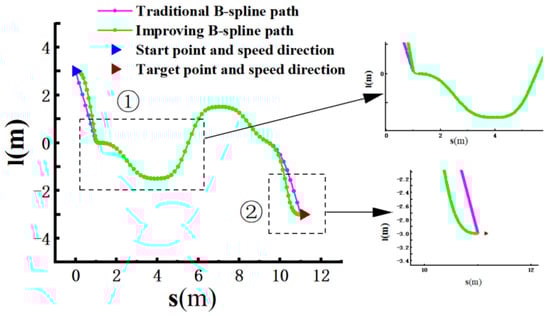
Figure 27.
Traditional B-spline and improved B-spline.
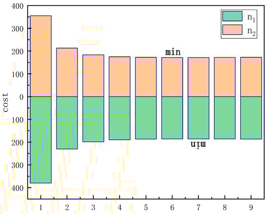
Figure 28.
Cost of .
As shown in Figure 29②, under the improved B-spline fitting path with a relatively large value for k1, the quadratic programming prioritizes smoothness. Due to the setting of segmental tolerance, it ensures that the smooth optimization does not disrupt the planned path’s velocity direction at the starting and ending points, as depicted in Figure 29① and ③.
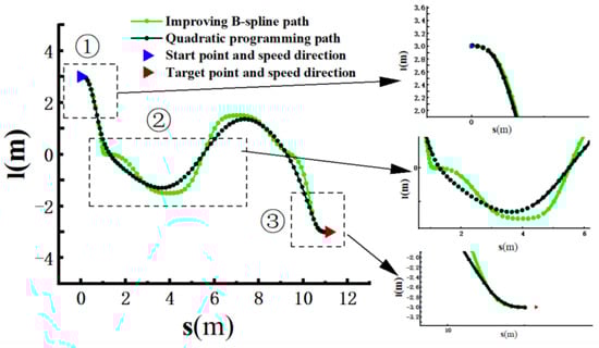
Figure 29.
Effectiveness of quadratic programming.
After a series of processing steps, the path output by quadratic programming has been fitted to create a high-quality path that aligns with the original path, ensuring smoothness, shortest-path characteristics, and proximity to the reference line. This path serves as the final result of coarse planning and is sent to precise planning. The remaining seven sets of experiments in Figure 24 all align with the conclusions drawn in the analysis above.
4.5. Validation of Lateral Planning Effectiveness in Precise Planning
As shown in Figure 30, the planning results from Section 4.4 are used as the input reference lines for precise planning, taking test6 as an example. Sampling planning is performed under the motion constraints defined in Section 3.1 to validate the planning effectiveness of the lateral planning in precise planning. The parameters used are as listed in Table 12.
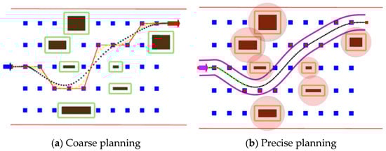
Figure 30.
Coarse planning vs. precise planning comparison.
Table 12.
Precise planning parameters.
The experimental process, as described in Section 3.2, involves calculating the optimal path using the evaluation function and then eliminating dangerous trajectories through collision detection. The vehicle is controlled to track the planned trajectory using a pure tracking algorithm. The visualization of the experimental process is shown in the following figure (Figure 31 and Figure 32) (where the pink arrow represents the AGV, and the light red circle represents the danger zone of obstacles).
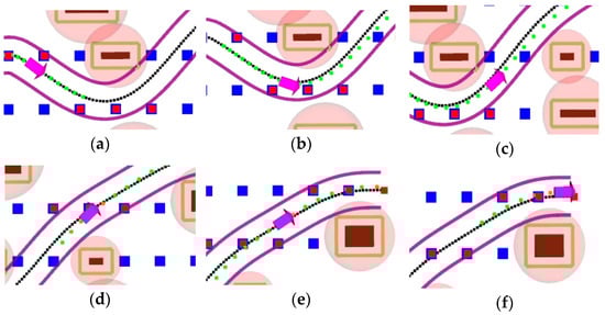
Figure 31.
Precise planning lateral planning in simulation. (a)–(f) are the precise planning experiment simulation process.
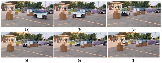
Figure 32.
Precise planning lateral planning in reality. (a)–(f) are the precise planning of the actual testing process.
Compare the reference line output by coarse planning with the planned path in precise planning as shown in Figure 33a, the planned road curvature in Figure 33b, and analyze the changes in trajectory acceleration and jerk during lateral planning as depicted in Figure 33c.
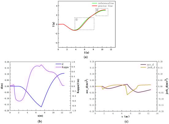
Figure 33.
Analysis of precise planning lateral planning. (a) Comparison between reference line and precise-planning trajectory. (b) Lateral acceleration and jerk. (c) Lateral deviation and planned road curvature.
Based on the experimental results, we can obtain the following conclusions.
(1) As shown in Figure 30 and Table 12, compared to coarse planning, the lateral sampling range has been reduced from [−4, 4] to [−0.5, 0.5], with lateral sampling points reduced from 80 to 10 under the condition of = 0.1. This significant reduction in the sampling range greatly improves algorithm speed while ensuring efficient, accurate, and safe lateral sampling based on the coarse planning reference line. This greatly enhances both sampling efficiency and quality.
(2) As depicted in Figure 31, although the reference line output by coarse planning is already capable of avoiding all obstacles, precise planning, due to curve fitting, optimization, and the inclusion of a safety margin (), still performs local obstacle avoidance, as shown in Figure 33a for cases ① and ②. This corresponds to (b), (e), and (f) in Figure 31. As shown in Figure 33b, the lateral deviation is between [−0.17, 0.1].
4.6. Validation of Longitudinal Planning in Precise Planning
In the experiments conducted in Section 4.4, the effectiveness of longitudinal planning in precise planning is validated by setting different initial speeds and target speeds. Four sets of speed planning experiments are conducted to evaluate its performance in small-scale acceleration and deceleration as well as large-scale acceleration and deceleration. The results of speed planning are shown in the following figure.
The experimental statistics are presented in the following table.
The experimental results indicate the following:
(1) As shown in Figure 34a–d, for small-scale acceleration and deceleration, precise planning can achieve the target speed within a single planning cycle. However, for large-scale acceleration and deceleration (0 m/s→1.5 m/s and 1.5 m/s→0.5 m/s), as observed in Figure 34f,h, it takes three and two planning cycles, respectively. This is because for significant speed changes, precise planning needs to consider factors like acceleration and jerk costs, so it cannot achieve the target speed within a single planning cycle.
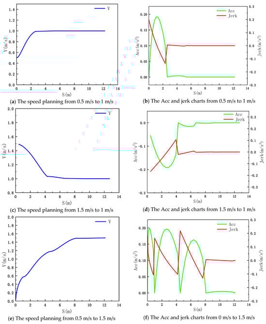
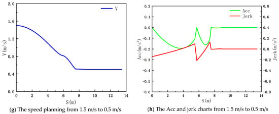
Figure 34.
Speed planning statistics chart.
(2) According to Table 13, in all four sets of experiments, the vehicles eventually reach or get close to the target speed. This indicates accurate speed planning, and the acceleration and jerk values meet the requirements in Table 12, demonstrating the effectiveness of sampling constraints based on the motion model.
Table 13.
Speed planning statistics.
(3) The maximum acceleration for all four sets of experiments reaches 0.19 m/s2, and the acceleration changes gradually under the constraints of jerk. This reflects that speed planning doesn’t blindly pursue reaching the desired speed but considers a balance between speed, longitudinal acceleration, and jerk values. This ensures the AGV’s stability while achieving the desired speed as quickly as possible.
4.7. Comparative Experiments
To validate the proposed method in this paper, it is compared with the traditional Frenet sampling planning algorithm [,,], and the experimental process is shown in the Figure 35 and Figure 36.
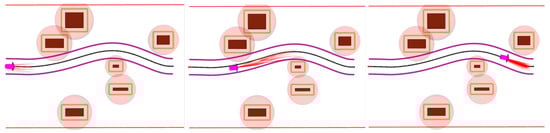
Figure 35.
Hierarchical trajectory planning algorithm.
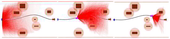
Figure 36.
Frenet sampling planning algorithm.
As described in Section 3.3, the hierarchical trajectory planning algorithm reduces the time complexity of traditional Frenet sampling planning algorithms from to . In the experiment, the hierarchical trajectory planning algorithm samples 80 sets of trajectories each time, while the traditional Frenet sampling planning algorithm samples 1156 sets of trajectories each time, Under the results of coarse planning the precise planning algorithm is applied, and the number of samples is significantly reduced. This provides an effective solution for dealing with the retrieval area of wide roads in the construction site environment.
At the same time, this paper uses the DWA planning algorithm [] to compare the hierarchical trajectory planning algorithm. The experimental process is shown in Figure 37 and Figure 38.
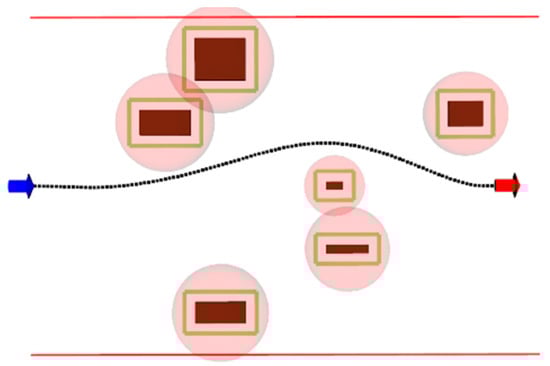
Figure 37.
Hierarchical trajectory planning algorithm compare with DWA.
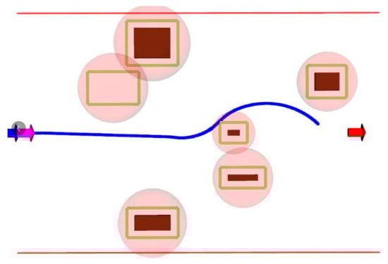
Figure 38.
DWA planning algorithm.
It can be observed that the DWA planning algorithm is a path planning algorithm that does not consider road boundaries and is used in unknown spaces. The planning results have uncertainty. The hierarchical trajectory planning algorithm can obtain a rough solution path through coarse planning, and the rough solution path is optimized through fitting, which is significantly better than the DWA planning algorithm in terms of smoothness. During the experiment, the DWA planning algorithm may also encounter the problem of local optimal traps, as shown in Figure 39. The hierarchical trajectory planning algorithm uses greedy thinking to find the optimal path from the endpoint in coarse planning, ensuring that the algorithm does not fall into local optimal traps.
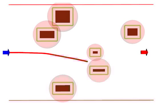
Figure 39.
DWA of local optimal trap.
Based on the experiments conducted in Section 4.3, Section 4.4, Section 4.5, Section 4.6 and Section 4.7. This paper presents a comparison table of the hierarchical trajectory planning algorithm, dynamic programming algorithm, Frenet sampling algorithm, and DWA algorithm as follows: According to Table 14, although dynamic programming algorithms have high efficiency and no local traps, it cannot smooth paths and does not have speed planning. The disadvantage of Frenet sampling planning is that it frequently solves solutions of fifth and fourth polynomials over a wide range of horizontal and lateral directions, resulting in low running efficiency. DWA planning may fall into local traps, and the RRT algorithm does not have the ability to optimize speed planning and curve smoothing. Through comparison with various algorithms, it was found that the hierarchical trajectory planning algorithm is a trajectory planning algorithm with high operational efficiency, no local traps, smooth trajectory optimization, and has the capable of speed planning. In the table, × represents that the corresponding function has defects, while √ represents that it has the corresponding function.
Table 14.
Algorithm comparison.
5. Conclusions
This paper constructs a hierarchical trajectory planning algorithm through the design of two algorithms: coarse planning based on road environment sampling and precise planning based on AGV motion sampling. The hierarchical trajectory planning algorithm ensures efficient algorithm operation while also considering the smoothness of the planned trajectory. It ensures that high-capacity AGVs can output accurate, safe, and smooth planned paths efficiently and stably on wide retrieval roads in a construction site environment.
In the final tests and experiments, we conducted tests based on AGV real vehicles in a real construction site environment. From the actual test results, the dynamic programming algorithm for coarse planning can quickly select the optimal path. The interpolated B-spline fitting method, considering the nonholonomic constraints of the vehicle, ensures the rationality of the path while eliminating the planning turning points. Secondary optimization further ensures the smoothness of the path. Fine planning, based on coarse planning, reduces the lateral sampling range from 8 m to 1 m. In the speed planning process, various acceleration and deceleration scenarios of AGV were tested. The experimental results show that the planned trajectory meets collision detection requirements while achieving the desired speed rapidly and considering trajectory smoothness. In all test experiments, the maximum acceleration was 0.1944 m/s2, and the maximum jerk was 0.1972 m/s3, indicating good speed planning performance. This implementation achieves high-quality and efficient trajectory planning.
This research effectively addresses challenges faced by AGVs in construction site environments, such as heavy loads, wide road sampling ranges, and random obstacle distributions. It provides new insights into solving path planning problems in construction site environments. The proposed hierarchical trajectory planning algorithm can be used for single AGV working conditions. It can be further improved while considering the cooperation of multiple vehicles. In the future, we are planning to integrate the leader follower control, game theory and other algorithms for planning and control under multi vehicle working conditions to meet the real requirements of building sites.
Author Contributions
Conceptualization, Y.B., P.L. and W.L.; Methodology, Y.B. and W.L.; Software, Y.B.; Validation, Y.B.; Formal analysis, W.L.; Resources, Z.C. and P.Y.; Writing—original draft, Y.B. All authors have read and agreed to the published version of the manuscript.
Funding
This research was funded by the National Natural Science Foundation of China under Grant 52175007, the China Postdoctoral Science Foundation under Grant 2018M630348/2019T120259, and the Yangtze River Delta HIT robot technology research institute under Grant HIT-CXY-CMP2-ADTIL-21-01.
Data Availability Statement
Data are contained within the article.
Conflicts of Interest
The authors declare that they have no known competing financial interests or personal relationships that could have appeared to influence the work reported in this paper.
References
- Ge, X.; Li, L.; Chen, H. Research on Online Scheduling Method for Flexible Assembly Workshop of Multi-AGV System Based on Assembly Island Mode. In Proceedings of the 2021 IEEE 7th International Conference on Cloud Computing and Intelligent Systems (CCIS), Xi’an, China, 7–8 November 2021; pp. 371–375. [Google Scholar] [CrossRef]
- Lian, Y.; Zhang, L.; Xie, W.; Wang, K. An Improved Heuristic Path Planning Algorithm for Minimizing Energy Consumption in Distributed Multi-AGV Systems. In Proceedings of the 2020 International Symposium on Autonomous Systems (ISAS), Guangzhou, China, 6–8 December 2020; pp. 70–75. [Google Scholar] [CrossRef]
- Yang, J.; Yu, F.; Wu, E.; Yang, Y. Energy saving of automated terminals considering AGV speed variation. In Proceedings of the 2022 International Symposium on Sensing and Instrumentation in 5G and IoT Era (ISSI), Shanghai, China, 17–18 November 2022; pp. 68–73. [Google Scholar] [CrossRef]
- Macias-Sola, J.; Uttendorf, S.; Blech, J.O. A Ground Texture-based Mapping and Localization Method for AGVs. In Proceedings of the 2021 International Conference on Indoor Positioning and Indoor Navigation (IPIN), Lloret de Mar, Spain, 29 November–2 December 2021; pp. 1–6. [Google Scholar] [CrossRef]
- Zhu, H.; Liu, J. Improved Harmony Search Algorithm and Application in Optimal Scheduling of Hospital Transport AGV. In Proceedings of the 2021 IEEE International Conference on Electrical Engineering and Mechatronics Technology (ICEEMT), Qingdao, China, 2–4 July 2021; pp. 739–743. [Google Scholar] [CrossRef]
- Wang, H.; Chen, T.; Wang, S.; Lu, B. Semantic Segmentation Algorithms for Ground AGV and UAV Medical Transport Scenes. In Proceedings of the 2022 16th ICME International Conference on Complex Medical Engineering (CME), Zhongshan, China, 4–6 November 2022; pp. 252–255. [Google Scholar] [CrossRef]
- Jodejko-Pietruczuk, A.; Werbińska-Wojciechowska, S. Availability assessment for a multi-AGV system based on simulation modeling approach. In Proceedings of the 2021 International Conference on Electrical, Computer, Communications and Mechatronics Engineering (ICECCME), Mauritius, Mauritius, 7–8 October 2021; pp. 1–6. [Google Scholar] [CrossRef]
- Spišáková, M.; Mésáros, P.; Kaleja, P.; Mandičák, T. Virtual Reality as a Tool for Increasing Safety of Construction Sites. In Proceedings of the 2020 18th International Conference on Emerging eLearning Technologies and Applications (ICETA), Košice, Slovenia, 12–13 November 2020; pp. 1–6. [Google Scholar] [CrossRef]
- Wu, H.-T.; Yu, W.-D.; Gao, R.-J.; Wang, K.-C.; Liu, K.-C. Measuring the Effectiveness of VR Technique for Safety Training of Hazardous Construction Site Scenarios. In Proceedings of the 2020 IEEE 2nd International Conference on Architecture, Construction, Environment and Hydraulics (ICACEH), Hsinchu, Taiwan, 25–27 December 2020; pp. 36–39. [Google Scholar] [CrossRef]
- Wang, C.; Mao, J. Summary of AGV Path Planning. In Proceedings of the 2019 3rd International Conference on Electronic Information Technology and Computer Engineering (EITCE), Xiamen, China, 18–20 October 2019; pp. 332–335. [Google Scholar] [CrossRef]
- Yuan, H.; Zhang, G.; Li, Y.; Liu, K.; Yu, J. Research and implementation of intelligent vehicle path planning based on four-layer neural network. In Proceedings of the 2019 Chinese Automation Congress (CAC), Hangzhou, China, 22–24 November 2019; pp. 578–582. [Google Scholar] [CrossRef]
- Zu, W.; Fan, G.; Gao, Y.; Ma, Y.; Zhang, H.; Zeng, H. Multi-UAVs Cooperative Path Planning Method based on Improved RRT Algorithm. In Proceedings of the 2018 IEEE International Conference on Mechatronics and Automation (ICMA), Changchun, China, 5–8 August 2018; pp. 1563–1567. [Google Scholar] [CrossRef]
- Liu, Q.; Cheng, X.; Hui, J.; Ming, R. Research on Robot Path Planning Method Based on Tangent Intersection Method. In Proceedings of the 2020 International Conference on Information Science, Parallel and Distributed Systems (ISPDS), Xi’an, China, 14–16 August 2020; pp. 272–276. [Google Scholar] [CrossRef]
- Shi, K.; Wu, P.; Liu, M. Research on path planning method of forging handling robot based on combined strategy. In Proceedings of the 2021 IEEE International Conference on Power Electronics, Computer Applications (ICPECA), Shenyang, China, 22–24 January 2021; pp. 292–295. [Google Scholar] [CrossRef]
- Zhu, J.; Zhao, S.; Zhao, R. Path Planning for Autonomous Underwater Vehicle Based on Artificial Potential Field and Modified RRT. In Proceedings of the 2021 International Conference on Computer, Control and Robotics (ICCCR), Shanghai, China, 8–10 January 2021; pp. 21–25. [Google Scholar] [CrossRef]
- Jin, Y. Research on Path Planning of Airport VIP Service Robot Based on A* Algorithm and Artificial Potential Field Method. In Proceedings of the 2021 5th Asian Conference on Artificial Intelligence Technology (ACAIT), Haikou, China, 29–31 October 2021; pp. 485–489. [Google Scholar] [CrossRef]
- Yao, J. Path Planning Algorithm of Indoor Mobile Robot Based on ROS System. In Proceedings of the 2023 IEEE International Conference on Image Processing and Computer Applications (ICIPCA), Changchun, China, 28–30 June 2023; pp. 523–529. [Google Scholar] [CrossRef]
- Ma, B.; Wei, C.; Huang, Q.; Hu, J. APF-RRT*: An Efficient Sampling-Based Path Planning Method with the Guidance of Artificial Potential Field. In Proceedings of the 2023 9th International Conference on Mechatronics and Robotics Engineering (ICMRE), Shenzhen, China, 10–12 February 2023; pp. 207–213. [Google Scholar] [CrossRef]
- Bi, Q.; Pian, J.; Wu, F.; Dai, Y. Research on Robot Path Planning Based on Improved Genetic Algorithm. In Proceedings of the 2022 China Automation Congress (CAC), Xiamen, China, 25–27 November 2022; pp. 242–246. [Google Scholar] [CrossRef]
- Chen, Z.; Gao, Q.; Wang, X.; Liu, X. Local path planning of intelligent vehicle based on improved artificial potential field. In Proceedings of the 2020 IEEE 3rd International Conference on Electronic Information and Communication Technology (ICEICT), Shenzhen, China, 13–15 November 2020; pp. 110–116. [Google Scholar] [CrossRef]
- Li, J.; Zhang, J. Global path planning of unmanned boat based on improved ant colony algorithm. In Proceedings of the 2021 4th International Conference on Electron Device and Mechanical Engineering (ICEDME), Guangzhou, China, 19–21 March 2021; pp. 176–179. [Google Scholar] [CrossRef]
- Fan, W.; Li, Y.; Yang, J.; Wang, B. Global path planning method for mobile vehicles based on Goal-Optimized JPS algorithm. In Proceedings of the 2023 26th International Conference on Electrical Machines and Systems (ICEMS), Zhuhai, China, 5–8 November 2023; pp. 2498–2501. [Google Scholar] [CrossRef]
- Peng, Q.; Guo, H.; Hu, C. Graph Embedding and Approximate Dynamic Programming for the Reliable Shortest Path Problem. In Proceedings of the 2021 IEEE International Intelligent Transportation Systems Conference (ITSC), Indianapolis, IN, USA, 19–22 September 2021; pp. 653–659. [Google Scholar] [CrossRef]
- Barros, R.M.; Lage, G.G.; De Andrade Lira Rabêlo, R. Graph Shortest Path and Dynamic Programming Applied to Sequencing ORD Control Adjustments. In Proceedings of the 2023 IEEE Belgrade PowerTech, Belgrade, Serbia, 25–29 June 2023; pp. 1–6. [Google Scholar] [CrossRef]
- Jiang, S.; Zhang, Y.; Liu, R.; Jafari, M.; Kharbeche, M. Data-Driven Optimization for Dynamic Shortest Path Problem Considering Traffic Safety. IEEE Trans. Intell. Transp. Syst. 2022, 23, 18237–18252. [Google Scholar] [CrossRef]
- Ren, J.; Huang, X. Dynamic Programming Inspired Global Optimal Path Planning for Mobile Robots. In Proceedings of the 2021 IEEE 4th International Conference on Information Systems and Computer Aided Education (ICISCAE), Dalian, China, 24–26 September 2021; pp. 461–465. [Google Scholar] [CrossRef]
- Gamayanti, N.; Kadir, R.E.A.; Alkaff, A. Global Path Planning for USV Waypoint Guidance System Using Dynamic Programming. In Proceedings of the 2020 International Seminar on Intelligent Technology and Its Applications (ISITIA), Surabaya, Indonesia, 22–23 July 2020; pp. 248–253. [Google Scholar] [CrossRef]
- Kusuma, Z.D.S.; Indriawati, K.; Widjiantoro, B.L.; Hija, A.I.; Nurhadi, H. Optimal Trajectory Planning Generation for Autonomous Vehicle Using Frenet Reference Path. In Proceedings of the 2022 5th International Seminar on Research of Information Technology and Intelligent Systems (ISRITI), Yogyakarta, Indonesia, 8–9 December 2022; pp. 480–484. [Google Scholar] [CrossRef]
- Zhang, D.; Zhao, J.; Jiao, X. Trajectory planning of autonomous vehicle based on Frenét frame system. In Proceedings of the 2021 China Automation Congress (CAC), Beijing, China, 22–24 October 2021; pp. 7973–7977. [Google Scholar] [CrossRef]
- Teng, Q.; Wang, X.; Han, B.; Liu, J.; Tang, M. Research on the trajectory planning method of inland waterway vessels based on Frenet coordinate system. In Proceedings of the 2023 7th International Conference on Transportation Information and Safety (ICTIS), Xi’an, China, 4–6 August 2023; pp. 644–650. [Google Scholar] [CrossRef]
- Wang, X.; Yu, H.; Liu, J. Research on Local Path Planning Algorithm Based on Frenet Coordinate System. In Proceedings of the 2022 4th International Conference on Machine Learning, Big Data and Business Intelligence (MLBDBI), Shanghai, China, 28–30 October 2022; pp. 249–252. [Google Scholar] [CrossRef]
- Lin, X.; Cao, N.; Lin, Y. Optimal control for a class of nonlinear systems with state delay based on Adaptive Dynamic Programming with ε-error bound. In Proceedings of the 2013 IEEE Symposium on Adaptive Dynamic Programming and Reinforcement Learning (ADPRL), Singapore, 16–19 April 2013; pp. 177–182. [Google Scholar] [CrossRef]
- Zhang, Y.; Xiao, Z.; Yuan, X.; Li, S.; Liang, S. Obstacle Avoidance of Two-Wheeled Mobile Robot based on DWA Algorithm. In Proceedings of the 2019 Chinese Automation Congress (CAC), Hangzhou, China, 22–24 November 2019; pp. 5701–5706. [Google Scholar] [CrossRef]
- Yang, H.; Li, H.; Liu, K.; Yu, W.; Li, X. Research on path planning based on improved RRT-Connect algorithm. In Proceedings of the 2021 33rd Chinese Control and Decision Conference (CCDC), Kunming, China, 22–24 May 2021; pp. 5707–5712. [Google Scholar] [CrossRef]
Disclaimer/Publisher’s Note: The statements, opinions and data contained in all publications are solely those of the individual author(s) and contributor(s) and not of MDPI and/or the editor(s). MDPI and/or the editor(s) disclaim responsibility for any injury to people or property resulting from any ideas, methods, instructions or products referred to in the content. |
© 2024 by the authors. Licensee MDPI, Basel, Switzerland. This article is an open access article distributed under the terms and conditions of the Creative Commons Attribution (CC BY) license (https://creativecommons.org/licenses/by/4.0/).