Fast and Accurate Short-Term Load Forecasting with a Hybrid Model

Abstract

Short-term electric load forecasting (STLF) plays a pivotal role in modern power system management, bolstering forecasting accuracy and efficiency. This enhancement assists power utilities in formulating robust operational strategies, consequently fostering economic and social advantages within the systems. Existing methods employed for STLF either exhibit poor forecasting performance or require longer computational time. To address these challenges, this paper introduces a hybrid learning approach comprising variational mode decomposition (VMD) and random vector functional link network (RVFL). The RVFL network, serving as a universal approximator, showcases remarkable accuracy and fast computation, owing to the randomly generated weights connecting input and hidden layers. Additionally, the direct links between hidden and output layers, combined with the availability of a closed-form solution for parameter computation, further contribute to its efficiency. The effectiveness of the proposed VMD-RVFL was assessed using electric load datasets obtained from the Australian Energy Market Operator (AEMO). Moreover, the effectiveness of the proposed method is demonstrated by comparing it with existing benchmark forecasting methods using two performance indices such as root mean square error (RMSE) and mean absolute percentage error (MAPE). As a result, our proposed method requires less computational time and yielded accurate and robust prediction performance when compared with existing methods.

1. Introduction

Effective electricity power supply planning is a pivotal aspect of modern power system management. Accurate forecasting holds significant advantages for tasks such as unit commitment, power system security, and energy transfer scheduling [1,2,3,4]. According to [5], even a modest 1% reduction in forecast error can result in substantial cost savings for a utility with a 1 GW peak, approximately 300,000 dollars per year for short-term electric load forecasting [5]. As a result, the primary goal of load forecasting is to secure a reliable power supply while concurrently minimizing operational costs and reducing energy wastage.

Electric load forecasting falls within the domain of time series forecasting and can be classified into three categories based on the forecasting horizon: short term (minutes to one day ahead), medium term (weeks to months ahead), and long term (years ahead) [6]. This study predominantly focuses on short-term load forecasting [7], specifically forecasting load for the next day. The complexity of electric load forecasting arises from diverse exogenous factors, including special occasions, weather conditions, economic fluctuations, etc., leading to highly non-linear and intricate patterns in load data [8].

Since the 1940s, various statistical-based linear time series forecasting methods, such as Holt–Winters exponential smoothing [9], autoregressive integrated moving average (ARIMA) [10], and linear regression [11], have been pivotal in projecting future energy requirements. These statistical learning models now commonly serve as the foundation for contemporary electric load forecasting research [12]. Fan and Hyndman [13] proposed a short-term load forecasting model with non-linear relationships and serially correlated errors in a regression framework.

Artificial Neural Networks (ANNs), a popular machine learning technique with universal approximation capabilities, have been widely used in diverse fields, including control, biomedical, manufacturing, and power system management [14]. Hong [11] extensively studied short-term load forecasting using ANNs, regression analysis, and fuzzy regression models. Among these, ANNs have shown tremendous success in time series forecasting [15]. The commonly used training method for ANNs is the back-propagation (BP) supervised learning algorithm [5], which, however, has drawbacks such as slow convergence and susceptibility to local minimum trapping [16].

The random vector functional link (RVFL) network, as introduced by Pao et al. [17], stands out as a randomized neural network architecture. It enhances training efficiency through random weight assignment and direct links between input and output layers [18,19,20]. Notably, the hidden layer’s random weights and biases remain fixed throughout the learning process [15,21]. The output layer weights are computed using a non-iterative closed-form solution [22,23]. This approach enables RVFL to mitigate the shortcomings associated with BP-based neural networks, such as susceptibility to local optima, slow convergence, and sensitivity to learning rates [15,22,24,25,26,27,28]. An independently developed method, the single hidden layer neural network with random weights (RWSLFN), was reported in [29], differing from RVFL by excluding the direct links. Research has shown that the direct links significantly enhances RVFL’s performance, especially in time series forecasting [27,30,31,32,33]. In [16,31,33], the authors clearly demonstrated that the presence of the direct links in RVFL help to regularize the randomization and reduce the model complexity.

Ensemble learning, or hybrid methods, improve forecasting by combining multiple algorithms strategically. The advantages lie in statistical, computational, and representational aspects [34]. Ensemble methods can be parallel or sequential [35]. In parallel methods, the training signal is decomposed into sub-datasets, individually analyzed, and then combined to formulate final output. Sequential methods use outputs from one model as inputs for another method. Examples of parallel methods include wavelet decomposition [36], empirical mode decomposition (EMD) [37], and variational mode decomposition (VMD) [38].

The VMD method decomposes a time series input into an ensemble of band-limited intrinsic mode functions (IMFs) within the frequency domain [38]. For each of the decomposed IMFs, their center frequencies and corresponding bandwidths are concurrently and nonrecursively estimated within the Hilbert space. Moreover, through iterative updates of the IMFs in the Fourier domain, VMD achieves minimal reconstruction error, resembling a filter tuned with a predetermined center frequency [38]. This makes VMD robust against mode-mixing defects and additive noise components compared to EMD and its variants. Several ensemble methods based on EMD have been proposed across various research domains [39,40]. For instance, in [39], EMD and its enhanced variants are integrated with Support Vector Regression (SVR) and ANNs to tackle challenges in wind speed forecasting. Consistent experimental results indicate that EMD-based models tend to outperform their individual learning counterparts. Similarly, EMD-RVFL, as highlighted in [40], demonstrates superior performance compared to RVFL and other EMD-based approaches. However, the EMD method decomposes electric load time series based on time–domain characteristics, facing performance challenges due to mode-mixing. This occurs when IMFs of EMD share similar frequency bands or when each IMF contains a wide range of frequencies. Moreover, EMD variants such as Ensemble EMD (EEMD) and Complete EEMD with Adaptive Noise (CEEMDAN) encounter challenges related to high computational complexity, primarily stemming from the significant number of shifting iterations required during the signal decomposition process. Additionally, these approaches are susceptible to the deteriorative impact of additive noise when reconstructing time series from the IMFs. While many existing hybrid methods utilize the mentioned statistical techniques for forecasting these IMFs, it has been observed that certain predominant IMFs exhibit significant non-stationary and non-linear characteristics. These issues adversely affect the forecasting performance of hybrid methods [39,41].

To overcome the abovementioned issues, we employed the VMD to decompose the electric load into IMFs, so that the non-linear and non-stationary behavior of the electric load can be reduced. To predict and model each IMF, we employed RVFL due to its notable performance in fast and accurate prediction. The hybrid method employed for electric load prediction, referred to as VMD-RVFL [42], was assessed using electric load datasets acquired from the Australian Energy Market Operator (AEMO) [43]. Comparative analysis involved evaluating VMD-RVFL against state-of-the-art methods such as VMD-RVM [44], VMD-SVR [45], and VMD-ELM [46]. Forecasting efficacy was assessed using two performance metrics: root mean square error (RMSE) and mean absolute percentage error (MAPE). The findings underscored that the proposed VMD-RVFL method outperformed existing approaches in accurately forecasting electric load and took less computation time. While the individual algorithms VMD and RVFL are well-established, their integration into the VMD-RVFL structure [42] is a novel approach that has not been previously explored for STLF. To the best of our knowledge, our implementation of VMD-RVFL represents the pioneering exploration of this combined methodology for STLF. VMD provides precise decomposition, complemented by the RVFL network’s ability to deliver accurate and fast predictions.

The rest of this paper is organized as follows. In Section 2, the brief description of VMD, RVFL, and the VMD-RVFL employed for electric load forecasting are discussed. Section 3 discusses the datasets and performance indices for performance evaluation. Later, results and discussion are provided in Section 4. Finally, Section 5 concludes the paper.

2. Materials and Methods

In this section, we will provide a brief overview of existing techniques, encompassing variational mode decomposition (VMD) and random vector functional link (RVFL). Following this, we will delve into the proposed VMD-RVFL specifically designed for electric load forecasting.

2.1. Variational Mode Decomposition (VMD) Process

As a decomposition technique, the VMD proposed by the authors of [38] is highly effective for transforming a non-stationary time series into a stationary form by identifying a set of decomposed components called intrinsic mode functions (IMFs). In this analysis, the electric load series $p\left(t\right)$ is transformed into different IMFs with a sparsity property, generating a new and simpler stationary series. Each extracted IMF ($m_j$) from the original load series is assumed to be predominantly centered around a frequency called the central frequency ($w_j$), a parameter ascertained during the decomposition process. The principle of decomposition is fundamentally based on the following points:

1.

Application of the Hilbert transform calculates the associated signal of each IMF $m_j$ to derive a unilateral frequency spectrum.

2.

Shifting each spectrum of $m_j$ to the baseband is accomplished by mixing it with an exponential function tuned to the respective computed central frequency.

3.

Determination of the bandwidth of $m_j$ is based on the H1 Gaussian smoothness of the shifted signal.

The formulation of VMD when considered as a problem with constraints is presented in Equation (1):

$$\underset{m_j,w_j}{min}\left\{\sum _{j=1}^J{∥{\delta }_t\left[(\delta \left(t\right)+\frac{k}{\pi t})*m_j\left(t\right)\right]e^{-k{w}_{j}t}∥}^2\right\}$$

(1)

$$\sum _{j=1}^J{m}_j=p\left(t\right)$$

(2)

Here, $p\left(t\right)$ represents the original series, J is the number of IMF, ‘*’ denotes convolution, and the set of all IMFs is denoted as $\left\{m_j\right\}=\{m_1,m_2,m_3,m_4,\dots ,m_J\}$ with the corresponding central frequencies: $\left\{w_j\right\}=\{w_1,w_2,w_3,w_4,\dots ,w_J\}$. Additionally, $\delta \left(t\right)$ represents the Dirac delta function with a time horizon ‘t’, and k is the complex square root of −1.

Equation (1) is reformulated as Equation (3), incorporating a quadratic penalty term and introducing a Lagrange multiplier ($\lambda$), effectively addressing an optimization problem devoid of constraints:

$$\begin{array}{cc}\hfill L(m_j,w_j,\lambda )=& \alpha \left\{\sum _{j=1}^J{∥{\delta }_t\left[(\delta \left(t\right)+\frac{k}{\pi t})*m_j\left(t\right)\right]e^{-k{w}_{j}t}∥}^2\right\}\hfill \\ \hfill & +\alpha \left\{{∥p\left(t\right)-\sum _{j=1}^J{m}_j∥}^2\langle \lambda \left(t\right),p\left(t\right)-\sum _{j=1}^J{m}_j\left(t\right)\rangle \right\}\hfill \end{array}$$

(3)

VMD utilizes the Alternating Direction Method of Multipliers (ADMMs) to acquire distinct components known as IMFs and determine the central frequency of each IMF during the shifting process. By employing the ADMMs method, the optimization problem described in Equation (1) can be effectively solved, yielding the resulting $m_j$ and $w_j$ as detailed below:

$${\widehat{m}}_j^{n+1}=\frac{\widehat{y}\left(w\right)-{\sum }_{i\ne j}{\widehat{m}}_i\left(w\right)+\widehat{\lambda }\left(w\right)/2}{1+2\alpha {(w-w_k)}^2}$$

(4)

$${\widehat{w}}_{n+1}^j=\frac{{\int }_0^{\infty }w{\left|{\widehat{m}}_j\left(w\right)\right|}^{2}dw}{{\int }_0^{\infty }{\left|m_j\left(w\right)\right|}^{2}dw}$$

(5)

where n is the number of iterations; $\widehat{y}\left(w\right)$, ${\widehat{m}}_i\left(w\right)$, $\widehat{\lambda }\left(w\right)$, and ${\widehat{m}}_{n+1}^j$ are the Fourier transform of $p\left(t\right)$, $m_j\left(t\right)$, $\lambda \left(t\right)$, and $m_{n+1}^j$, respectively.

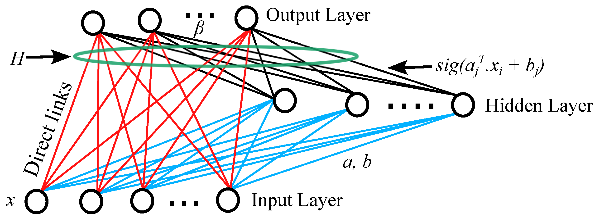
2.2. Random Vector Functional Link (RVFL)

The RVFL network [18] constitutes a single-layer feed-forward neural network that distinguishes itself by the absence of iterative training, such as back-propagation (BP). Conversely, it incorporates the direct links from the input layer to the output layer as depicted in Figure 1 (with red color). The inputs are associated with randomly assigned weights, linking them to the hidden neurons within the hidden layer. In the RVFL architecture, the direct link to the output node does not necessitate the assignment of any weights.

In the context of prediction analysis, the output layer consists of a single node responsible for delivering the predicted sample derived from RVFL processing. To gauge the prediction accuracy of the proposed model, errors are determined. Notably, since the weights between the hidden layer (hidden layer neurons) and the input layer are randomly selected, only the output weights need to be calculated. The operational procedure of the RVFL is elucidated below.

Suppose that we have a dataset $\left\{(x_i,y_i)\right|x_i\in {\mathbb{R}}^v,y_i\in {\mathbb{R}}^u,$ i = 1,2,3, …, N}. An RVFL network is defined as

$$f_i=\sum _{j=1}^P{\beta }_{j}h\left(a_j^{T}x+b_j\right)+\sum _{j=P+1}^{P+L}{\beta }_j{x}_j$$

(6)

where P is the number of hidden layer neurons ($j=1,2,\dots ,P$); $h(·)$ represents the activation function; x denotes the input ($x=[x_1,x_2,\dots ,x_L]$); $a_i$ signifies the weight between the input and hidden layer neuron; $b_i$ stands for the bias for the hidden layer; $a_i·x+b_i$ expresses the weighted input with bias; L indicates the number of inputs; and ${\beta }_j$ denotes the connection between the hidden neuron and the output neuron. The input neurons are also directly connected to the output node, and the number of direct connections is denoted as L, where L ranges from $P+1$ to $P+L$. Here, the sigmoid, or sig, is utilized as an activation function in RVFL processing and is defined as

$$f_i=\sum _{j=1}^P{\beta }_{j}sig\left(a_j^T.x_i+b_j\right)+\sum _{j=P+1}^{P+L}{\beta }_j{x}_j,i=1,2,\dots ,N$$

(7)

where

$$\beta ={\left[\begin{array}{c}{\beta }_1\\ ⋮\\ {\beta }_{P+L}\end{array}\right]}_{(P+L)\times 1}$$

(8)

$\beta$ represents the output weights.

$$R={\left[\begin{array}{c}{t}_1\\ ⋮\\ t_N\end{array}\right]}_{N\times 1}$$

(9)

R shows real output.

The whole right-hand side of Equation (7) can be represented by H. This H can be expanded as below:

$$H={\left[\begin{array}{cccc}sig(a_1,b_1,x_1)& \dots & sig(a_P,b_P,x_1)& x_1\\ ⋮& \ddots & ⋮& ⋮\\ sig(a_1,b_1,x_N)& \dots & sig(a_P,b_P,x_N)& x_N\end{array}\right]}_{N\times (P+L)}$$

(10)

Here, H represents the concatenation of the hidden layer output features and input nodes via direct links. As earlier explained, the input node directly connected to the output node via direct link does not require assigning any weights as depicted in Figure 1 [30,33,42]. The addition of these direct links in RVFL serves to regularize the model, resulting in improved generalization performance and lower model complexity.

Hence, the matrix expression for the RVFLN equation can be further represented as

$$R=H\beta$$

(11)

The calculation is carried out directly using the Moore–Penrose pseudoinverse matrix formulation.

Thus, directly from Equation (11), we calculate $\beta$ as given below:

$$\beta ={\left(H^{T}H\right)}^{-1}{H}^{T}R=H^{+}R$$

(12)

where $H^{+}={\left(H^{T}H\right)}^{-1}{H}^T$ and + shows the Moore–Penrose pseudoinverse.

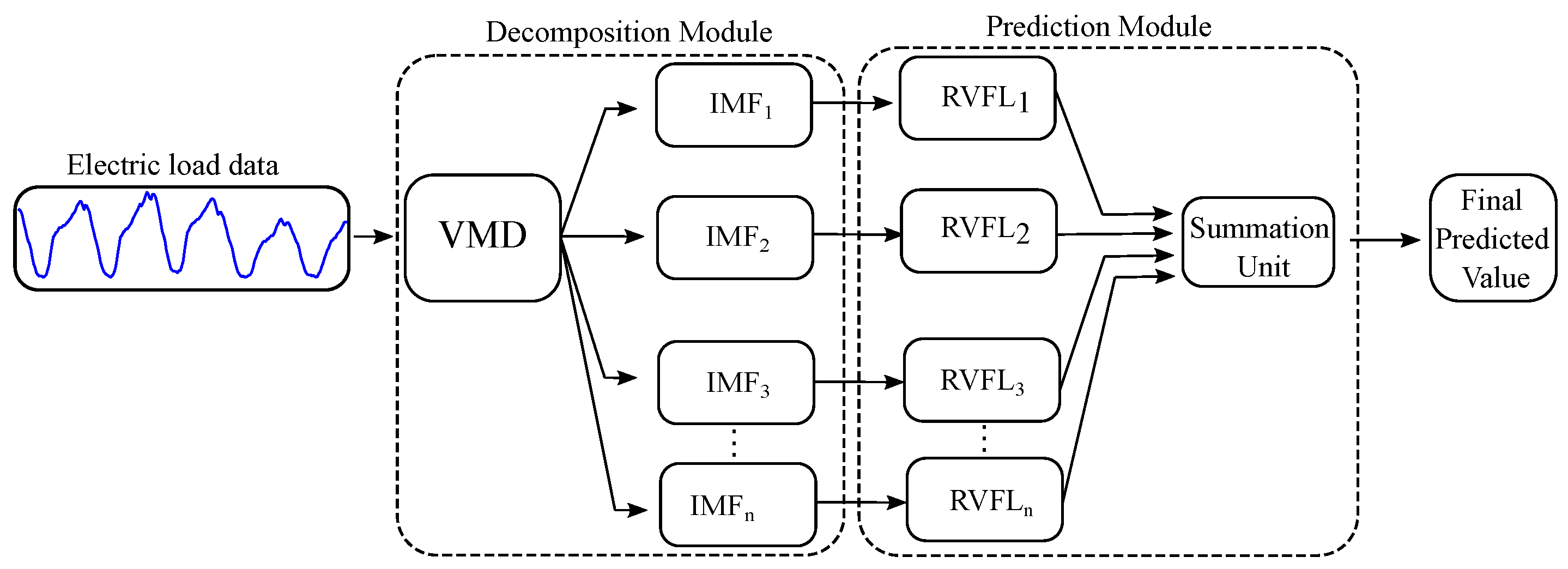
2.3. Electric Load Forecasting with VMD-RVFL

In this study, we utilize an ensemble approach referred to as the “divide and conquer” method. This technique involves breaking down the original time series into a sequence of sub-datasets until they attain a level of simplicity conducive to analysis. For the VMD-RVFL network, as shown in Figure 2, the electricity load demand data are subjected to decomposition into multiple intrinsic mode functions (IMFs) using the VMD method. Subsequently, a separate RVFL network is trained for each IMF. The ultimate prediction results are obtained by aggregating the outputs from all sub-series through straightforward summation. In this way, VMD-RVFL structure addresses all the issues related to inaccurate forecasting of electric load. This implies that VMD reduces the non-linear and non-stationary behavior of the electric load by decomposing it into various IMFs, which are accurately modeled by the fast and accurate RVFL predictor. The overall procedures can be summarized as follows:

1.

In the initial phase, we employ VMD to break down respiratory motion into IMFs ($IM{F}_1$, $IM{F}_2$, $IM{F}_3$,…, $IM{F}_n$) and a residual component (R), as illustrated in the decomposition module of Figure 2. This process focuses on tackling the intra-trace variabilities and irregularities inherent in respiratory motion through decomposition strategies.

2.

Secondly, we construct a training dataset ${\mathbf{X}}_t$ to serve as the input for each RVFL network ($RVF{L}_1$, $RVF{L}_2$,…, $RVF{L}_n$, $RVF{L}_r$) corresponding to each extracted IMF and residue. ${\mathbf{X}}_t$ is defined as a sequence of inputs: $\mathbf{X}t=[x_1,x_2,\dots ,x_t,x_{t+1},\dots ]$, where $x_t$ represents the magnitude of respiratory motion recorded at time instant t. Predicting respiratory motion for a known horizon $\tau$ can be approached as a classical learning problem, aiming to estimate the relationship between elements in the input space ${\mathbf{X}}_t\in {\mathbb{R}}^m$ and elements in the target space $y\in \mathbb{R}$. The elements in the input space are formulated by considering the recent history of the respiratory motion trace: $\mathbf{X}t=[x_t,x_{t-1},\dots ,x_{t-m}]$, with m representing the dimension of the input feature vector. The elements in the target space corresponding to ${\mathbf{X}}_t$ are defined as $y_t=x_{t+\tau }$. Here, ${\widehat{x}}_{t+\tau }$ denotes the predicted value $\tau$ samples ahead, computed at the tth sample.

3.

Subsequently, input vectors along with their corresponding target vectors, formulated using the training data from $IM{F}_1$, $IM{F}_2$, $IM{F}_3$,…, $IM{F}_n$ are fed into the $RVF{L}_1$, $RVF{L}_2$, $RVF{L}_3$,…, $RVF{L}_n$ models. These models learn a non-linear mapping that captures the intrinsic relationship between the input feature space and the target space. This phase is depicted in the prediction module of Figure 2.

4.

During this phase, the non-linear mapping established during the training stages of $RVF{L}_1$, $RVF{L}_2$, $RVF{L}_3$,…, $RVF{L}_n$ will be applied to predict unseen data for all $IM{F}_1$, $IM{F}_2$, $IM{F}_3$,…, $IM{F}_n$.

5.

Lastly, sum up the predicted outputs of all RVFL networks ($RVF{L}_1$, $RVF{L}_2$, $RVF{L}_3$,…, $RVF{L}_n$) to formulate the predicted output ${\widehat{x}}_{t+\tau }$ as illustrated in the summation unit of Figure 2.

3. Experimental Setup

In this section, we will discuss the datasets and their statistical properties. Subsequently, we will provide detailed explanations of the two performance measures used to evaluate the prediction performance of the model.

3.1. Datasets

In this study, we utilized electric load datasets sourced from the Australian Energy Market Operator (AEMO) [43] to assess the effectiveness of benchmark learning models. The dataset comprises a total of fifteen electric load datasets spanning the years 2013 to 2015, representing five Australian states: New South Wales (NSW), Tasmania (TAS), Queensland (QLD), South Australia (SA), and Victoria (VIC). The training phase involved the initial nine months of each dataset, with the subsequent three months reserved for testing. A summary of the dataset statistics is provided in

Table 1. Summary of AEMO load datasets.

Dataset	Year	Length	Min	Median	Mean	Max	Std
QLD	2013	17,520	4148.7	5752.1	5703.7	8278.4	747.0
	2014	17,520	4073.0	5726.0	5745.7	8445.3	794.0
	2015	17,520	4281.4	6005.6	6035.4	8808.7	777.2
NSW	2013	17,520	5113.0	8045.0	7981.6	13,788	1190.9
	2014	17,520	5138.1	7987.4	7917.8	11,846	1170.1
	2015	17,520	5337.4	7990.4	7979.8	12,602	1232.7
TAS	2013	17,520	659.5	1109.0	1129.3	1650.3	142.3
	2014	17,520	569.1	1088.7	1109.7	1630.1	139.0
	2015	17,520	479.4	1112.3	1138.2	1667.2	145.3
SA	2013	17,520	728.6	1389.3	1426.6	2991.3	301.7
	2014	17,520	682.5	1360.8	1403.3	3245.9	312.8
	2015	17,520	696.3	1352.7	1398.5	2870.4	306.0
VIC	2013	17,520	3551.6	5458.1	5511.8	9587.5	895.9
	2014	17,520	3272.9	5307.8	5324.4	10240	921.4
	2015	17,520	3369.1	5186.5	5194.6	8579.9	864.7

.

The electric load data are sampled every half an hour, resulting in the recording of 48 data points per day. To discern cycles and patterns within the load time series (TS), we utilize the autocorrelation function (ACF) to guide the selection of an informative feature subset. Let X be a time series dataset given as $X=\{X_t:t\in T\}$, where T represents the index set. The autocorrelation coefficient $r_k$ at lag k can be computed as follows:

$$r_k=r(X_t,X_{t-k})=\frac{{\sum }_{t=k+1}^n(X_t-\overline{X})(X_{t-k}-\overline{X})}{{\sum }_{t=1}^n{(X_t-\overline{X})}^2}$$

(13)

where $\overline{X}$ represents the mean value of all observations in the given time series, and $r_k$ quantifies the linear correlation between the time series at times t and $t-k$.

To measure the strength and direction of the relationship between two variables, we have employed the autocorrelation function (ACF). In the context of time series analysis, correlation coefficients help us understand the degree of linear association between a variable at different time points. From the ACF plot in Figure 3, illustrating the ACF for electricity load data within a one-week time window, we can discern the presence of three prominent lag variables with significant dependencies. These variables include the value recorded in the previous half-hour ($X_{t-1}$), the value at the same time one week ago ($X_{t-336}$), and the value at the same time one day prior ($X_{t-48}$). In order to encompass all pertinent lag variables, we incorporate data points spanning the entire previous day ($X_{t-48}$ to $X_{t-96}$) and the corresponding day from the preceding week ($X_{t-336}$ to $X_{t-384}$) to construct the input feature set for one-day-ahead load forecasting in our study. Based on this setting, we provided this input to the proposed VMD-RVFL network for accurate forecasting.

After the VMD, we obtain $m\times n$ IMFs and m residues. Let us denote the IMFs and residues as $X_{i,j}$, where $1\le i\le m$ and $1\le j\le n+1$. For each IMF and residue, when predicting the value at time t (denoted as $X_{i,j,t}$), the corresponding input features consist of the data points from the entire previous day ($X_{i,j,t-48}$ to $X_{i,j,t-96}$) and the same day in the previous week ($X_{i,j,t-336}$ to $X_{i,j,t-384}$).

This forms the content of the input matrix for the RVFL analyzing the sub-series. Consequently, the predicted values for all the sub-series at time t are given by

$$\{{\widehat{X}}_{i,j,t}:1\le i\le m,1\le j\le n+1\}$$

(14)

For the time series load datasets, all the training and testing values are linearly scaled to [0, 1]. The scaling is performed separately and independently for each year using the following formula:

$${\overline{y}}_i=\frac{y_{\max }-y_i}{y_{\max }-y_{\min }}$$

(15)

where $y_i$ represents the value of the ith point in the dataset, ${\overline{y}}_i$ is the corresponding scaled value, and $y_{\max }$ and $y_{\min }$ are the maximum and minimum values of the dataset, respectively.

3.2. Performance Indices

Two error measures are employed to assess the performance of learning models in this study: root mean square error (RMSE) and mean absolute percentage Eerror (MAPE), defined as follows:

$$\mathrm{RMSE}=\sqrt{\frac{1}{n}\sum _{i=1}^n{(y_i-{\widehat{y}}_i)}^2}$$

(16)

$$\mathrm{MAPE}=\frac{1}{n}\sum _{i=1}^n\left|\frac{y_i-{\widehat{y}}_i}{y_i}\right|$$

(17)

where ${\widehat{y}}_i$ is the predicted value corresponding to $y_i$, and n is the number of data points in the testing time series (TS) dataset. The hybrid approach employed for electric load prediction is denoted as VMD-RVFL [42]. The effectiveness of the VMD-RVFL was evaluated using electric load datasets obtained from the Australian Energy Market Operator (AEMO). The VMD-RVFL was compared to state-of-the-art VMD-RVM [44], VMD-SVR [45], and VMD-ELM [46]. The results obtained with these two performance indices demonstrate that the proposed VMD-RVFL outperforms existing forecasting methods in accurate forecasting of electric load.

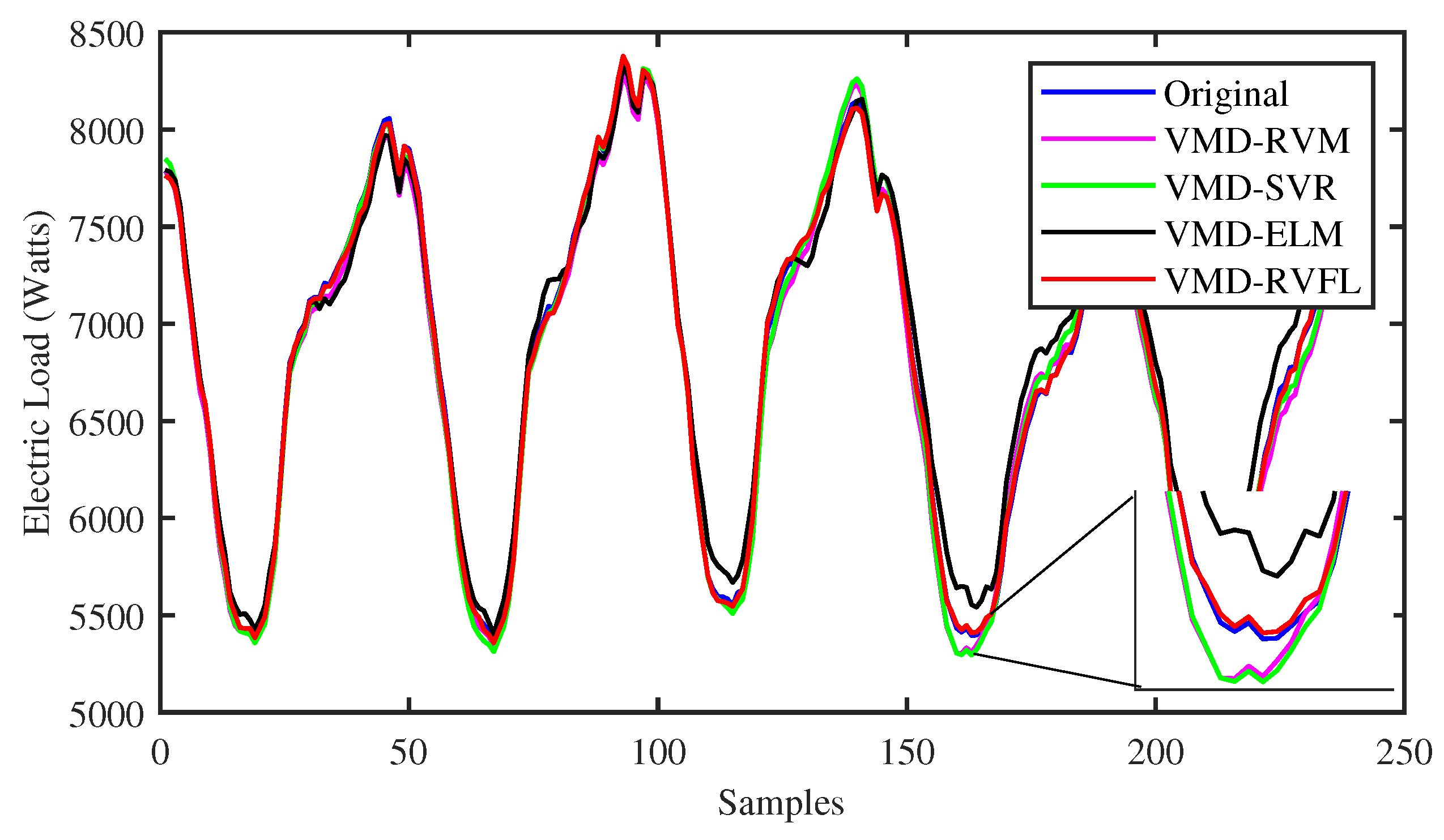
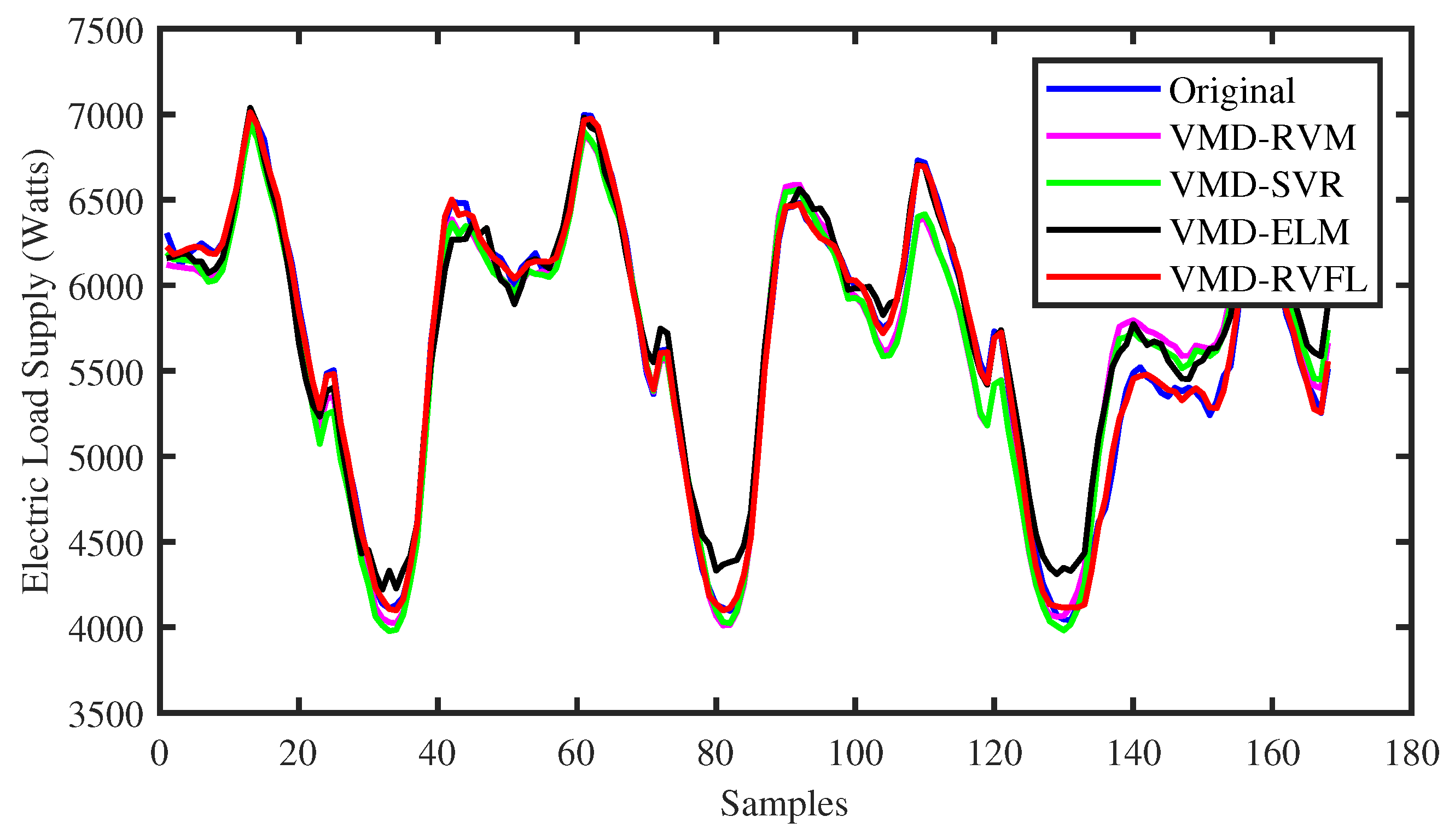
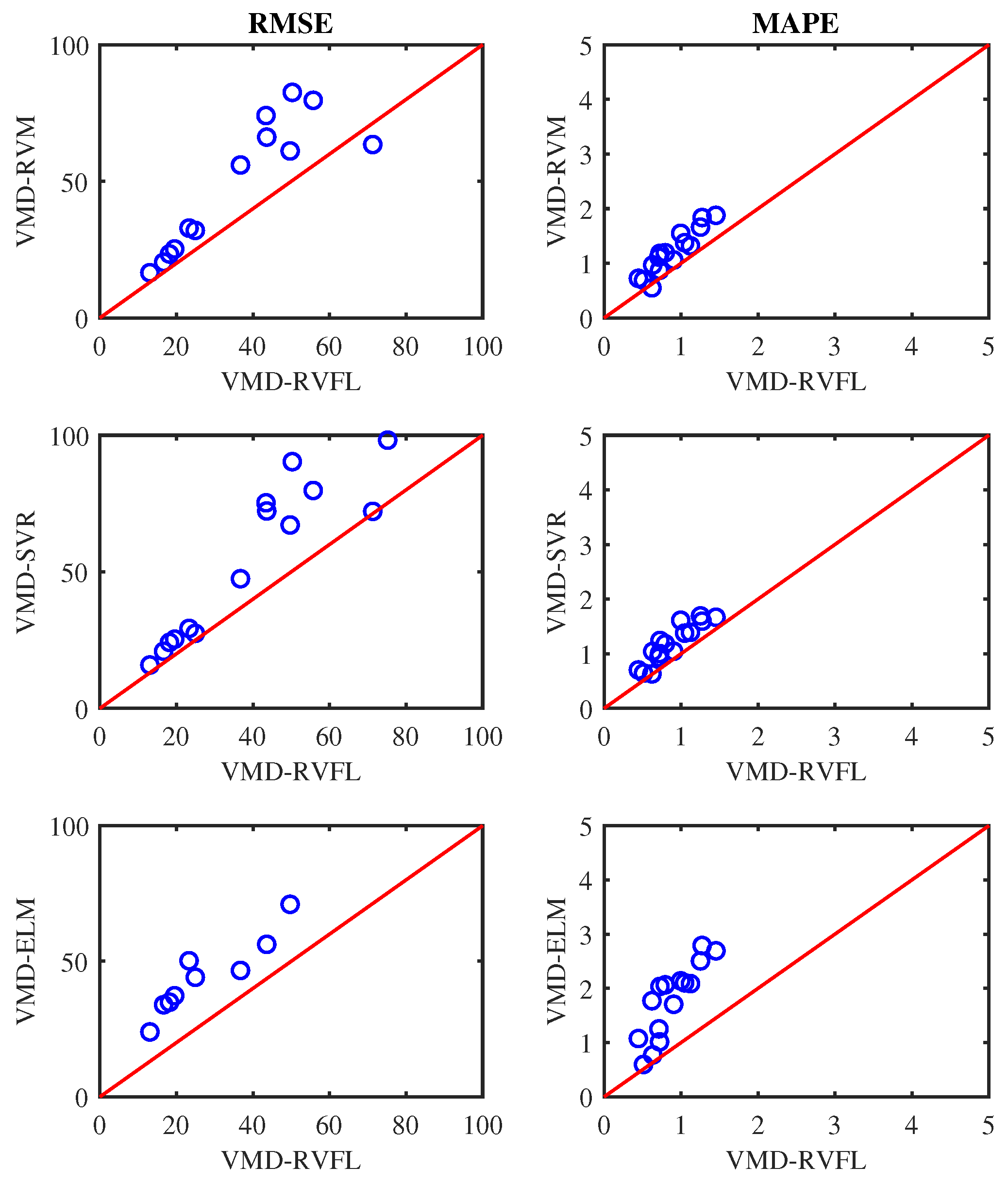
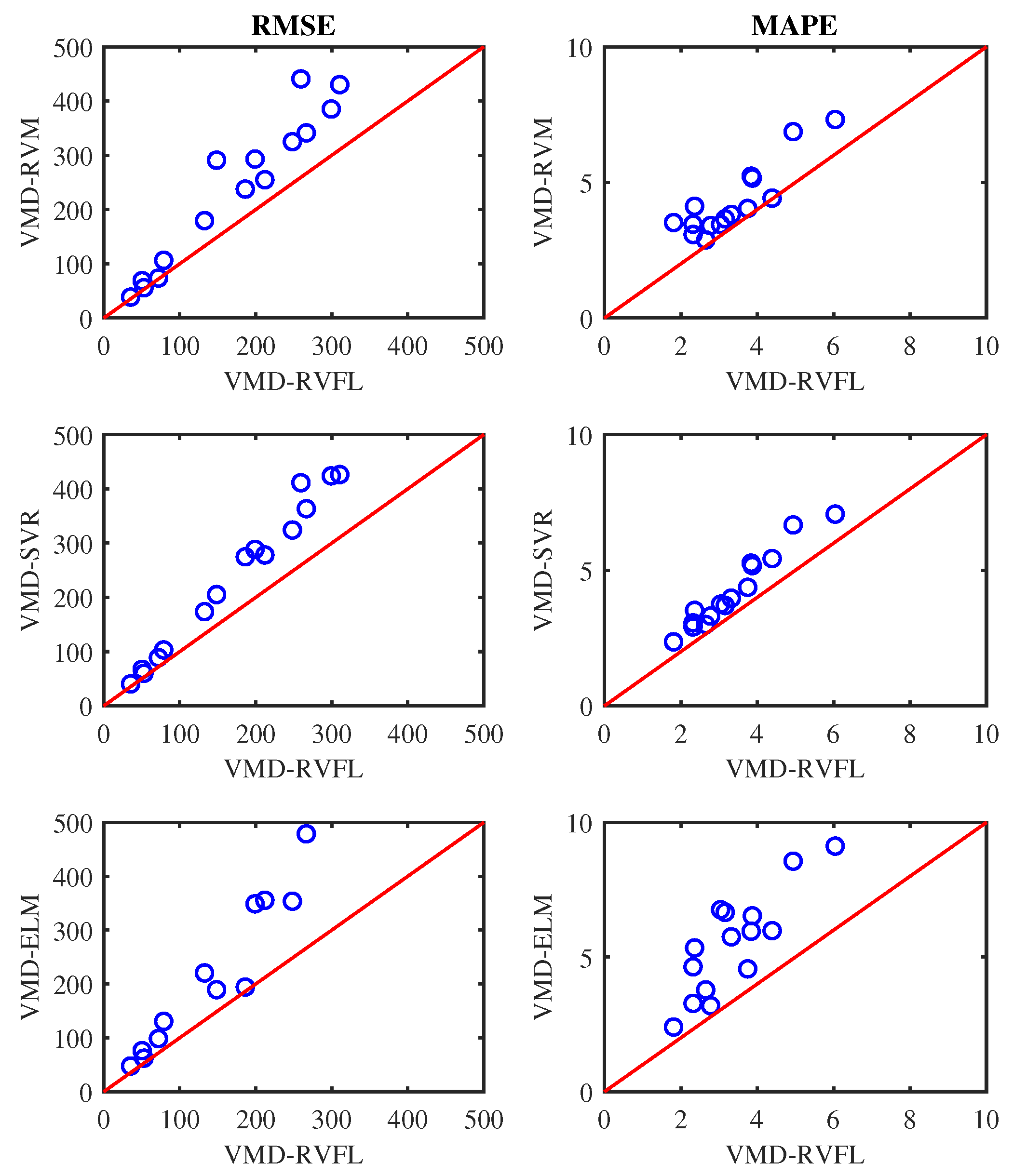
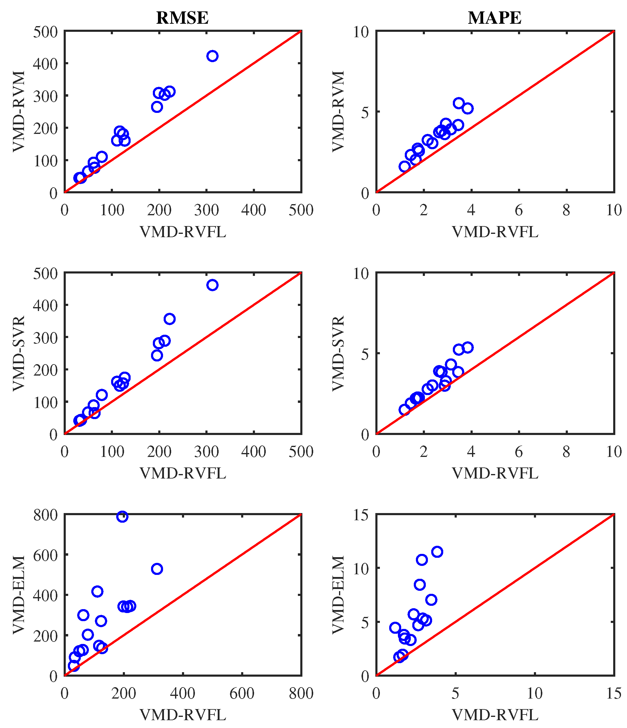
4. Results and Discussion

In this section, we assess the performance of the VMD-RVFL approach by comparing it with several benchmark methods. We have selected 15 IMFs for VMD operation in each learning model. The example for the VMD on electric load is presented in Figure 4. It is evident from our analysis that VMD serves as an effective tool in mitigating the non-linear characteristics inherent in electric load data. By increasing the number of IMFs, we observe a gradual reduction in the non-linear behavior exhibited by the electric load, as demonstrated in detail in Figure 4. This reduction in non-linearity in the electric load in the form of IMFs with VMD will help the predictor to predict the future value accurately [42]. Initially, the performance of learning models in this study is compared using the persistence method, the most basic forecasting technique. Because the electric load time series is very periodic, the persistence approach uses the load value at the same hour of the previous day as the prediction for each of the 24 h of the next day. This technique works well. The parameters of all the methods were optimized. The results for half day and one-day-ahead electric load forecasting predictions are presented in

Table 2. Statistical comparison for half-day-ahead load forecasting in terms of RMSE.

Dataset	Year	Metrics	Persistence	VMD-RVM	VMD-SVR	VMD-ELM	VMD-RVFL
QLD	2013	RMSE	292.58	61.12	67.13	70.99	49.69
	2014	RMSE	270.70	66.19	72.26	56.23	43.58
	2015	RMSE	240.04	55.98	47.47	46.61	36.72
NSW	2013	RMSE	470.05	115.21	98.18	137.85	75.18
	2014	RMSE	348.01	74.08	75.26	108.04	43.39
	2015	RMSE	505.88	63.45	72.11	181.14	71.24
TAS	2013	RMSE	60.58	20.35	20.89	33.78	16.66
	2014	RMSE	32.58	25.23	25.33	37.21	19.66
	2015	RMSE	29.80	16.53	15.87	23.98	13.02
SA	2013	RMSE	145.88	32.88	29.21	50.54	23.23
	2014	RMSE	165.33	23.36	24.19	34.95	18.51
	2015	RMSE	128.99	32.09	27.27	44.04	24.92
VIC	2013	RMSE	320.55	82.53	90.37	141.44	50.17
	2014	RMSE	325.10	116.62	117.89	146.28	71.88
	2015	RMSE	320.55	79.62	79.78	148.69	55.75

,

Table 3. Statistical comparison for half-day-ahead load forecasting in terms of MAPE (%).

Dataset	Year	Metrics	Persistence	VMD-RVM	VMD-SVR	VMD-ELM	VMD-RVFL
QLD	2013	MAPE	3.78	0.87	1.00	1.01	0.72
	2014	MAPE	3.15	0.96	1.04	0.77	0.63
	2015	MAPE	2.8	0.69	0.64	0.59	0.51
NSW	2013	MAPE	3.18	0.72	0.78	1.07	0.44
	2014	MAPE	3.58	1.11	0.93	1.24	0.71
	2015	MAPE	3.98	0.55	0.63	1.77	0.62
TAS	2013	MAPE	2.99	1.31	1.39	2.08	1.11
	2014	MAPE	3.45	1.66	1.69	2.50	1.25
	2015	MAPE	3.5	1.04	1.04	1.70	0.90
SA	2013	MAPE	7.89	1.83	1.59	2.79	1.27
	2014	MAPE	7.25	1.37	1.37	2.10	1.04
	2015	MAPE	8.87	1.87	1.66	2.69	1.45
VIC	2013	MAPE	6.45	1.54	1.61	2.13	0.99
	2014	MAPE	5.14	1.18	1.24	2.03	0.75
	2015	MAPE	5.12	1.19	1.18	2.06	0.79

,

Table 4. Statistical comparison for one-day-ahead load forecasting in terms of RMSE.

Dataset	Year	Metrics	Persistence	VMD-RVM	VMD-SVR	VMD-ELM	VMD-RVFL
QLD	2013	RMSE	492.58	291.02	205.07	189.36	148.48
	2014	RMSE	588.70	341.37	363.39	478.79	266.49
	2015	RMSE	453.07	293.16	288.50	348.78	199.02
NSW	2013	RMSE	901.51	325.09	324.14	353.69	248.21
	2014	RMSE	878.07	385.28	423.94	662.85	299.32
	2015	RMSE	1055.406	440.84	411.32	532.81	259.41
TAS	2013	RMSE	97.85	38.67	40.46	47.69	35.37
	2014	RMSE	86.86	68.94	67.35	76.12	50.49
	2015	RMSE	83.99	55.77	60.09	62.18	52.87
SA	2013	RMSE	288.77	179.54	173.62	220.52	132.59
	2014	RMSE	242.23	73.71	88.79	98.61	71.95
	2015	RMSE	265.14	106.40	103.15	130.51	78.89
VIC	2013	RMSE	781.68	430.24	426.36	523.44	310.49
	2014	RMSE	719.40	237.72	274.77	194.27	186.17
	2015	RMSE	874.69	254.98	278.19	355.49	211.98

and

Table 5. Statistical comparison for one-day-ahead load forecasting in terms of MAPE (%).

Dataset	Year	Metrics	Persistence	VMD-RVM	VMD-SVR	VMD-ELM	VMD-RVFL
	2013	MAPE	6.38	3.52	2.36	2.40	1.81
	2014	MAPE	7.14	3.66	3.70	6.66	3.16
	2015	MAPE	6.63	3.46	3.06	4.64	2.32
NSW	2013	MAPE	8.65	3.08	2.91	3.28	2.33
	2014	MAPE	8.51	3.45	3.75	6.76	3.04
	2015	MAPE	9.68	4.12	3.52	5.34	2.36
TAS	2013	MAPE	6.87	2.88	3.00	3.78	2.65
	2014	MAPE	6.51	5.23	5.26	5.96	3.84
	2015	MAPE	6.03	4.04	4.37	4.56	3.75
SA	2013	MAPE	16.02	7.32	7.07	9.12	6.04
	2014	MAPE	14.41	4.42	5.43	5.98	4.39
	2015	MAPE	15.39	6.87	6.67	8.56	4.94
VIC	2013	MAPE	10.71	5.16	5.17	6.53	3.87
	2014	MAPE	11.24	3.41	3.31	3.19	2.78
	2015	MAPE	10.86	3.82	3.97	5.75	3.32

. Values in bold indicate that the respective method attains the highest performance for this dataset according to the specified performance measurement. Table 2 and Table 4 indicate that the proposed VMD-RVFL method consistently demonstrates superior performance in the case of RMSE. We have observed the same performance in the case of MAPE as illustrated in Table 3 and Table 5.

To identify the specific forecast intervals where the proposed VMD-RVFL method excels in performance, a comparison was made between the forecasting results of the VMD-RVFL and the other methods. Figure 5 and Figure 6 illustrate the comparisons of predicted values with actual values for the proposed method and other networks for half day ahead. In addition, Figure 7, Figure 8 and Figure 9 demonstrate the predictive capabilities for complete one-day-ahead forecasting. This analysis focuses on a selected portion of the load data from the testing dataset of QLD for the year 2015, covering a time window of one week (from Sunday to Saturday). The datasets used in all five of these figures correspond to five different months of the year 2015. As analyzed, the prediction performance by the proposed method for half day and one day ahead is more accurate as compared to other methods. The prediction performance of all methods is more erroneous in case of one day ahead compared to half day ahead due to the large forecasting horizon. The main reason behind the successful performance of VMD-RVFL is the presence of the direct links, which help to regularize the randomization process, leading to better generalization performance.

Figure 10, Figure 11 and Figure 12 display scatter plots illustrating the averaged RMSE and MAPE achieved by all methods for half, one, and one-and-a-half-day-ahead forecasting. In these figures, if a circle marker falls above the diagonal line, it signifies that VMD-RVFL outperforms other methods. Conversely, if a circle marker is below the diagonal line, it indicates superior performance of other methods over VMD-RVFL. Based on this analysis, it can be concluded that VMD-RVFL outperformed other methods in terms of both indices for most of the datasets. The improved prediction accuracy observed in VMD-RVFL underscores the successful integration of the enhanced learning capabilities of RVFL with VMD.

Additionally, statistical tests were employed to conduct a comprehensive analysis of the performance disparities among all the hybrid models. Friedman’s test was utilized to assess the null hypothesis that the effects across columns are equal against the alternative hypothesis that they are not. Friedman’s ANOVA, conducted at a significance level of 0.01, revealed p-values of $8.922\times {10}^{-18}$ and $1.729\times {10}^{-7}$ for MAPE and RMSE, respectively. Following this, the results of the subsequent post hoc analysis, which employed Bonferroni correction, are presented in Figure 13a,b. This in-depth analysis highlighted significant differences in the average performance of VMD-RVFL compared to other methods concerning both MAPE and RMSE, as depicted in Figure 13a and Figure 13b, respectively.

We conducted comparative simulations across distinct seasons using the 2015 load dataset from NSW, selecting January, April, July, and October to capture the unique seasonal factors in each geographical area. The performance of all models was assessed across these seasons, and the outcomes are presented in

Table 6. Predictive outcomes for various seasons based on the load data from NSW in the year 2015.

Month	Metrics	Persistence	VMD-RVM	VMD-SVR	VMD-ELM	VMD-RVFL
Jan	RMSE	842.732	256.151	296.022	424.44	167.135
	MAPE	7.393	2.810	3.0102	4.9952	1.766
Apr	RMSE	769.606	128.519	141.163	525.474	97.955
	MAPE	6.801	1.252	1.359	5.674	0.956
Jul	RMSE	989.372	389.809	360.240	645.186	233.994
	MAPE	9.831	3.857	3.480	6.369	2.176
Oct	RMSE	1620.508	302.301	248.087	244.602	96.339
	MAPE	14.887	2.891	2.188	2.384	0.998

Note: MAPE values are in %.

. Upon analysis, taking into account the diverse factors present in different seasons, we observed a relative stability in the performance of benchmark methods when applied to the same dataset. Moreover, amidst these varying conditions, the VMD-RVFL method consistently exhibited superior performance compared to all benchmark models.

Figure 14 illustrates the computational time required by benchmark methods for electric load forecasting using datasets from the year 2013. The analysis was performed on a PC equipped with an Intel Core i7-6700 CPU operating at 3.40 GHz and 16 GB of RAM, utilizing MATLAB R2023a. To ensure a fair comparison, an equal number of training and testing data samples were employed in all methods to determine the computational time for one-day-ahead forecasting. Benefiting from the closed-form solution of RVFL and ELM, the VMD-RVFL and VMD-ELM models demonstrate fast computation speeds compared to other methods. Specifically, VMD-RVFL exhibits faster performance than VMD-ELM due to the inclusion of direct links in VMD-RVFL. Conversely, SVR and RVM utilize iterative learning methods, grid search techniques, and a trial-and-error approach for parameter tuning. Consequently, VMD-RVM and VMD-SVR experience prolonged execution times and sensitivity to parameter adjustments.

5. Conclusions

As a solution to counter the issues of the non-linearity and non-stationary nature present in electric load, we employed the VMD-RVFL hybrid approach for accurate and fast electric load forecasting. The performance of the VMD-RVFL is evaluated using fifteen electric load datasets from AEMO, and comparisons are made with several benchmark methods. Two performance measures were employed to verify the effectiveness of the models. Based on the simulation experiments, VMD-RVFL outperformed the existing methods in the accurate forecasting of electric load. Since VMD requires a large amount of computational time for decomposition, our future work will focus on employing the elastic version of VMD (eVMD) to reduce computational time. Additionally, we will evaluate this eVMD unit with RVFL (eVMD-RVFL) for fast and accurate STLF by comparing it with state-of-the-art methods.

References

1. Alfares, H.K.; Nazeeruddin, M. Electric load forecasting: Literature survey and classification of methods. Int. J. Syst. Sci. 2002, 33, 23–34. [Google Scholar] [CrossRef]
2. Xiao, L.; Shao, W.; Yu, M.; Ma, J.; Jin, C. Research and application of a combined model based on multi-objective optimization for electrical load forecasting. Energy 2017, 119, 1057–1074. [Google Scholar] [CrossRef]
3. Lusis, P.; Khalilpour, K.R.; Andrew, L.; Liebman, A. Short-term residential load forecasting: Impact of calendar effects and forecast granularity. Appl. Energy 2017, 205, 654–669. [Google Scholar] [CrossRef]
4. Chahkoutahi, F.; Khashei, M. A seasonal direct optimal hybrid model of computational intelligence and soft computing techniques for electricity load forecasting. Energy 2017, 140, 988–1004. [Google Scholar] [CrossRef]
5. Qiu, X.; Suganthan, P.N.; Amaratunga, G.A. Ensemble incremental learning random vector functional link network for short-term electric load forecasting. Knowl.-Based Syst. 2018, 145, 182–196. [Google Scholar] [CrossRef]
6. Koprinska, I.; Rana, M.; Agelidis, V.G. Correlation and instance based feature selection for electricity load forecasting. Knowl.-Based Syst. 2015, 82, 29–40. [Google Scholar] [CrossRef]
7. Zhang, J.; Wei, Y.M.; Li, D.; Tan, Z.; Zhou, J. Short term electricity load forecasting using a hybrid model. Energy 2018, 158, 774–781. [Google Scholar] [CrossRef]
8. Zhang, M.G. Short-term load forecasting based on support vector machines regression. In Proceedings of the 2005 International Conference on Machine Learning and Cybernetics, Guangzhou, China, 18–21 August 2005; Volume 7, pp. 4310–4314. [Google Scholar]
9. Taylor, J.W. Short-term electricity demand forecasting using double seasonal exponential smoothing. J. Oper. Res. Soc. 2003, 54, 799–805. [Google Scholar] [CrossRef]
10. Lee, C.M.; Ko, C.N. Short-term load forecasting using lifting scheme and ARIMA models. Expert Syst. Appl. 2011, 38, 5902–5911. [Google Scholar] [CrossRef]
11. Hong, T. Short Term Electric Load Forecasting. Ph.D. Thesis, Faculty of North Carolina State University, Raleigh, NC, USA, 2010. [Google Scholar]
12. Goude, Y.; Nedellec, R.; Kong, N. Local short and middle term electricity load forecasting with semi-parametric additive models. IEEE Trans. Smart Grid 2013, 5, 440–446. [Google Scholar] [CrossRef]
13. Fan, S.; Hyndman, R.J. Short-term load forecasting based on a semi-parametric additive model. IEEE Trans. Power Syst. 2011, 27, 134–141. [Google Scholar] [CrossRef]
14. Leshno, M.; Lin, V.Y.; Pinkus, A.; Schocken, S. Multilayer feedforward networks with a nonpolynomial activation function can approximate any function. Neural Netw. 1993, 6, 861–867. [Google Scholar] [CrossRef]
15. Gao, R.; Du, L.; Yuen, K.F.; Suganthan, P.N. Walk-forward empirical wavelet random vector functional link for time series forecasting. Appl. Soft Comput. 2021, 108, 107450. [Google Scholar] [CrossRef]
16. Zhang, G.; Patuwo, B.E.; Hu, M.Y. Forecasting with artificial neural networks: The state of the art. Int. J. Forecast. 1998, 14, 35–62. [Google Scholar] [CrossRef]
17. Pao, Y.H.; Phillips, S.M.; Sobajic, D.J. Neural-net computing and the intelligent control of systems. Int. J. Control 1992, 56, 263–289. [Google Scholar] [CrossRef]
18. Pao, Y.H.; Park, G.H.; Sobajic, D.J. Learning and generalization characteristics of the random vector functional-link net. Neurocomputing 1994, 6, 163–180. [Google Scholar] [CrossRef]
19. Ganaie, M.; Tanveer, M.; Malik, A.K.; Suganthan, P. Minimum variance embedded random vector functional link network with privileged information. In Proceedings of the 2022 International Joint Conference on Neural Networks (IJCNN), Padua, Italy, 18–23 July 2022; pp. 1–8. [Google Scholar]
20. Malik, A.K.; Ganaie, M.; Tanveer, M.; Suganthan, P.N. Extended features based random vector functional link network for classification problem. IEEE Trans. Comput. Soc. Syst. 2022, 1–10. [Google Scholar] [CrossRef]
21. Malik, A.K.; Tanveer, M. Graph embedded ensemble deep randomized network for diagnosis of Alzheimer’s disease. IEEE ACM Trans. Comput. Biol. Bioinform. 2022, 1–13. [Google Scholar] [CrossRef]
22. Ganaie, M.; Sajid, M.; Malik, A.; Tanveer, M. Graph Embedded Intuitionistic Fuzzy RVFL for Class Imbalance Learning. arXiv 2023, arXiv:2307.07881. [Google Scholar]
23. Sharma, R.; Goel, T.; Tanveer, M.; Suganthan, P.; Razzak, I.; Murugan, R. Conv-ERVFL: Convolutional Neural Network Based Ensemble RVFL Classifier for Alzheimer’s Disease Diagnosis. IEEE J. Biomed. Health Inform. 2022, 27, 4995–5003. [Google Scholar] [CrossRef]
24. Suganthan, P.N. On non-iterative learning algorithms with closed-form solution. Appl. Soft Comput. 2018, 70, 1078–1082. [Google Scholar] [CrossRef]
25. Malik, A.K.; Gao, R.; Ganaie, M.; Tanveer, M.; Suganthan, P.N. Random vector functional link network: Recent developments, applications, and future directions. Appl. Soft Comput. 2023, 143, 110377. [Google Scholar] [CrossRef]
26. Shi, Q.; Katuwal, R.; Suganthan, P.N.; Tanveer, M. Random vector functional link neural network based ensemble deep learning. Pattern Recognit. 2021, 117, 107978. [Google Scholar] [CrossRef]
27. Gao, R.; Li, R.; Hu, M.; Suganthan, P.N.; Yuen, K.F. Significant wave height forecasting using hybrid ensemble deep randomized networks with neurons pruning. Eng. Appl. Artif. Intell. 2023, 117, 105535. [Google Scholar] [CrossRef]
28. Ahmad, N.; Ganaie, M.A.; Malik, A.K.; Lai, K.T.; Tanveer, M. Minimum variance embedded intuitionistic fuzzy weighted random vector functional link network. In Proceedings of the International Conference on Neural Information Processing, New Delhi, India, 22–26 November 2022; Springer: Berlin/Heidelberg, Germany, 2022; pp. 600–611. [Google Scholar]
29. Schmidt, W.F.; Kraaijveld, M.A.; Duin, R.P. Feed forward neural networks with random weights. In International Conference on Pattern Recognition; IEEE Computer Society Press: Piscataway, NJ, USA, 1992; p. 1. [Google Scholar]
30. Zhang, L.; Suganthan, P.N. A comprehensive evaluation of random vector functional link networks. Inf. Sci. 2016, 367, 1094–1105. [Google Scholar] [CrossRef]
31. Rasheed, A.; Adebisi, A.; Veluvolu, K.C. Respiratory motion prediction with random vector functional link (RVFL) based neural networks. In Proceedings of the 2020 4th International Conference on Electrical, Automation and Mechanical Engineering, Beijing, China, 21–22 June 2020; IOP Publishing: Bristol, UK, 2020; Volume 1626, p. 012022. [Google Scholar]
32. Al-qaness, M.A.; Ewees, A.A.; Fan, H.; Abualigah, L.; Elsheikh, A.H.; Abd Elaziz, M. Wind power prediction using random vector functional link network with capuchin search algorithm. Ain Shams Eng. J. 2023, 14, 102095. [Google Scholar] [CrossRef]
33. Rasheed, A.; Veluvolu, K.C. Respiratory motion prediction with empirical mode decomposition-based random vector functional link. Mathematics 2024, 12, 588. [Google Scholar] [CrossRef]
34. Dietterich, T.G. Ensemble methods in machine learning. In International Workshop on Multiple Classifier Systems; Springer: Berlin/Heidelberg, Germany, 2000; pp. 1–15. [Google Scholar]
35. Ren, Y.; Zhang, L.; Suganthan, P.N. Ensemble classification and regression-recent developments, applications and future directions. IEEE Comput. Intell. Mag. 2016, 11, 41–53. [Google Scholar] [CrossRef]
36. Abdoos, A.; Hemmati, M.; Abdoos, A.A. Short term load forecasting using a hybrid intelligent method. Knowl.-Based Syst. 2015, 76, 139–147. [Google Scholar] [CrossRef]
37. Huang, N.E.; Shen, Z.; Long, S.R.; Wu, M.C.; Shih, H.H.; Zheng, Q.; Yen, N.C.; Tung, C.C.; Liu, H.H. The empirical mode decomposition and the Hilbert spectrum for nonlinear and non-stationary time series analysis. Proc. R. Soc. Lond. Ser. A Math. Phys. Eng. Sci. 1998, 454, 903–995. [Google Scholar] [CrossRef]
38. Dragomiretskiy, K.; Zosso, D. Variational mode decomposition. IEEE Trans. Signal Process. 2013, 62, 531–544. [Google Scholar] [CrossRef]
39. Ren, Y.; Suganthan, P.; Srikanth, N. A comparative study of empirical mode decomposition-based short-term wind speed forecasting methods. IEEE Trans. Sustain. Energy 2014, 6, 236–244. [Google Scholar] [CrossRef]
40. Qiu, X.; Suganthan, P.N.; Amaratunga, G.A. Electricity load demand time series forecasting with empirical mode decomposition based random vector functional link network. In Proceedings of the 2016 IEEE International Conference on Systems, Man, and Cybernetics (SMC), Budapest, Hungary, 9–12 October 2016; pp. 001394–001399. [Google Scholar]
41. Tatinati, S.; Wang, Y.; Khong, A.W. Hybrid method based on random convolution nodes for short-term wind speed forecasting. IEEE Trans. Ind. Inform. 2020, 18, 7019–7029. [Google Scholar] [CrossRef]
42. Bisoi, R.; Dash, P.; Mishra, S. Modes decomposition method in fusion with robust random vector functional link network for crude oil price forecasting. Appl. Soft Comput. 2019, 80, 475–493. [Google Scholar] [CrossRef]
43. Australian Energy Market Operator. 2016. Available online: http://www.aemo.com.au/ (accessed on 10 December 2023).
44. Wang, Z.; Gao, R.; Wang, P.; Chen, H. A new perspective on air quality index time series forecasting: A ternary interval decomposition ensemble learning paradigm. Technol. Forecast. Soc. Change 2023, 191, 122504. [Google Scholar] [CrossRef]
45. Su, W.; Lei, Z.; Yang, L.; Hu, Q. Mold-level prediction for continuous casting using VMD–SVR. Metals 2019, 9, 458. [Google Scholar] [CrossRef]
46. Abdoos, A.A. A new intelligent method based on combination of VMD and ELM for short term wind power forecasting. Neurocomputing 2016, 203, 111–120. [Google Scholar] [CrossRef]
Figure 1. The architecture of the RVFL neural network [24].
Electronics 13 01079 g001
Figure 2. Schematics of VMD-RVFL for electric load forecasting.
Electronics 13 01079 g002
Figure 3. Autocorrelation function for electricity load data in TAS.
Electronics 13 01079 g003
Figure 4. Example of the obtained IMF components after VMD.
Electronics 13 01079 g004
Figure 5. Comparison of predicted values with actual values for all the methods for half-day-ahead forecasting.
Electronics 13 01079 g005
Figure 6. Comparison of predicted values with actual values for all the methods for half-day-ahead forecasting.
Electronics 13 01079 g006
Figure 7. Comparison of predicted values with actual values for all the methods for one-day-ahead forecasting.
Electronics 13 01079 g007
Figure 8. Comparison of predicted values with actual values for all the methods for one-day-ahead forecasting.
Electronics 13 01079 g008
Figure 9. Comparison of predicted values with actual values for all the methods for one-day-ahead forecasting.
Electronics 13 01079 g009
Figure 10. Prediction performance of VMD-RVFL vs. other methods for half-day-ahead forecasting.
Electronics 13 01079 g010
Figure 11. Prediction performance of VMD-RVFL vs. other methods for one-day-ahead forecasting.
Electronics 13 01079 g011
Figure 12. Prediction performance of VMD-RVFL vs. other methods for one and half day ahead forecasting.
Electronics 13 01079 g012
Figure 13. Friedman test with Bonferroni.
Electronics 13 01079 g013
Figure 14. Comparative analysis based on computational complexity.
Electronics 13 01079 g014