
Spatial-Temporal Attention TCN-Based Link Prediction for Opportunistic Network

Abstract
1. Introduction
- Most temporal models focus on capturing temporal features, neglecting the correlation between spatial and temporal features.
- Many nodes in real networks have rich attributes that change over time, and these attributes are intertwined in both the temporal and spatial dimensions [5]. It is challenging to determine which factor is more important. Although some methods consider both spatial and temporal features, they fail to discriminate the importance of different factors.
- Existing studies do not deal with auto-correlation errors. When networks are sliced into snapshots, in the process of collecting and modeling time series, auto-correlation errors will arise unavoidably, which will affect prediction performance.
- A novel network representing method is proposed to characterize networks by state matrix, which is constructed by the first-order adjacency matrix, quadratic adjacency matrix, and correlation matrix.
- A spatial-temporal dual-attention mechanism is employed to learn the node representations in both spatial and temporal aspects; each snapshot and each neighbor are obtained with different attention to achieve more accurate spatial-temporal characteristics.
- An error transformation method is proposed. The auto-correlation error in the STA-TCN model is converted into non-correlated error to further improve the prediction performance.
2. Related Work
3. Methodology
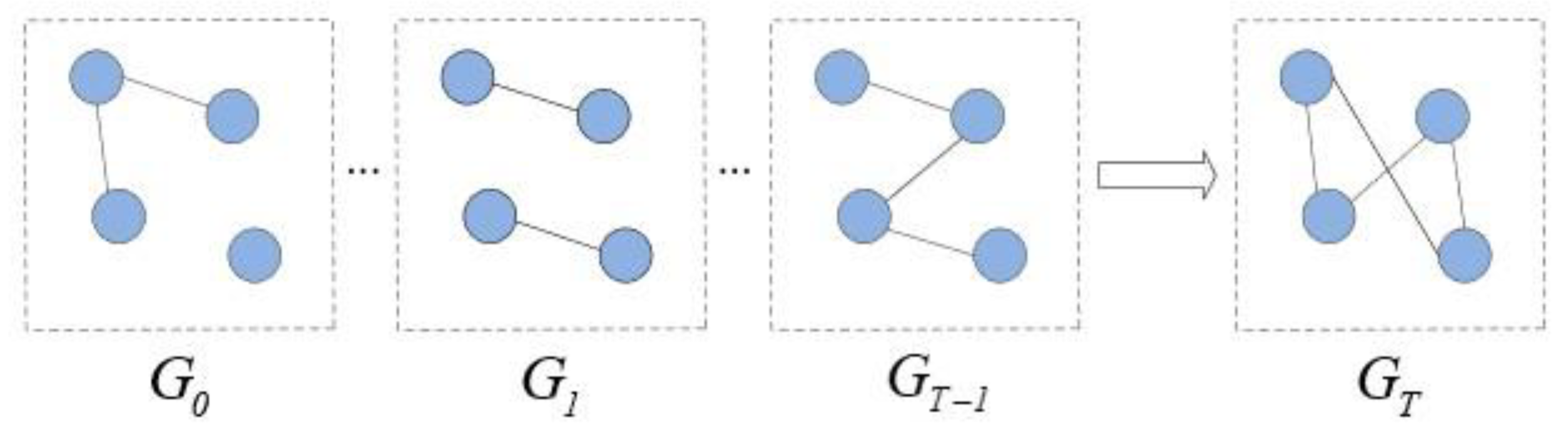
3.1. Problem Statement
3.2. Representation of Opportunistic Network
3.2.1. Topological Feature Representation
- (1)
- First-order adjacency matrix
- (2)
- Quadratic adjacency matrix
3.2.2. Attribute Feature Representation
3.2.3. State Matrix Construction
3.3. Link Prediction Model
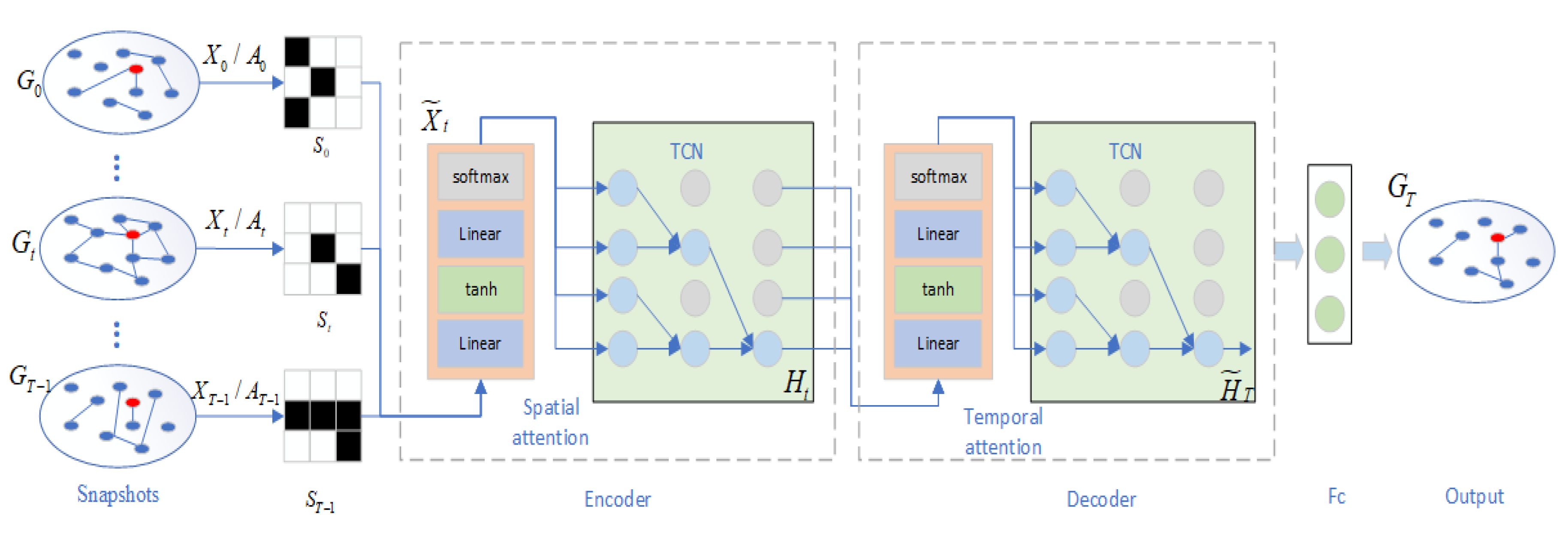
3.3.1. Overall Framework
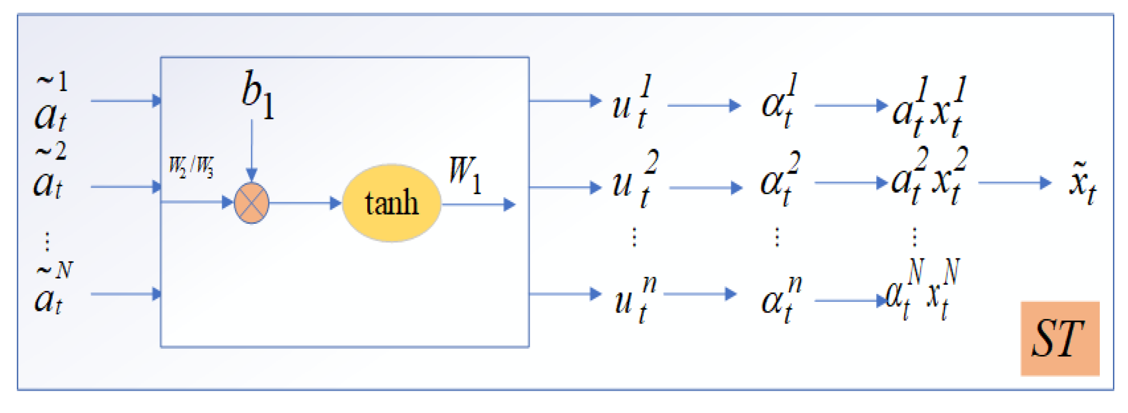
3.3.2. Spatial Attention-Based Encoder
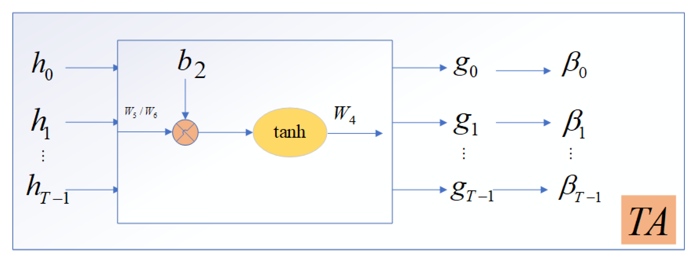
3.3.3. Temporal Attention-Based Decoder
3.3.4. Output and Loss Function
4. Experiments
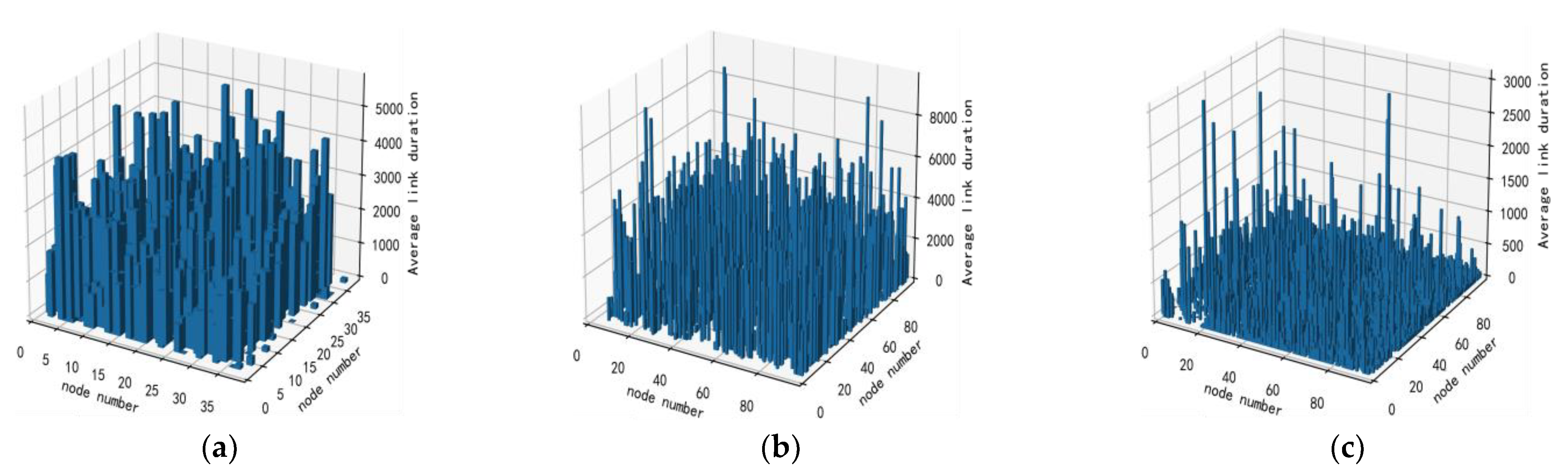
4.1. Datasets
4.2. Evaluate Metrics
- (1)
- Area Under the Curve (AUC) [26]: AUC is a widely used metric in binary classification that represents the area under the receiver operating characteristic (ROC) curve. The ROC curve is a plot of the true positive rate against the false positive rate at various threshold settings. AUC provides an overall measure of the model’s ability to discriminate between positive and negative classes.
- (2)
- Precision: Precision is defined as the proportion of correctly predicted links in a prediction list of all samples. It is calculated as the ratio of true positive predictions to the sum of true positive and false positive predictions.
- (3)
- F1-score: The single Precision is difficult to effectively evaluate, so a comprehensive evaluation metric F1-score is used as a supplement, which simultaneously considers the precision and recall of the classification model. Where recall is defined as the proportion of correctly predicted links in the test set.
4.3. Results and Analysis
4.3.1. Decision on Whether to Consider Link Frequency
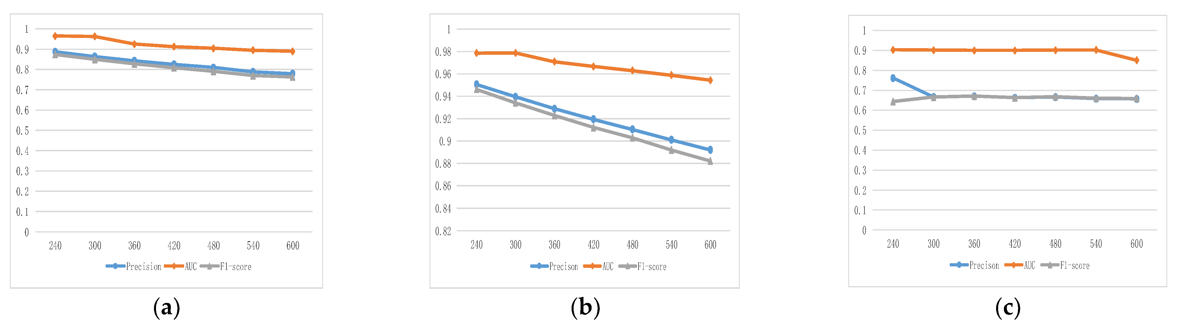
4.3.2. Determination of Slicing Size
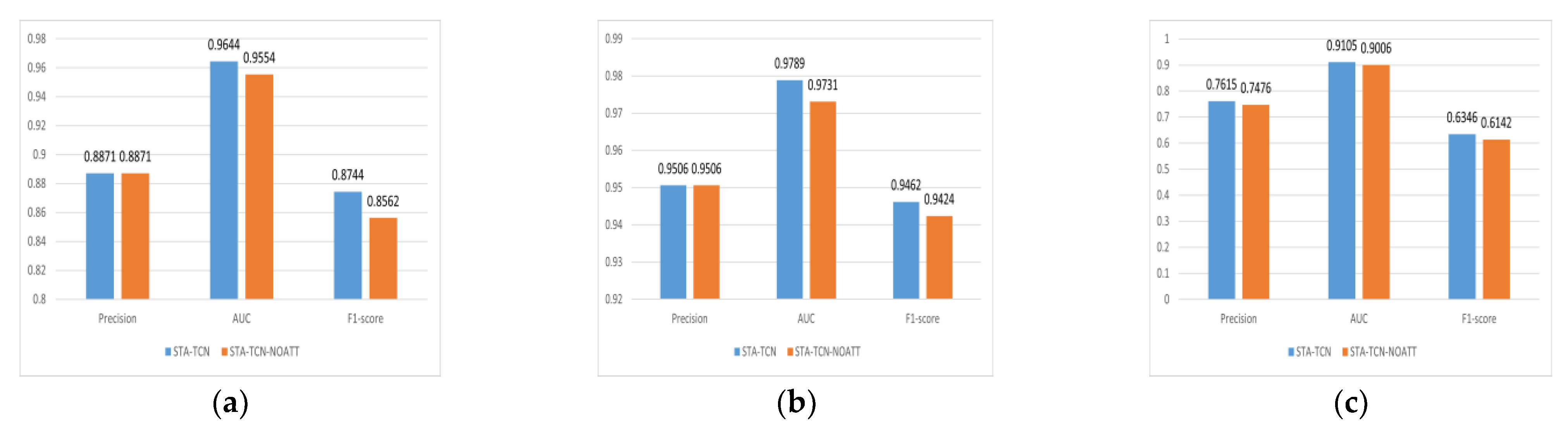
4.3.3. Validation of Spatial-Temporal Attention
4.3.4. Validation of Non-Autocorrelated Errors
4.3.5. Comparison of Link Prediction Performance
5. Conclusions
Author Contributions
Funding
Data Availability Statement
Conflicts of Interest
References
- Pirozmand, P.; Wu, G.; Jedari, B.; Xia, F. Human mobility in opportunistic networks: Characteristics, models and prediction methods. J. Netw. Comput. Appl. 2014, 42, 45–58. [Google Scholar] [CrossRef]
- Trifunovic, S.; Kouyoumdjieva, S.T.; Distl, B.; Pajevic, L.; Karlsson, G.; Plattner, B. A Decade of Research in Opportunistic Networks: Challenges, Relevance, and Future Directions. IEEE Commun. Mag. 2017, 55, 168–173. [Google Scholar] [CrossRef]
- Rajaei, A.; Chalmers, D.; Wakeman, I.; Parisis, G. Efficient Geocasting in Opportunistic Networks. Comput. Commun. 2018, 127, 105–121. [Google Scholar] [CrossRef]
- Avoussoukpo, C.B.; Ogunseyi, T.B.; Tchenagnon, M. Securing and Facilitating Communication within Opportunistic Networks: A Holistic Survey. IEEE Access 2021, 9, 55009–55035. [Google Scholar] [CrossRef]
- Xu, D.; Cheng, W.; Luo, D.; Liu, X.; Zhang, X. Spatio-Temporal Attentive RNN for Node Classification in Temporal Attributed Graphs. In Proceedings of the IJCAI’19, Macao, China, 10–16 August 2019; pp. 3947–3953. [Google Scholar]
- Sun, F.; Lang, C.; Boning, D. Adjusting for Autocorrelated Errors in Neural Networks for Time Series. In Proceedings of the Thirty-Fifth Conference on Neural Information Processing Systems, Online, 6–14 December 2021; pp. 29806–29819. [Google Scholar]
- Wang, W.; Feng, Y.; Jiao, P.; Yu, W. Kernel framework based on non-negative matrix factorization for networks reconstruction and link prediction. Knowl.-Based Syst. 2017, 137, 104–114. [Google Scholar] [CrossRef]
- Lv, L.; Bardou, D.; Hu, P.; Liu, Y.; Yu, G. Graph regularized nonnegative matrix factorization for link prediction in directed temporal networks using PageRank centrality. Chaos Solitons Fractals 2022, 159, 112107. [Google Scholar] [CrossRef]
- Nasiri, E.S.; Berahmand, K.; Li, Y. Robust graph regularization nonnegative matrix factorization for link prediction in attributed networks. Multimed. Tools Appl. 2022, 82, 3745–3768. [Google Scholar] [CrossRef]
- Gou, F.; Wu, J. Triad link prediction method based on the evolutionary analysis with IoT in opportunistic social networks. Comput. Commun. 2022, 181, 143–155. [Google Scholar] [CrossRef]
- Tran, C.; Shin, W.; Spitz, A.; Gertz, M. DeepNC: Deep Generative Network Completion. IEEE Trans. Pattern Anal. Mach. Intell. 2022, 44, 1837–1852. [Google Scholar] [CrossRef]
- Li, L.; Wen, Y.; Bai, S.; Liu, P. Link prediction in weighted networks via motif predictor. Knowl.-Based Syst. 2022, 242, 108402. [Google Scholar] [CrossRef]
- Huang, H.; Wei, Q.; Hu, M.; Feng, Y. Links Prediction Based on Hidden Naive Bayes Model. Adv. Eng. Sci. 2016, 48, 150–157. [Google Scholar]
- Shu, J.; Li, R.; Xiong, T.; Liu, L.; Sun, L. Link Prediction Based on Learning Automaton and Firefly Algorithm. Adv. Eng. Sci. 2021, 53, 133–140. [Google Scholar]
- Goyal, P.; Chhetri, S.R.; Canedo, A. dyngraph2vec: Capturing network dynamics using dynamic graph representation learning. Knowl.-Based Syst. 2020, 187, 104816. [Google Scholar] [CrossRef]
- Pareja, A.; Domeniconi, G.; Chen, J.; Ma, T.; Suzumura, T.; Kanezashi, H.; Kaler, T.; Leiserson, C.E. EvolveGCN: Evolving Graph Convolutional Networks for Dynamic Graphs. arXiv 2019, arXiv:1902.10191. [Google Scholar] [CrossRef]
- Chen, J.; Wang, X.; Xu, X. GC-LSTM: Graph convolution embedded LSTM for dynamic network link prediction. Appl. Intell. 2022, 52, 7513–7528. [Google Scholar] [CrossRef]
- Chen, J.; Zhang, J.; Xu, X.; Fu, C.; Zhang, D.; Zhang, Q.; Xuan, Q. E-LSTM-D: A Deep Learning Framework for Dynamic Network Link Prediction. IEEE Trans. Syst. Man Cybern. Syst. 2021, 51, 3699–3712. [Google Scholar] [CrossRef]
- Liu, L.; Yu, Z.; Zhu, H. A Link Prediction Method Based on Gated Recurrent Units for Mobile Social Network. J. Comput. Res. Dev. 2023, 60, 705–716. [Google Scholar]
- Yin, Y.; Wu, Y.; Yang, X.; Zhang, W.; Yuan, X. SE-GRU: Structure Embedded Gated Recurrent Unit Neural Networks for Temporal Link Prediction. IEEE Trans. Netw. Sci. Eng. 2022, 9, 2495–2509. [Google Scholar] [CrossRef]
- Bai, L.; Yao, L.; Li, C.; Wang, X.; Wang, C. Adaptive Graph Convolutional Recurrent Network for Traffic Forecasting. In Proceedings of the 34th International Conference on Neural Information Processing Systems, Vancouver, BC, Canada, 6–12 December 2020; pp. 17804–17815. [Google Scholar]
- Cirstea, R.; Kieu, T.; Guo, C.; Yang, B.; Pan, S.J. EnhanceNet: Plugin Neural Networks for Enhancing Correlated Time Series Forecasting. In Proceedings of the 2021 IEEE 37th International Conference on Data Engineering (ICDE), Chania, Greece, 19–22 April 2021; pp. 1739–1750. [Google Scholar]
- Guo, S.; Lin, Y.; Feng, N.; Song, C.; Wan, H. Attention Based Spatial-Temporal Graph Convolutional Networks for Traffic Flow Forecasting. In Proceedings of the Thirty-Third AAAI Conference on Artificial Intelligence and Thirty-First Innovative Applications of Artificial Intelligence Conference and Ninth AAAI Symposium on Educational Advances in Artificial Intelligence, Honolulu, HI, USA, 27 January–1 February 2019; pp. 922–929. [Google Scholar]
- Lea, C.; Flynn, M.D.; Vidal, R.; Reiter, A.; Hager, G.D. Temporal Convolutional Networks for Action Segmentation and Detection. In Proceedings of the IEEE Conference on Computer Vision and Pattern Recognition, Honolulu, HI, USA, 21–26 July 2017; pp. 1003–1012. [Google Scholar]
- Kotz, D.; Henderson, T. CRAWDAD: A Community Resource for Archiving Wireless Data at Dartmouth. IEEE Pervasive Comput. 2005, 4, 12–14. [Google Scholar] [CrossRef]
- Lü, L.; Zhou, T. Link prediction in complex networks: A survey. Phys. A Stat. Mech. Its Appl. 2011, 390, 1150–1170. [Google Scholar] [CrossRef]
- Shu, J.; Zhang, X.; Liu, L.; Yang, Z. Multi-nodes Link Prediction Method Based on Deep Convolution Neural Networks. Acta Electron. Sin. 2018, 46, 2970–2977. [Google Scholar]


| Dataset | ITC | MIT | Infocom06 |
|---|---|---|---|
| Data collection devices | iMote | Mobile phone | iMote |
| Number of nodes | 50 | 97 | 97 |
| Duration (day) | 12 | 246 | 3 |
| Type of communication | Bluetooth | Bluetooth | Bluetooth |
| Slicing Size (s) | ITC | MIT | Infocom06 |
|---|---|---|---|
| 240 | 86.67% | 70.67% | 10.77% |
| 300 | 85.28% | 64.85% | 7.33% |
| 360 | 84.24% | 58.64% | 5.14% |
| 420 | 82.50% | 52.07% | 3.77% |
| 480 | 82.03% | 46.14% | 2.78% |
| 540 | 81.80% | 40.89% | 2.10% |
| 600 | 72.76% | 36.40% | 1.68% |
| Methods | Dataset | ITC | MIT | Infocom06 | ||||||
|---|---|---|---|---|---|---|---|---|---|---|
| Metric | Precision | AUC | F1 | Precision | AUC | F1 | Precision | AUC | F1 | |
| TCN | 0.9123 | 0.9421 | 0.8684 | 0.9766 | 0.9755 | 0.9497 | 0.8165 | 0.8671 | 0.6121 | |
| LSTM | 0.9333 | 0.9625 | 0.885 | 0.9824 | 0.955 | 0.9108 | 0.7058 | 0.8953 | 0.6283 | |
| DynRNN [15] | 0.8312 | 0.9393 | 0.7869 | 0.927 | 0.9259 | 0.774 | 0.5057 | 0.829 | 0.4549 | |
| DynAERNN [15] | 0.9293 | 0.9582 | 0.8828 | 0.8858 | 0.8795 | 0.7046 | 0.5903 | 0.8574 | 0.5262 | |
| E-LSTM-D [18] | 0.9384 | 0.9592 | 0.8894 | 0.9494 | 0.9381 | 0.8483 | 0.7498 | 0.8927 | 0.6232 | |
| AGCRN [21] | 0.7702 | 0.9535 | 0.6454 | 0.9502 | 0.9235 | 0.7493 | 0.4769 | 0.8629 | 0.3903 | |
| STA-TCN | 0.8871 | 0.9644 | 0.8744 | 0.9506 | 0.9789 | 0.9462 | 0.7615 | 0.9105 | 0.6346 | |
Disclaimer/Publisher’s Note: The statements, opinions and data contained in all publications are solely those of the individual author(s) and contributor(s) and not of MDPI and/or the editor(s). MDPI and/or the editor(s) disclaim responsibility for any injury to people or property resulting from any ideas, methods, instructions or products referred to in the content. |
© 2024 by the authors. Licensee MDPI, Basel, Switzerland. This article is an open access article distributed under the terms and conditions of the Creative Commons Attribution (CC BY) license (https://creativecommons.org/licenses/by/4.0/).
Share and Cite
Shu, J.; Liao, Y.; Li, J. Spatial-Temporal Attention TCN-Based Link Prediction for Opportunistic Network. Electronics 2024, 13, 957. https://doi.org/10.3390/electronics13050957
Shu J, Liao Y, Li J. Spatial-Temporal Attention TCN-Based Link Prediction for Opportunistic Network. Electronics. 2024; 13(5):957. https://doi.org/10.3390/electronics13050957
Chicago/Turabian StyleShu, Jian, Yunchun Liao, and Jiahao Li. 2024. "Spatial-Temporal Attention TCN-Based Link Prediction for Opportunistic Network" Electronics 13, no. 5: 957. https://doi.org/10.3390/electronics13050957
APA StyleShu, J., Liao, Y., & Li, J. (2024). Spatial-Temporal Attention TCN-Based Link Prediction for Opportunistic Network. Electronics, 13(5), 957. https://doi.org/10.3390/electronics13050957