Abstract
Complex road environments threaten the safe operation of automated vehicles. Among these, adverse weather conditions and road geometries have particularly significant impacts. This study investigates LiDAR-based automated vehicles (LAVs) driving safety on vertical curved roads in adverse weather. A key methodology involves constructing a failure function that incorporates both the available sight distance (ASD) and the required stopping sight distance (RSD). This function is analyzed using a combined approach of neural networks and Monte Carlo simulations to quantitatively evaluate and generalize the reliability of LAVs under various conditions. The results reveal that variations in weather conditions and vertical curve radii significantly impact the ASD of LAVs, while the influence of speed is relatively minor. Notably, dense fog and rainfall can substantially reduce LAVs’ ASD on vertical curves. Furthermore, the vehicle automation level and speed have a significant impact on driving safety, emphasizing the need for road and operational domain design tailored to LAVs under adverse weather conditions and vertical curve radii.
1. Introduction
The International Society of Automotive Engineers (SAE) has categorized vehicles into automation levels ranging from Level 0 to Level 5 (L0 to L5), representing a spectrum from no automation to full automation. Over the past decade, automated vehicle (AV) technologies have flourished due to their potential to significantly improve safety and efficiency in road traffic [1,2,3,4]. However, complex road environments have become a threat in the application of AVs [5]. The primary challenges stem from adverse road geometry and weather conditions. Previous studies [5,6] have demonstrated that roads with small curvatures and weather conditions with low visibility can affect the perception accuracy of AVs. Particularly, since existing road geometric designs are mainly oriented toward human drivers, it becomes crucial to explore the safety of AVs operating in these complex road environments.
In recent years, many studies have assessed the adaptability of AVs to road geometries. Existing roads were designed for human drivers, catering to vehicles with no automation (L0). The safety evaluation of these roads for human-driven vehicles (HVs) primarily relies on the consistency of operating speeds. Current research utilizes advanced speed data collection methods to compare design speeds with operating speeds [7,8]. This approach identifies road sections that may pose higher risks, thereby promoting proactive road safety management. However, due to differences between AVs and human drivers, this method may no longer be applicable nor sufficient for exploring the coupling relationship between roads and AVs.
Therefore, it is essential to explore the coupling relationship between autonomous driving and roads. Researchers found that the primary distinction between AVs and HVs lies in the sight distance and lateral clearance. This difference is primarily attributed to the variance in perception-reaction time between the two types of vehicles [9,10]. Khoury et al. investigated the necessary changes in highway geometric design due to the transition to full AVs, emphasizing the revision of critical elements like stopping sight distance and decision sight distance [11]. García et al. analyzed the adaptation of semi-automated vehicles equipped with adaptive cruise control and lane-keeping assist systems to the horizontal alignment of 178 roads [12]. In addition to this, García also used the natural driving of AVs to explore the safe operating speed on existing roads [13]. Ye et al. investigated the impact of AVs on existing road design standards, including the adaptability in vertical curve design and the safety concerns at freeway entrances. The findings show that the required stopping sight distance (RSD) and the vertical curve length (LV) need to be considered for the operational safety of AVs [14]. Additionally, the research highlights safety issues at freeway entrances, noting that current designs may not provide adequate acceleration lane length and visibility for AVs. This suggests a pressing need to update road design standards to ensure AVs can operate safely and efficiently [15]. However, Wang et al. indicated that higher-level AVs (L4/L5) are capable of adapting to more challenging road geometries, whereas lower-level AVs, particularly those at Level 3, require more stringent road geometry standards [16,17,18]. Notably, these studies have provided substantial insights into the adaptability and safety of AVs in varied road geometries. Yet, there has been less focus on the safety of AV operations on specific road geometries under adverse weather conditions.
LiDAR is adopted as the prevalent perception solution for current AVs due to its stable performance, and its effectiveness in complex road environments directly influences the perceptual abilities of AVs. With the rapid development of LiDAR technology, the application of LiDAR-based AVs (LAVs) under adverse weather conditions has made significant progress. Byeon et al. utilized a custom-built LiDAR system, modeled in a virtual vehicle simulation, to examine how regional rain and fog droplet distributions affect LiDAR, revealing significant variations in signal attenuation and performance [19]. Wojtanowski et al. investigated the impact of environmental factors, such as visibility-dependent laser attenuation and variations in target reflectivity due to surface conditions, on the maximum range of laser rangefinders. They focused on devices operating at 905 nm and 1550 nm wavelengths, assessing their susceptibility to water-related environmental effects [20]. Natural driving tests were conducted to evaluate the effects of varying rainfall intensities on LiDAR parameters, such as distance, intensity, and point detection, revealing that increased rainfall significantly reduces LiDAR intensity and the number of detected points [21]. Research [22] presents a novel testing methodology for sensors and detection algorithms under different weather conditions, utilizing a sophisticated rain simulator with controllable layers to assess and quantify sensor robustness. Additionally, there are many studies focused on addressing the impact of atmospheric phenomena, such as rain and fog, on the performance of sensors [23,24]. Although these studies have enhanced our understanding of how adverse weather impacts LiDAR performance and assessed such impacts, they neglected the combined influences of adverse weather conditions and road geometries. Moreover, there is a gap in comprehensive simulation studies to account for challenging factors like unmanageable rainfall and curve radius, which are typically hard to control in field tests.
Furthermore, Olstam et al. have shown that road infrastructure and adverse weather significantly impact AVs [25]. Pappalardo et al. have investigated the operational design domain (ODD) of AVs’ lane support systems under various weather and road conditions. They identified crucial road and weather factors affecting the probability of LSS faults, proposed safe operational thresholds for LSS, and recommended the development of adaptive road design standards to accommodate autonomous driving technologies [26,27]. Hou et al. have evaluated the performance of mixed traffic, including HVs and connected AVs (CAVs) under adverse conditions. They found that a higher penetration rate of CAVs can improve both traffic efficiency and safety, particularly in adverse weather, indicating the potential advantages of integrating CAVs into the existing vehicle fleet [28]. While these studies evaluate AV safety in complex road environments, they often overlook the AV–road infrastructure relationship, focusing either on single systems or overall traffic flows.
Research on the safety of AVs in complex road settings has mostly been centered on the effects of specific weather conditions or road alignments at various AV levels. Nevertheless, there is a noticeable gap in evaluating how these factors jointly influence AVs’ sight distance. This study focuses on analyzing how LAV sight distance varies under different conditions, including challenging weather scenarios like rain and fog, a range of design speeds (Vd), and diverse vertical curve radii (RV). We plan to use reliability analysis for gauging the likelihood of sight distance failure in LAVs under adverse weather. The primary aim is to ascertain the driving safety of LAVs by examining their sight distance in multifaceted road environments.
2. Methods
This study evaluates the safety of LAVs on vertical curves in adverse weather, involving three steps: scenario design on a co-simulation platform, validation, and neural network-based risk assessment, as illustrated in Figure 1.
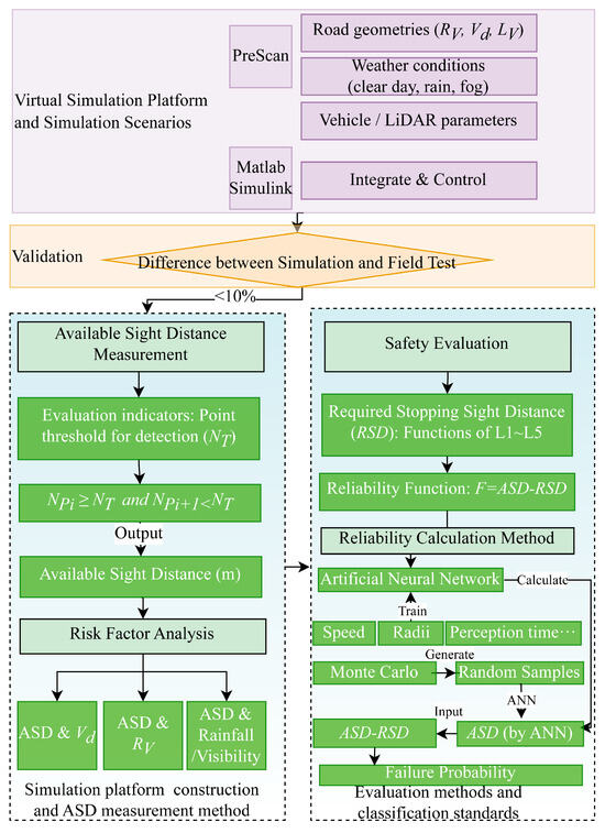
Figure 1.
Framework of this study.
2.1. Experimental Design
2.1.1. Simulation Platform and Scenarios
The integration of PreScan (version 2021.1.0) and Matlab-Simulink (version 2018b) on a co-simulation platform facilitates the creation and execution of various driving scenarios [17]. PreScan is responsible for providing detailed models of vehicles, roads with different geometrical shapes, and sensor simulations, including those for LiDAR systems. Matlab-Simulink complements this by enabling real-time access to critical simulation data, such as sensor outputs and vehicle trajectories, directly from PreScan. This combination allows for a comprehensive analysis of vehicle dynamics and sensor capabilities.
2.1.2. Vehicle Type and LiDAR Parameters
The Audi A8 was chosen as the experimental vehicle and LiDAR was employed as the AV’s sensor. Table 1 provides the LiDAR technical parameters and Figure 2 illustrates these parameters.

Table 1.
Typical/empirical values of LiDAR technical parameters selected in this study.
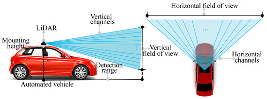
Figure 2.
LiDAR technical parameters.
- The laser wavelength has been set as 905 nm, bolstering its adaptability under adverse weather conditions. Current time-of-flight laser rangefinders typically use 905 nm and 1550 nm wavelengths: particularly, the shorter wavelength is less affected by weather [20], allowing for findings at this wavelength to be applied to other wavelength scenarios.
- The LiDAR was mounted on the vehicle’s roof to widen its vertical field of view and include extra vertical beams.
- The LiDAR point cloud threshold (NT) was configured at 10 to strike a balance between the accuracy of perception algorithms and the scenario modeling efficiency [17].
2.1.3. Design Speed
Typically, the ODD for AVs is required to exceed 40 km/h [18]. Moreover, when speeds exceed 100 km/h, traffic crashes are not directly related to the ASD [29]. Consequently, the study considers a speed range from 40 km/h to 100 km/h, increasing in 20 km/h increments.
2.1.4. Road Geometry
The configuration of road geometric parameters includes two parts: the tangent road and the vertical curve road, as illustrated in Figure 3.
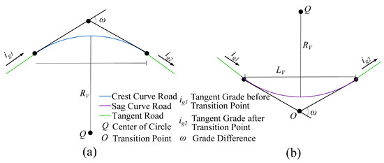
Figure 3.
Road geometry parameters: (a) crest curve; (b) sag curve.
- Tangent grade
A study [30] indicates that the tangent grade (ig) does not significantly impact ASD. Taking this into account, an ig of 4% is selected as it represents the upper limit for the design speed of 100 km/h [31]. Additionally, as shown by Equation (1), there is a proportional relationship between the radius (RV) and length (LV) of the vertical curve. To simplify the experimental setup and maintain a single variable control, we keep the grade difference |ω| constant. Specifically, before the transition point, the gradient is held at 0%. After the transition point, a fixed gradient of 4% is used for crest vertical curves and −4% for sag vertical curves. This approach standardizes the experimental conditions, ensuring simplicity and consistency in the setup.
where ω represents the grade difference, and a |ω| value of 4% is utilized to align with the chosen ig. LV is the vertical curve length; particularly, the LCV is the crest curve length and the LSV is the sag curve length. RV is the vertical curve radius, specifically, the RCV is the crest curve radius and the RSV is the sag curve radius.
LV = RV × ω
- Vertical curve
Parameter Range Selection: To comply with standards specified in the reference [31], the ranges for LCV (or LSV) and RCV (or RSV) are determined based on the |ω| of 4%. Furthermore, it is ensured that the minimum values of these ranges are not less than the prescribed limited minimum values (Llim_Vmin and Rlim_Vmin), and the maximum values are aligned with the common minimum values (Lcom_Vmin and Rcom_Vmin) specified by [31]. Additionally, the maximum values were set based on the common minimum values corresponding to the design speed of 100 km/h to enhance the comparability of the results. Table 2 lists this study’s vertical curve length and radius ranges.
Table 2.
Vertical curve radius ranges at selected design speed (|ω| = 4%).
2.1.5. Weather Conditions’ Parameters
Abdo et al. [32] have highlighted how rain and fog impair LiDAR’s ability to detect objects. Figure 4 depicts the theoretical variation of the laser attenuation coefficient. Typically, the intensity of rain and fog density are quantified using rainfall and visibility, respectively. Based on this, the laser attenuation coefficient is found to correlate positively with rain intensity but inversely with visibility. Notably, visibility impacts laser attenuation more significantly than rainfall. Further experimental investigations [33] indicate a substantial drop in LiDAR efficacy at a rainfall rate of 30 mm/h. Consequently, this study uses distinct levels of rainfall and visibility to evaluate their effects on LiDAR, detailed in Table 3.
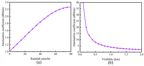
Figure 4.
Laser attenuation coefficients in adverse weather conditions: (a) rainfall; (b) visibility.
Table 3.
Parameters of the weather for simulation experiments.
Additionally, we made the following assumptions:
- Spherical droplets of rain and fog: Spherical droplets have been found to scatter lasers more effectively than other shapes [19]. Hence, this experiment assumed all rain and fog droplets are spherical.
- Randomness in laser–droplet interaction: The interaction between the laser beams and droplets is random, considering their trajectories and paths. As a result, this experimental model simplifies this by assuming a uniform distribution and consistent fall rate and speed for the droplets.
2.1.6. Available Sight Distance
While the LAV remains stationary on the initial position of vertical curves, the target vehicle (TV) moves away from it at a predetermined speed. The moment the LiDAR’s collected points (NP) drop below a threshold of NT = 10, the distance the TV has covered up to that point is recorded as the ASD, as shown in Figure 5.
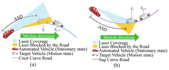
Figure 5.
Measurement of ASD: (a) crest curve; (b) sag curve.
2.2. Validation
The experimental platform and scenario validation were grounded on field tests by Abdo et al. [32]. Figure 6 presents the simulation and field test results of detection distances for different NT of stationary LiDAR on a tangent road under various weather conditions. In this comparison, the difference between the two results is not significant. This discrepancy could be attributed to measurement errors from LiDAR noise during field tests or differences in the cross-sectional areas of TV. Therefore, this virtual simulation approach is deemed viable for estimating ASDs in these scenarios.
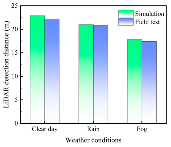
Figure 6.
Comparison of virtual simulation data with field test (NT = 10).
2.3. Risk Reliability Evaluation
2.3.1. Sight Distance Reliability Function
When establishing the sight distance reliability function to evaluate the road safety of AVs, the RSD plays a pivotal role. Previous studies [16] have established RSD calculation methods for AVs at various automation levels. These methods consider the differences between human drivers and automated systems, focusing on factors like perception-reaction time and longitudinal acceleration, as shown in Equations (2) and (3).
When the LAV’s automation level is L1/L2 or L4/L5, RSD is calculated by Equation (2):
When the LAV’s automation level is L3, RSD is calculated by Equation (3):
where RSD represents the required stopping sight distance, m. Vd denotes the design speed, km/h. Due to the RSD encounters safety concerns at speeds exceeding 60 km/h [30], the speed range studied in this paper is further narrowed down to 60–100 km/h. tPRT indicates the perception-reaction time, s; Axd represents the longitudinal braking deceleration, m/s2; Axdp is the predetermined longitudinal deceleration by the Level 3 automated system during the takeover time, m/s2; tTOT represents the time taken for a Level 3 driver to take over control, s; ig represents the road gradient, where it is positive for uphill and negative for downhill slopes.
Consequently, a situation where the AV’s RSD surpasses the ASD on the road is termed a sight distance failure. The correlation between these factors is measured by the sight distance reliability function (F), formulated through the following equation [30]:
where F was parameterized using artificial neural networks and Monte Carlo methods. F < 0 denotes a failure in sight distance, F = 0 signifies that the system is operating at its critical threshold, and F > 0 denotes reliable and safe sight distance.
F = ASD − RSD
2.3.2. Neural Network-Driven Parameter Estimation Methods
Due to the difficulty of determining the exact functional relationship between ASD and various influencing factors using traditional regression methods, we employ artificial neural networks (ANNs) to model complex nonlinear relationships [34].
Specifically, we compiled data from 2143 real vehicle tests and advanced driver-assistance systems (ADAS) databases, including information on design speed, perception-reaction time, longitudinal deceleration, road gradient, and weather conditions. We then designed a feedforward neural network with three hidden layers, each equipped with 128, 64, and 32 neurons, respectively, to progressively abstract and learn the high-level features of the input data. For the activation functions, we chose rectified linear unit (ReLU) for the hidden layers due to its effectiveness in accelerating neural network training, and the Sigmoid function for the output layer to ensure the output values ranged between 0 and 1, suitable for subsequent reliability assessment.
To train these ANNs, we standardized the ASD data and split it into two subsets for learning inference: 70% was allocated for training and 30% for validation. This division was guided by the standard practice to ensure both robust learning and effective validation of the model’s predictive capabilities [35].
Subsequently, we trained the network using the Adam optimizer with a learning rate of 0.001, chosen for its efficiency in handling large datasets. The mean squared error (MSE) was selected as the loss function to quantify the difference between the predicted visibility reliability and the actual values. To prevent overfitting, we implemented early stopping, and ceasing training if there was no improvement in the loss on the validation set over 10 consecutive training epochs.
This research assessed visibility reliability under different weather conditions using the Monte Carlo simulation method. By generating a large number of random samples representing various road conditions, vehicle speeds, and perception-reaction times, this method can estimate the probability of sight distance failure under specific conditions. In each simulation, a random sample was selected, and its corresponding sight distance reliability was calculated using the trained ANN model, thereby assessing the overall distribution of sight distance reliability.
The process is concluded as follows:
- (a)
- Initialize the neural network with specified structure and parameters.
- (b)
- Divide the dataset into 70% for training and 30% for validation.
- (c)
- Train the model using the training set until the early stopping criteria are met.
- (d)
- Generate random samples using the Monte Carlo method and calculate the ASD values using the trained ANN model.
- (e)
- Calculate the visibility reliability F value for each sample according to Equation (4).
- (f)
- Plot the simulation results to show the distribution of sight distance reliability under different conditions.
3. Results
3.1. Variations of Available Sight Distance
3.1.1. Variations of LAV’s ASD with Different Vertical Curve Radii and Speeds
The variations in ASD under different combinations of speeds and vertical curve radii are depicted in Figure 7. Figure 7a,b indicate that the ASD of LAV operating on crest and sag curves increases approximately linearly with the increase in the curve radius. Furthermore, it is observed that when the ASD reaches approximately 70 m, further enhancing the curve radius results in ASD fluctuating within a range of about 20 m. However, there is a difference between crest and sag curves in terms of ASD values. Particularly, the ASD eventually stabilizes at around 55 m with increasing radius on crest curves. In contrast, LAVs operating on sag curves experience ASD fluctuations within the range of 60 to 70 m.
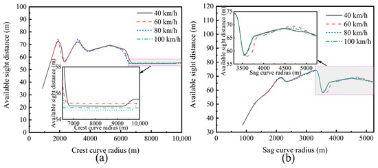
Figure 7.
The ASD of LAV operating on vertical curves: (a) Crest curves; (b) Sag curves.
Additionally, the results of LAV operating on crest and sag curves at different speeds show similar trends in ASD. Therefore, a speed of 80 km/h was selected for further analysis of ASD variations in adverse weather conditions.
3.1.2. Variation of LAV’s ASD on Vertical Curves under Different Weather Conditions
Figure 8 and Figure 9 show the variations in ASD for LAV operating on vertical curve roads under rainy and foggy conditions, respectively. As can be seen in Figure 8a,b, the ASD significantly decreases with increasing rainfall compared to clear day, regardless of whether they were operating on crest or sag curves. On average, the ASDs are reduced by approximately 2.5 to 3.0 m. Importantly, as rainfall intensifies further (or visibility correspondingly decreases), the rate of reduction in ASD shows a trend of gradual deceleration. This indicates that while initial rainfall significantly affects ASD, the additional impact of increased rainfall gradually weakens. Furthermore, the impact of the same amount of rainfall on LAVs’ ASD is somewhat diminished as the vertical curve radius increases.
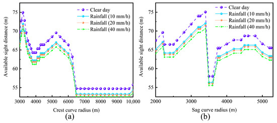
Figure 8.
The variations in ASD for LAV operating on vertical curve roads under rainy days: (a) crest curves; (b) sag curves.
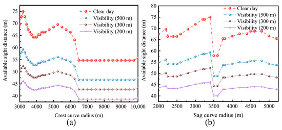
Figure 9.
The variations in ASD for LAV operating on vertical curve roads under foggy days: (a) crest curves; (b) sag curves.
Notably, the dense fog causes a greater decrease in LAVs’ ASD than rain, both on the crest and sag curves, as depicted in Figure 9a,b. Specifically, the ASD on different radii curves shortens by an average of 30 m as the visibility drops to 200 m. Moreover, the fog-related ASD reduction compared to clear days lessens with larger vertical curve radii, reaching an average difference of 25 m.
3.2. Evaluation of Sight Distance Failure Probability
Figure 10 and Figure 11 present the variations in sight distance failure probabilities of LAVs navigating on vertical curves under different vehicle automation levels, speeds, and weather conditions. Figure 10 illustrates that the level of vehicle automation significantly affects the sight distance failure probability of LAVs on crest vertical curves. Specifically, the L3 LAV exhibits the highest probability of sight distance failure at consistent speeds (as shown in Figure 10b,e,h), followed by the L1/L2 LAV (Figure 10a,d,g), while the L4/L5 LAV demonstrate the lowest probability (Figure 10c,f,i). Moreover, an increase in speed correlates with a higher sight distance failure probability for all vehicle automation levels, and all automation levels exceed 5% at speeds of 80–100 km/h.
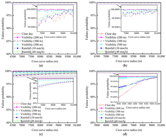
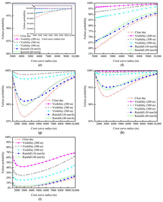
Figure 10.
Sight distance failure probability of LAVs driving on crest curve roads at varying radii, speeds, and weather conditions: (a) L1/L2 LAV drives at 100 km/h; (b) L3 LAV drives at 100 km/h; (c) L4/L5 LAV drives at 100 km/h; (d) L1/L2 LAV drives at 80 km/h; (e) L3 LAV drives at 80 km/h; (f) L4/L5 LAV drives at 80 km/h; (g) L1/L2 LAV drives at 60 km/h; (h) L3 LAV drives at 60 km/h; (i) L4/L5 LAV drives at 60 km/h.
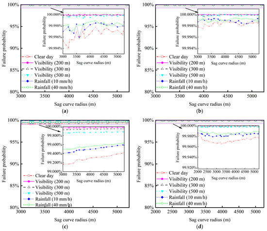
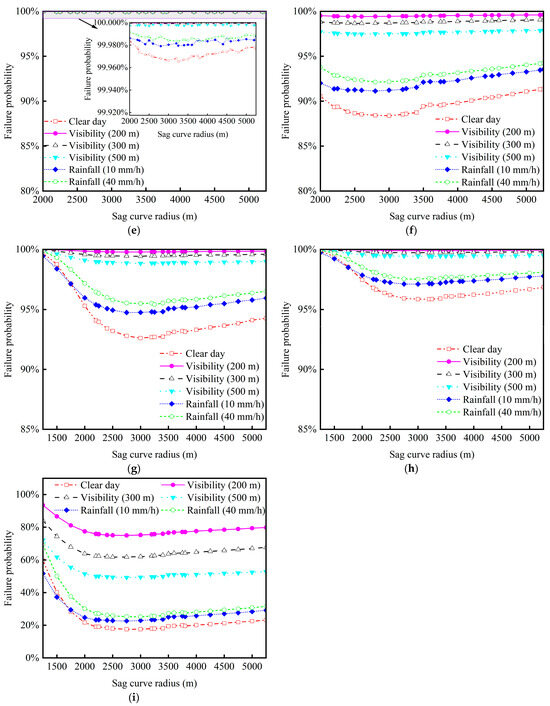
Figure 11.
Sight distance failure probability of LAVs driving on sag curve roads at varying radii, speeds, and weather conditions: (a) L1/L2 LAV drives at 100 km/h; (b) L3 LAV drives at 100 km/h; (c) L4/L5 LAV drives at 100 km/h; (d) L1/L2 LAV drives at 80 km/h; (e) L3 LAV drives at 80 km/h; (f) L4/L5 LAV drives at 80 km/h; (g) L1/L2 LAV drives at 60 km/h; (h) L3 LAV drives at 60 km/h; (i) L4/L5 LAV drives at 60 km/h.
The relationship between sight distance failure probability and the vertical curve radius displays a specific trend. In particular, on clear days or days with rainfall under 40 mm/h, LAV sight distance failure probability drops below 5% and then rises above 5% as the crest vertical curve radius increases, reaching a turning point at around 2500 m. Notably, only the L4/L5 LAV maintains a sight distance failure probability below 5% at 60 km/h in clear day or light rain conditions within a curve radius of around 2500 m. Furthermore, rainfall intensity and fog visibility levels augment the probability of sight distance failure across all conditions, with fog having a significantly greater impact than rainfall. For instance, under the situations depicted in Figure 10i, a visibility of 200 m markedly increases the risk of sight distance failure by approximately 50% compared to clear days.
Similarly, as demonstrated in Figure 11, the sight distance failure probability of LAVs is influenced by automation level, speed, and weather conditions for sag curves, following a pattern similar to that of crest curves. However, the sight distance failure probability generally exceeds 5% in sag curves. Even in the situation consisting of a clear day and 60 km/h, the probability decreases by 60% compared to a visibility of 200 m but still surpasses the 95% safety reliability threshold, as shown in Figure 11i.
4. Discussion
This study focused on the variations in ASD for LiDAR-based AV under different operating conditions, assessing the safety of LAVs on existing vertical curve roads. These conditions include various speeds, vertical curve radii, and different weather scenarios. The results aim to deepen the understanding of the dynamic interplay between operational parameters of AVs and road safety, guiding road design oriented to AVs.
Specifically, while navigating on both crest and sag curves, the LAV’s ASD initially increases linearly as the curve radius expands, but this trend is followed by fluctuations and eventual stabilization. This phenomenon is attributed to the fact that smaller vertical curve radii correspond to shorter curve lengths, causing the LAV’s ASD to increase as the curve radius expands. However, when the curve radius enlarges beyond LiDAR’s perceptual range, trends in ASD gradually align with that on horizontal tangent roads, consistent with Wang’s findings [18]. Furthermore, the cruising angle of the LAV on vertical curves varies due to changes in the relative position between the LAV and TV, which is the primary cause of fluctuations in ASD. Significantly, there is a variance in stable ASD values between crest and sag curves, which deviates from the findings in [30]. More precisely, the ASD fluctuates around 55 m on crest curves, in contrast to 60 to 70 m observed on sag curves. This variation results from the laser beams’ interaction with the environment, as shown in Figure 5. Actually, most laser beams emitted by LAVs are absorbed by the air on crest curves, while they predominantly illuminate the road on sag curves, leading to a greater ASD. Intriguingly, speed does not significantly impact the ASD of LAVs operating on vertical curves, this is consistent with the findings of [30]. This is because this study fixed the gradient at 4%, which led to minor changes in both the gradient and the cruising angle in the vertical profile. Consequently, there are no significant changes in the cruising angle even at higher speeds, suggesting that speed does not notably influence ASD.
Adverse weather conditions also significantly affect the LAV’s ASD. Compared to clear days, ASD significantly decreases with increasing rainfall or reduced visibility in foggy conditions. It is noteworthy that dense fog has a greater impact on ASD than rain, aligning with the research [19,24]. This is attributed to the interaction of raindrops and fog particles with laser beams. Raindrops primarily scatter the beams, whereas fog particles, being much smaller, cause more frequent absorption and scattering. This difference results in a reduced number of laser pulses returning to the sensor.
Furthermore, the vehicle’s automation level and speed are the dominant factors influencing safe operation, consistent with previous studies [12,14,30]. Although there is a low correlation between the LAV’s ASD and speed, the implication of higher speeds leading to longer RSD increases the failure probability. Similarly, the RSD becomes greater when the perception-reaction times related to automation levels increase, thereby elevating the risk associated with vehicle operation.
The probability of sight distance failure initially increases and then decreases as the vertical curve radius enlarges, with a critical point at approximately 2500 m. This is mainly because a radius less than 2500 m leads to the ASD exceeding the curve length, reducing sight distance failure risk. Conversely, the curve becomes more tangent-like when the radius exceeds 2500 m, which shortens the path in the AV’s LiDAR field, leading to reduced ASD and increased risk.
High-level automated LAVs can meet safety and reliability standards only when operating on crest curves under conditions of clear visibility and low speed. This is mainly because adverse weather conditions weaken the ASD, and high speeds and sag curves demand a greater RSD. As a result, it is essential to redesign the operational domain of LAVs for existing roads, encompassing measures such as decreasing their speed and refraining from utilizing them in adverse weather conditions to ensure safe driving.
5. Conclusions
This study presents an analysis of the impact of ASD when LAVs of different automation levels navigate through existing vertical curves under various weather conditions. Our findings elucidate the dynamic relationship between vehicle speed, vertical curve radii, weather conditions, and the vehicle automation level, highlighting their collective influence on road safety for LAVs.
- Influence of Curve Radius and Speed on ASD: We observed that ASD increases linearly with the curve radius expansion for both crest and sag curves up to a certain point, beyond which it stabilizes or fluctuates within a small range. This phenomenon underscores the importance of optimizing vertical curve radii in road design to enhance the operational efficiency of LAVs without compromising safety. The impact of speed on ASD was found to be less significant, suggesting that road geometry plays a more crucial role in determining sight distance than vehicle speed within the tested range.
- Adverse Weather Conditions: The study confirms that adverse weather conditions substantially reduce ASD. Fog presents a more severe reduction in ASD than rain, necessitating the consideration of weather adaptability in both vehicle automation level control and road infrastructure planning. This finding calls for adaptive speed limits and enhanced weather prediction integration within autonomous vehicle systems to mitigate visibility-related risks.
- Sight Distance Failure Probability: Our analysis reveals a nuanced relationship between sight distance failure probability and various factors, including automation level, speed, and curve radius. High-level automation (L4/L5) vehicles demonstrate a lower probability of sight distance failure under optimal conditions (clear days and lower speeds), which deteriorates with adverse weather. This highlights the critical need for incorporating robust perception systems in LAVs that can adapt to changing environmental conditions and maintain safety.
- Policy and Design Implications: The findings advocate for a reevaluation of current road design standards to facilitate AVs. Additionally, ensuring safety on existing roads may require adjustments in speed limits based on weather conditions and vertical curve characteristics.
- Limitations and Future Work: This study evaluated the safety of LAVs driving on vertical curves from the perspective of sight distance safety. Although this evaluation provides a perspective for understanding the safe operation of LAVs, we plan to broaden our research scope in future work. Specifically, we will assess the dynamic performance of AVs to comprehensively examine their safety and comfort during operation. Moreover, considering that snowy conditions have a greater impact on road friction performance than on visibility, we will also include the effects of snowy conditions in our analysis of dynamic performance.
Author Contributions
Conceptualization, M.C. and C.M.; Data curation, C.M. and W.Z.; Formal analysis, M.C.; Investigation, C.M.; Methodology, M.C. and C.M.; Resources, M.C.; Software, W.Z.; Supervision, B.Y.; Validation, M.C., C.M. and W.Z.; Visualization, M.C.; Writing—original draft, M.C.; Writing—review and editing, B.Y. All authors have read and agreed to the published version of the manuscript.
Funding
This research was funded by the National Natural Science Foundation of China, grant number 51878163.
Data Availability Statement
All data, models, or code that support the findings of this study are available from the corresponding author upon reasonable request.
Conflicts of Interest
Chengyang Mao was employed by Wuxi Transportation Construction Engineering Group Co., Ltd. Wen Zhou was employed by Guangzhou Urban Planning & Design Survey Research Institute Co., Ltd. The remaining authors declare that the research was conducted in the absence of any commercial or financial relationships that could be construed as a potential conflict of interest.
References
- Alam, A.; Besselink, B.; Turri, V.; Mårtensson, J.; Johansson, K.H. Heavy-Duty Vehicle Platooning for Sustainable Freight Transportation: A Cooperative Method to Enhance Safety and Efficiency. IEEE Control Syst. 2015, 35, 34–56. [Google Scholar] [CrossRef]
- Virdi, N.; Grzybowska, H.; Waller, S.T.; Dixit, V. A Safety Assessment of Mixed Fleets with Connected and Autonomous Vehicles Using the Surrogate Safety Assessment Module. Accid. Anal. Prev. 2019, 131, 95–111. [Google Scholar] [CrossRef]
- Amirgholy, M.; Shahabi, M.; Oliver Gao, H. Traffic Automation and Lane Management for Communicant, Autonomous, and Human-Driven Vehicles. Transp. Res. Part C Emerg. Technol. 2020, 111, 477–495. [Google Scholar] [CrossRef]
- Novat, N.; Kidando, E.; Kutela, B.; Kitali, A.E. A Comparative Study of Collision Types between Automated and Conventional Vehicles Using Bayesian Probabilistic Inferences. J. Saf. Res. 2023, 84, 251–260. [Google Scholar] [CrossRef]
- Chai, C.; Liu, T.; Liu, J.; Cao, X.; Hu, Y.; Li, Q. Surrogate Evaluation Model for Assessing Lane Detection Reliability of Automated Vehicles in Complex Road Environments. Transp. Res. Rec. J. Transp. Res. Board 2023, 2677, 185–195. [Google Scholar] [CrossRef]
- Haselhoff, A.; Kummert, A. 2D Line Filters for Vision-Based Lane Detection and Tracking. In Proceedings of the 2009 International Workshop on Multidimensional (nD) Systems, Thessaloniki, Greece, 29 June–1 July 2009; IEEE: Piscataway, NJ, USA, 2009; pp. 1–5. [Google Scholar]
- Serrone, G.D.; Cantisani, G.; Peluso, P. Speed Data Collection Methods: A Review. Transp. Res. Procedia 2023, 69, 512–519. [Google Scholar] [CrossRef]
- Serrone, G.D.; Cantisani, G.; Peluso, P.; Coppa, I.; Mancinetti, M.; Bianchini, B. Road Infrastructure Safety Management: Proactive Safety Tools to Evaluate Potential Conditions of Risk. Transp. Res. Procedia 2023, 69, 711–718. [Google Scholar] [CrossRef]
- Naujoks, F.; Höfling, S.; Purucker, C.; Zeeb, K. From Partial and High Automation to Manual Driving: Relationship between Non-Driving Related Tasks, Drowsiness and Take-over Performance. Accid. Anal. Prev. 2018, 121, 28–42. [Google Scholar] [CrossRef] [PubMed]
- Atwood, J.R.; Guo, F.; Blanco, M. Evaluate Driver Response to Active Warning System in Level-2 Automated Vehicles. Accid. Anal. Prev. 2019, 128, 132–138. [Google Scholar] [CrossRef] [PubMed]
- Khoury, J.; Amine, K.; Abi Saad, R. An Initial Investigation of the Effects of a Fully Automated Vehicle Fleet on Geometric Design. J. Adv. Transp. 2019, 2019, 6126408. [Google Scholar] [CrossRef]
- García, A.; Camacho-Torregrosa, F.J.; Padovani Baez, P.V. Examining the Effect of Road Horizontal Alignment on the Speed of Semi-Automated Vehicles. Accid. Anal. Prev. 2020, 146, 105732. [Google Scholar] [CrossRef]
- García, A.; Camacho-Torregrosa, F.J. Influence of Lane Width on Semi- Autonomous Vehicle Performance. Transp. Res. Rec. 2020, 2674, 279–286. [Google Scholar] [CrossRef]
- Ye, X.; Wang, X.; Liu, S.; Tarko, A.P. Feasibility Study of Highway Alignment Design Controls for Autonomous Vehicles. Accid. Anal. Prev. 2021, 159, 106252. [Google Scholar] [CrossRef]
- Ye, X. Operational Design Domain of Automated Vehicles at Freeway Entrance Terminals. Accid. Anal. Prev. 2022, 174, 106776. [Google Scholar] [CrossRef]
- Wang, S.; Yu, B.; Ma, Y.; Liu, J.; Zhou, W. Impacts of Different Driving Automation Levels on Highway Geometric Design from the Perspective of Trucks. J. Adv. Transp. 2021, 2021, 5541878. [Google Scholar] [CrossRef]
- Wang, S.; Ma, Y.; Liu, J.; Yu, B.; Zhu, F. Readiness of As-Built Horizontal Curved Roads for LiDAR-Based Automated Vehicles: A Virtual Simulation Analysis. Accid. Anal. Prev. 2022, 174, 106762. [Google Scholar] [CrossRef] [PubMed]
- Wang, S.; Mao, C.; Ma, Y.; Liu, J.; Yu, B. Examining the Feasibility of Current Spiral Curve Design Controls for LiDAR-based Automated Vehicles. IET Intell. Trans. Syst. 2022, 17, 848–866. [Google Scholar] [CrossRef]
- Byeon, M.; Yoon, S.W. Analysis of Automotive Lidar Sensor Model Considering Scattering Effects in Regional Rain Environments. IEEE Access 2020, 8, 102669–102679. [Google Scholar] [CrossRef]
- Wojtanowski, J.; Zygmunt, M.; Kaszczuk, M.; Mierczyk, Z.; Muzal, M. Comparison of 905 Nm and 1550 Nm Semiconductor Laser Rangefinders’ Performance Deterioration Due to Adverse Environmental Conditions. Opto-Electron. Rev. 2014, 22, 183–190. [Google Scholar] [CrossRef]
- Filgueira, A.; González-Jorge, H.; Lagüela, S.; Díaz-Vilariño, L.; Arias, P. Quantifying the Influence of Rain in LiDAR Performance. Measurement 2017, 95, 143–148. [Google Scholar] [CrossRef]
- Hasirlioglu, S.; Kamann, A.; Doric, I.; Brandmeier, T. Test Methodology for Rain Influence on Automotive Surround Sensors. In Proceedings of the 2016 IEEE 19th International Conference on Intelligent Transportation Systems (ITSC), Rio de Janeiro, Brazil, 1–4 November 2016; IEEE: Piscataway, NJ, USA, 2016; pp. 2242–2247. [Google Scholar]
- Rasshofer, R.H.; Spies, M.; Spies, H. Influences of Weather Phenomena on Automotive Laser Radar Systems. Adv. Radio Sci. 2011, 9, 49–60. [Google Scholar] [CrossRef]
- Hasirlioglu, S.; Riener, A. Introduction to Rain and Fog Attenuation on Automotive Surround Sensors. In Proceedings of the 2017 IEEE 20th International Conference on Intelligent Transportation Systems (ITSC), Yokohama, Japan, 16–19 October 2017; IEEE: Piscataway, NJ, USA, 2017; pp. 1–7. [Google Scholar]
- Olstam, J.; Johansson, F.; Alessandrini, A.; Sukennik, P.; Lohmiller, J.; Friedrich, M. An Approach for Handling Uncertainties Related to Behaviour and Vehicle Mixes in Traffic Simulation Experiments with Automated Vehicles. J. Adv. Transp. 2020, 2020, 8850591. [Google Scholar] [CrossRef]
- Pappalardo, G.; Caponetto, R.; Varrica, R.; Cafiso, S. Assessing the Operational Design Domain of Lane Support System for Automated Vehicles in Different Weather and Road Conditions. J. Traffic Transp. Eng. (Engl. Ed.) 2022, 9, 631–644. [Google Scholar] [CrossRef]
- Cafiso, S.; Pappalardo, G. Safety Effectiveness and Performance of Lane Support Systems for Driving Assistance and Automation—Experimental Test and Logistic Regression for Rare Events. Accid. Anal. Prev. 2020, 148, 105791. [Google Scholar] [CrossRef] [PubMed]
- Hou, G. Evaluating Efficiency and Safety of Mixed Traffic with Connected and Autonomous Vehicles in Adverse Weather. Sustainability 2023, 15, 3138. [Google Scholar] [CrossRef]
- Ma, Y.; Easa, S.; Cheng, J.; Yu, B. Automatic Framework for Detecting Obstacles Restricting 3D Highway Sight Distance Using Mobile Laser Scanning Data. J. Comput. Civ. Eng. 2021, 35, 04021008. [Google Scholar] [CrossRef]
- Wang, S.; Ma, Y.; Easa, S.M.; Zhou, H.; Lai, Y.; Chen, W. Sight Distance of Automated Vehicle Considering Highway Vertical Alignments and Its Implications for Speed Limits. IEEE Intell. Transp. Syst. Mag. 2023, 1–18. [Google Scholar] [CrossRef]
- JTG D20-2017; Ministry of Transport of the People’s Republic of China (MTPRC) Design Specification for Highway Alignment. China Communications Press Co., Ltd.: Beijing, China, 2017.
- Abdo, J.; Hamblin, S.; Chen, G. Effective Range Assessment of Lidar Imaging Systems for Autonomous Vehicles Under Adverse Weather Conditions ith Stationary Vehicles. ASCE-ASME J. Risk Uncert. Engrg. Syst. Part B Mech. Engrg. 2022, 8, 031103. [Google Scholar] [CrossRef]
- Suganuma, N.; Yoshioka, M.; Yoneda, K.; Aldibaja, M. LIDAR-Based Object Classification for Autonomous Driving on Urban Roads. Autom. Robot. 2017, 3, 92–95. [Google Scholar]
- Ostad-Ali-Askari, K.; Shayannejad, M.; Ghorbanizadeh-Kharazi, H. Artificial Neural Network for Modeling Nitrate Pollution of Groundwater in Marginal Area of Zayandeh-Rood River, Isfahan, Iran. KSCE J. Civ. Eng. 2017, 21, 134–140. [Google Scholar] [CrossRef]
- Afram, A.; Janabi-Sharifi, F.; Fung, A.S.; Raahemifar, K. Artificial Neural Network (ANN) Based Model Predictive Control (MPC) and Optimization of HVAC Systems: A State of the Art Review and Case Study of a Residential HVAC System. Energy Build. 2017, 141, 96–113. [Google Scholar] [CrossRef]
Disclaimer/Publisher’s Note: The statements, opinions and data contained in all publications are solely those of the individual author(s) and contributor(s) and not of MDPI and/or the editor(s). MDPI and/or the editor(s) disclaim responsibility for any injury to people or property resulting from any ideas, methods, instructions or products referred to in the content. |
© 2024 by the authors. Licensee MDPI, Basel, Switzerland. This article is an open access article distributed under the terms and conditions of the Creative Commons Attribution (CC BY) license (https://creativecommons.org/licenses/by/4.0/).