
An Improved Safety Belt Detection Algorithm for High-Altitude Work Based on YOLOv8


Abstract
1. Introduction
2. Related Work
3. Methods
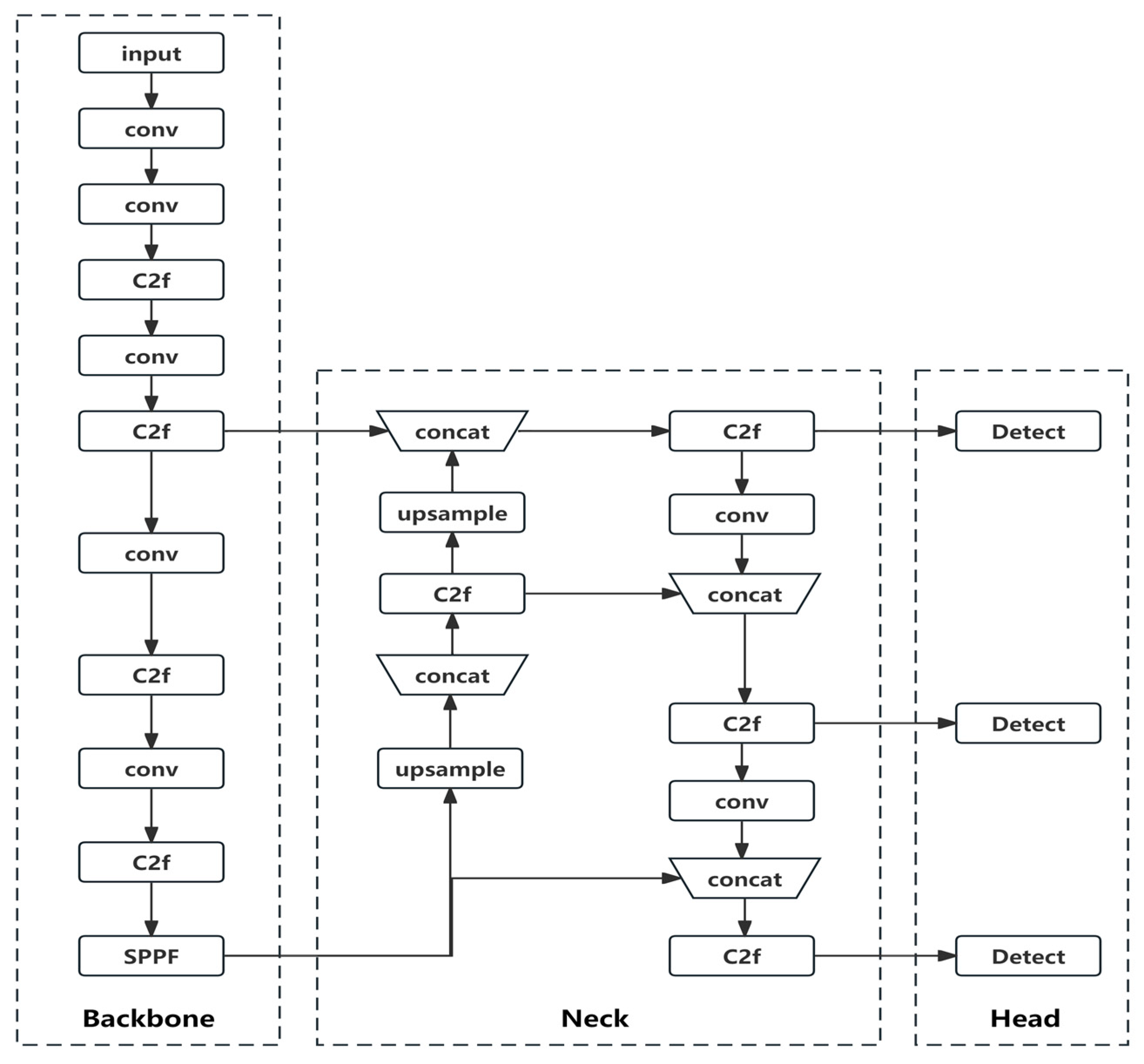
3.1. YOLOv8 Model
- Backbone: The Backbone layer is a network responsible for feature extraction. Its main role is to extract relevant information from images, which can then be utilized by subsequent networks or modules for further processing and analysis.
- Neck: The Neck layer is positioned between the Backbone and the Head to optimize the utilization of features extracted by the backbone. It plays a crucial role in feature fusion, enabling the Neck layer to effectively combine and integrate the extracted features.
- Head: The Head layer utilizes the previously extracted features to perform recognition.
3.2. Improvement Measures
- Occlusion by Other Objects: During high-altitude electrical work, there can be other objects that occlude the visibility of safety belts worn by electricians.
- Misidentification of Cables: Aerial cables and similar structures in high-altitude electrical work can be mistakenly identified as safety belts, leading to inaccurate detection results.
- Variations in Lighting Conditions and Electrician Movements: The dynamic changes in lighting conditions and the movement of electricians during high-altitude operations introduce complexities in accurately detecting safety belts.
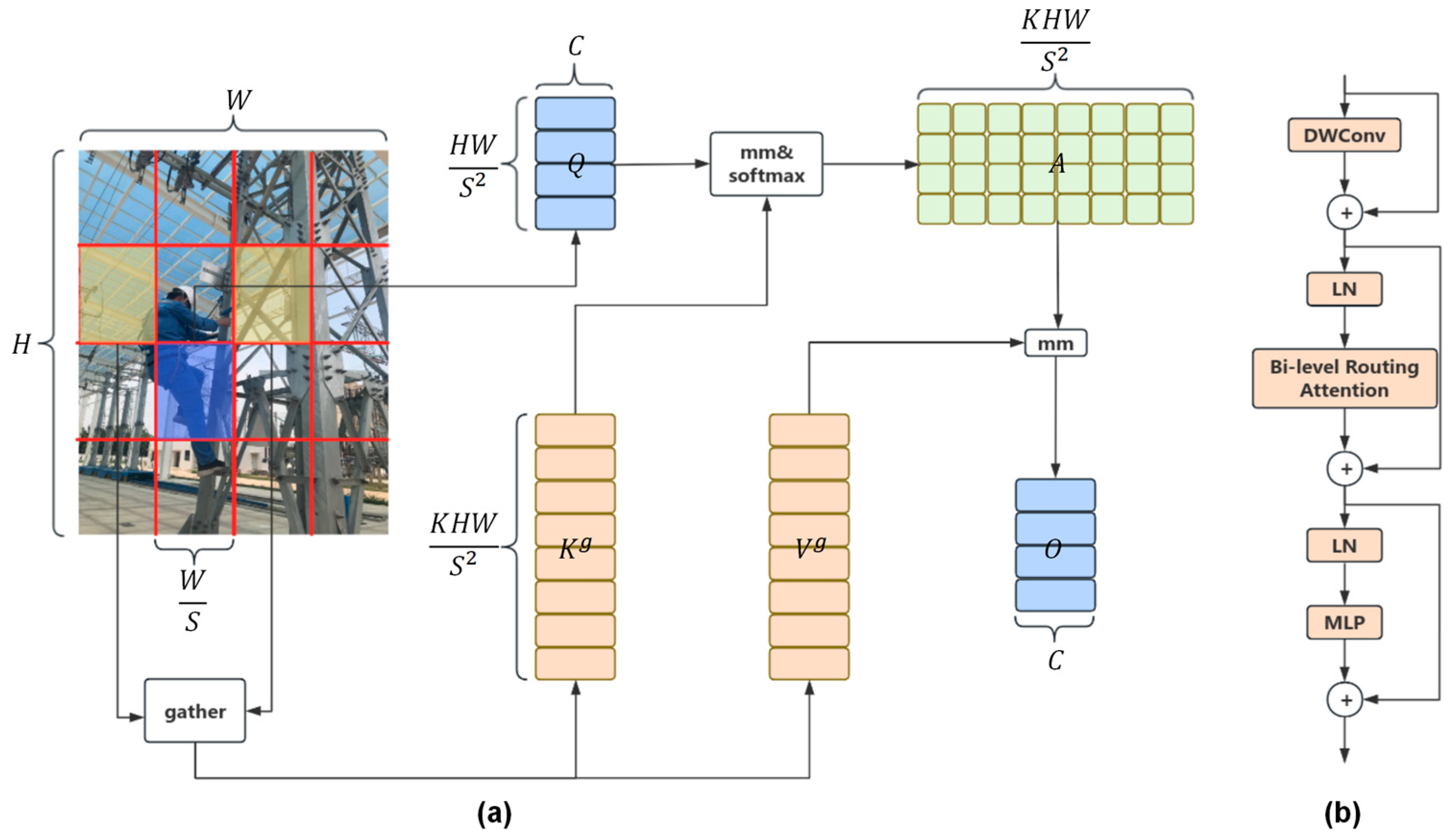
- Firstly, an attention mechanism is integrated into the Backbone layer to enhance the capability of feature extraction. Through multiple experimental trials, attention mechanisms, known as Biformer, are introduced at various locations within the Backbone layer. After careful evaluation, it is determined that adding Biformer attention at the end of the Backbone layer yields the most favorable results. This choice is made considering that incorporating attention mechanisms in the shallower layers of the Backbone layer would lead to increased computational complexity.
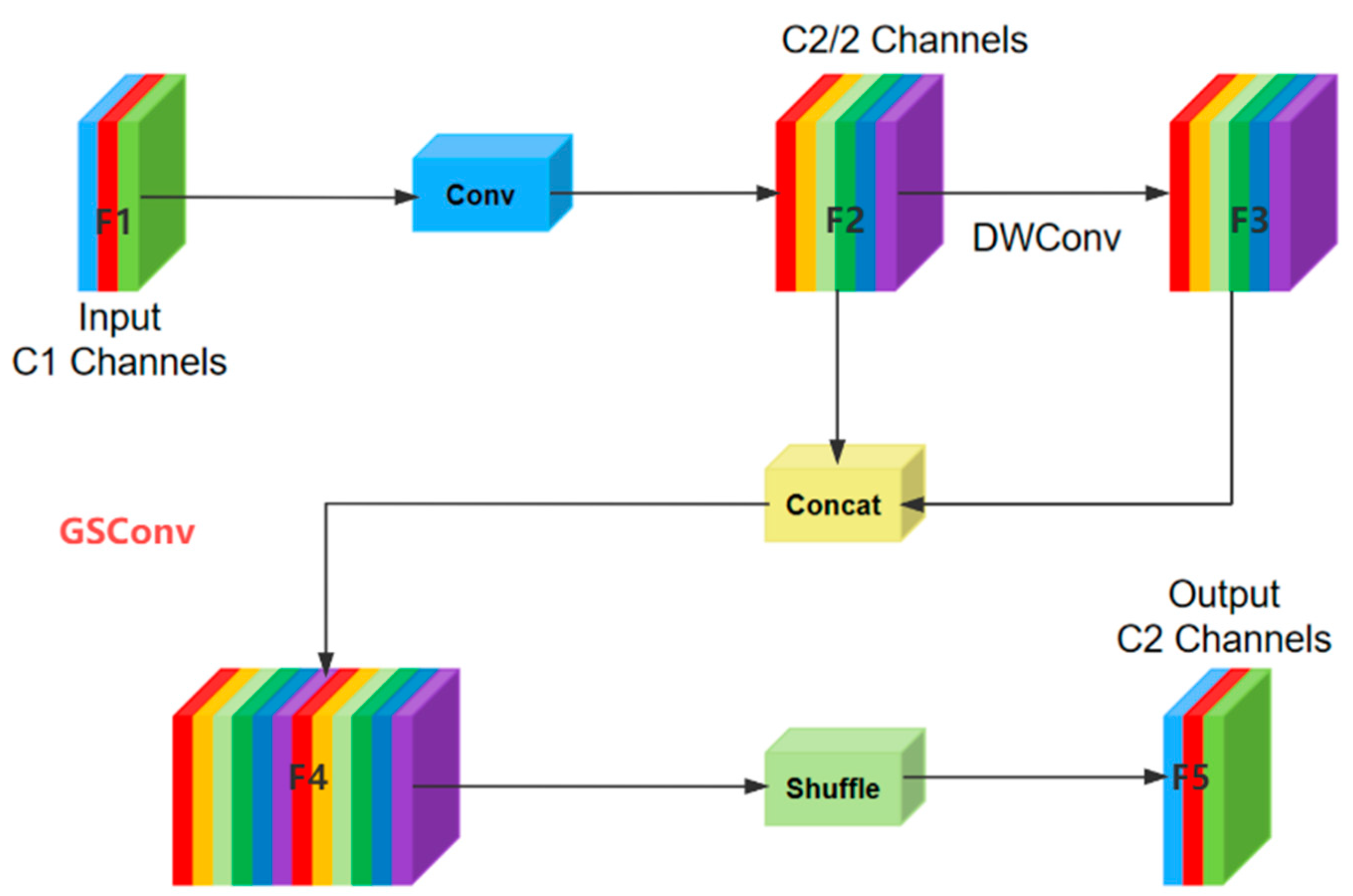
- Secondly, in the Neck layer, the original upsampling operations are completely replaced with the CARAFE lightweight upsampling operator. Additionally, a lightweight network called Slim-neck is employed as the neck structure to maintain the network’s performance while reducing the model complexity and making it more lightweight. The C2f module is replaced with the VoVGSCSP module, and all 3 × 3 convolutions are substituted with GSConv.
- Thirdly, additional auxiliary heads are incorporated into the Head layer to facilitate training and enable the intermediate layers of the network to learn more information.
- Lastly, the original loss function is replaced with the MPDIoU loss function, which optimizes the regression of bounding boxes. This replacement aims to improve the accuracy and precision of object detection.
3.2.1. Biformer Attention
- Partitioning Regions and Linear Mapping:
- 2.
- Implementing Inter-Region Routing via Directed Graphs:
- 3.
- Token-to-token Attention:
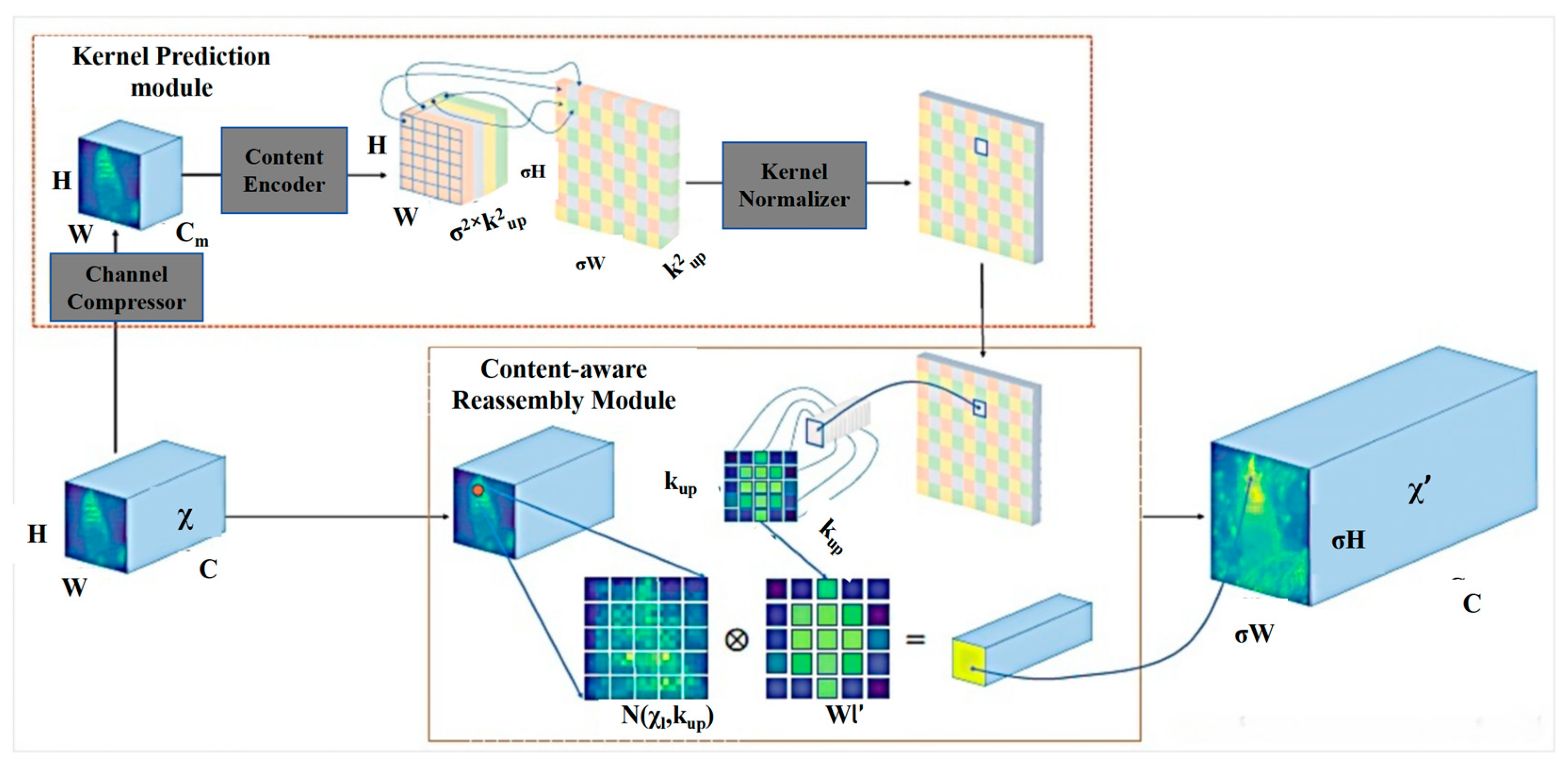
3.2.2. Lightweight Upsampling Operator CARAFE
- (1)
- The upsampling kernel prediction module:
- (2)
- The content-aware reassembly module:
3.2.3. Slim-Neck
3.2.4. Auxiliary Training Heads
3.2.5. Improvement of the Loss Function
4. Experiments and Analysis
4.1. Experimental Setting
4.2. Dataset
4.3. Evaluation Metrics
4.4. Comparative Analysis and Experimental Results
4.4.1. The Ablation Experiments
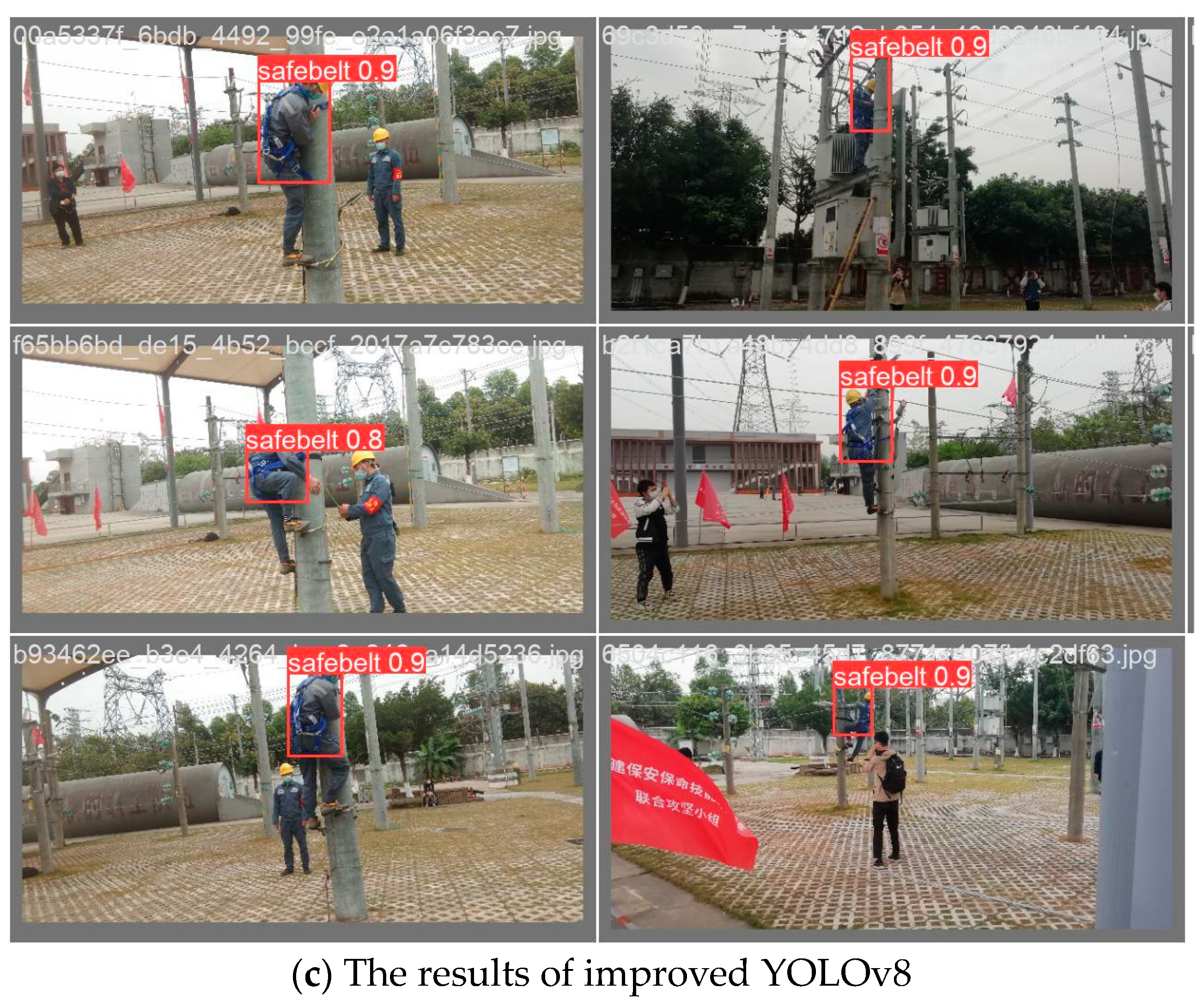
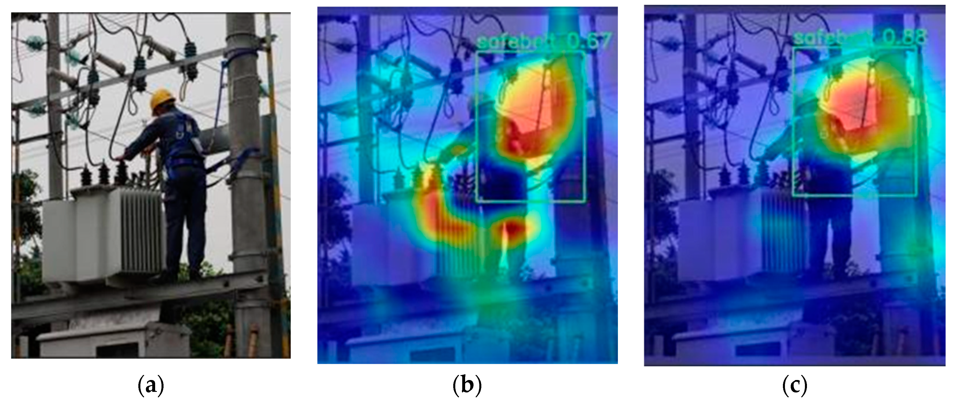
4.4.2. Test the Effect of The Experimental Pictures
5. Conclusions
Author Contributions
Funding
Data Availability Statement
Conflicts of Interest
References
- Sun, S.; Zhao, J.; Fu, G. Study on behavioral causes of falling accidents based on “2-4” model. China Saf. Sci. J. 2019, 29, 23–28. [Google Scholar]
- Diwan, T.; Anirudh, G.; Tembhurne, J.V. Object detection using YOLO: Challenges, architectural successors, datasets and applications. Multimed. Tools Appl. 2023, 82, 9243–9275. [Google Scholar] [CrossRef] [PubMed]
- Deng, J.; Xuan, X.; Wang, W.; Li, Z.; Yao, H.; Wang, Z. A review of research on object detection based on deep learning. J. Phys. Conf. Ser. 2020, 1684, 012028. [Google Scholar] [CrossRef]
- Hebbache, L.; Amirkhani, D.; Allili, M.S.; Hammouche, N.; Lapointe, J.-F. Leveraging Saliency in Single-Stage Multi-Label Concrete Defect Detection Using Unmanned Aerial Vehicle Imagery. Remote Sens. 2023, 15, 1218. [Google Scholar] [CrossRef]
- Girshick, R.; Donahue, J.; Darrell, T.; Malik, J. Rich feature hierarchies for accurate object detection and semantic segmentation. In Proceedings of the IEEE Conference on Computer Vision and Pattern Recognition, Columbus, OH, USA, 23–28 June 2014; pp. 580–587. [Google Scholar]
- Girshick, R. Fast R-CNN. In Proceedings of the IEEE Conference on Computer Vision and Pattern Recognition, Santiago, Chile, 7–13 December 2015; pp. 1440–1448. [Google Scholar]
- Ren, S.; He, K.; Girshick, R.; Sun, J. Faster r-cnn: Towards real-time object detection with region proposal networks. Adv. Neural Inf. Process. Syst. 2015, 28, 91–99. [Google Scholar] [CrossRef] [PubMed]
- He, K.; Gkioxari, G.; Dollár, P.; Girshick, R. Mask R-CNN. IEEE Trans. Pattern Anal. Mach. Intell. 2020, 42, 386–397. [Google Scholar] [CrossRef] [PubMed]
- Wang, T.; Anwer, R.M.; Cholakkal, H.; Khan, F.S.; Pang, Y.; Shao, L. Learning rich features at high-speed for single-shot object detection. In Proceedings of the 2019 IEEE/CVF International Conference on Computer Vision, Seoul, Republic of Korea, 27 October–2 November 2019; pp. 1971–1980. [Google Scholar]
- Liu, W.; Anguelov, D.; Erhan, D.; Szegedy, C.; Reed, S.; Fu, C.Y.; Berg, A.C. SSD: Single shot multibox detector. In Proceedings of the 14th European Conference on Computer Vision, Amsterdam, The Netherland, 11–14 October 2016; pp. 21–37. [Google Scholar]
- Redmon, J.; Divvala, S.; Girshick, R.; Farhadi, A. You only look once: Unified, real-time object detection. In Proceedings of the IEEE Conference on Computer Vision and Pattern Recognition, Las Vegas, NV, USA, 27–30 June 2016; pp. 779–788. [Google Scholar]
- Redmon, J.; Farhadi, A. YOLO9000: Better, faster, stronger. In Proceedings of the IEEE Conference on Computer Vision and Pattern Recognition, Honolulu, HI, USA, 21–26 July 2017; pp. 7263–7271. [Google Scholar]
- Redmon, J.; Farhadi, A. Yolov3: An incremental improvement. arXiv 2018, arXiv:1804.02767. [Google Scholar]
- Bochkovskiy, A.; Wang, C.Y.; Liao, H.Y.M. Yolov4: Optimal speed and accuracy of object detection. arXiv 2020, arXiv:2004.10934. [Google Scholar]
- Mseddi, W.S.; Ghali, R.; Jmal, M.; Attia, R. Fire detection and segmentation using YOLOv5 and U-net. In Proceedings of the 2021 29th European Signal Processing Conference (EUSIPCO), Dublin, Ireland, 23–27 August 2021; pp. 741–745. [Google Scholar]
- Chen, Q.; Wang, Y.; Yang, T.; Zhang, X.; Cheng, J.; Sun, J. You only look one-level feature. In Proceedings of the IEEE Conference on Computer Vision and Pattern Recognition, Virtual, 19–25 June 2021; pp. 13034–13043. [Google Scholar]
- Wang, C.Y.; Bochkovskiy, A.; Liao, H.Y.M. YOLOv7: Trainable bag-of-freebies sets new state-of-the-art for real-time object detectors. In Proceedings of the IEEE Conference on Computer Vision and Pattern Recognition, Vancouver, BC, Canada, 17–24 June 2023; pp. 7464–7475. [Google Scholar]
- Reis, D.; Kupec, J.; Hong, J.; Daoudi, A. Real-Time Flying Object Detection with YOLOv8. arXiv 2023, arXiv:2305.09972. [Google Scholar]
- Terven, J.; Cordova-Esparza, D. A comprehensive review of YOLO: From YOLOv1 to YOLOv8 and beyond. arXiv 2023, arXiv:2304.00501. [Google Scholar]
- Feng, Z.; Zhang, W.; Zheng, Z. High-altitude operating seat belt detection based on Mask R-CNN. Comput. Syst. Appl. 2021, 30, 202–207. (In Chinese) [Google Scholar]
- Zhang, M.; Han, Y.; Liu, Z. Detection method of high-altitude safety protective equipment for construction workers based on deep learning. China Saf. Sci. J. (CSSJ) 2022, 32, 140–146. (In Chinese) [Google Scholar]
- Cao, J.; Guo, Z.B.; Pan, L.Z. Detection of Safety Belt Wearing in Aerial Work. J. Hum. Univ. Sci. (Nat. Sci. Ed.) 2022, 37, 92–99. (In Chinese) [Google Scholar]
- Zhu, L.; Wang, X.; Ke, Z.; Zhang, W.; Lau, R.W. BiFormer: Vision Transformer with Bi-Level Routing Attention. In Proceedings of the IEEE/CVF Conference on Computer Vision and Pattern Recognition, Vancouver, BC, Canada, 17–24 June 2023; pp. 10323–10333. [Google Scholar]
- Gao, X.; Tang, Z.; Deng, Y.; Hu, S.; Zhao, H.; Zhou, G. HSSNet: A end-to-end network for detecting tiny targets of apple leaf diseases in complex backgrounds. Plants 2023, 12, 2806. [Google Scholar] [CrossRef] [PubMed]
- Wang, J.; Chen, K.; Xu, R.; Liu, Z.; Loy, C.C.; Lin, D. Carafe: Content-aware reassembly of features. In Proceedings of the IEEE/CVF International Conference on Computer Vision, Long Beach, CA, USA, 16–20 June 2019; pp. 3007–3016. [Google Scholar]
- Li, H.; Li, J.; Wei, H.; Liu, Z.; Zhan, Z.; Ren, Q. Slim-neck by GSConv: A better design paradigm of detector architectures for autonomous vehicles. arXiv 2022, arXiv:2206.02424. [Google Scholar]
- Ma, S.; Xu, Y. MPDIoU: A Loss for Efficient and Accurate Bounding Box Regression. arXiv 2023, arXiv:2307.07662. [Google Scholar]


| Name | Configure |
|---|---|
| Operating system | Windows 10 |
| Processor | Intel(R) Xeon(R) W-2255 CPU @ 3.70GHz |
| Video card | NVIDIA GeForce RTX 3080Ti |
| Run memory | 64GB |
| GPU internal storage | 12GB |
| Programming tools | Pycharm |
| Programming language | python |
| Deep learning framework | Pytorch2.0.0 |
| Parameter | Value |
|---|---|
| Learning | 0.01 |
| Batch Size | 4 |
| Epochs | 300 |
| Workers | 4 |
| Model | Precision/% | Recall/% | mAP@0.5/% | mAP@0.5:0.95% | Flops/G | Model Size/MB |
|---|---|---|---|---|---|---|
| before | 0.929 | 0.909 | 0.962 | 0.765 | 8.1 | 5.9 |
| after | 0.98 | 0914 | 0.973 | 0.781 | 7.6 | 7.8 |
| Model | Precision/% | Recall/% | mAP@0.5/% | Flops/G | Model Size/MB |
|---|---|---|---|---|---|
| yolov7-tiny | 0.947 | 0.845 | 0.895 | 13 | 11.7 |
| yolov5s | 0.968 | 0.938 | 0.959 | 16.3 | 14.4 |
| yolov8 | 0.929 | 0.909 | 0.962 | 8.1 | 5.9 |
| yolov8 + Biformer | 0.956 | 0.938 | 0.965 | 8.1 | 6.8 |
| yolov8 + TripleAttention | 0.908 | 0.938 | 0.957 | 8.1 | 6.2 |
| yolov8 + Biformer + CARAFE + slim | 0.944 | 0.93 | 0.968 | 7.6 | 6.4 |
| yolov8 + Biformer + CARAFE + slim + Aux | 0.949 | 0.92 | 0.969 | 7.6 | 7.8 |
| yolov8 + Biformer + CARAFE + slim + Aux + mpdiou | 0.98 | 0.914 | 0.973 | 7.6 | 7.8 |
| yolov8 + Biformer + CARAFE + dyhead | 0.964 | 0.926 | 0.971 | 9.8 | 7.9 |
| yolov8 + Biformer + CARAFE + bifpn + Aux | 0.942 | 0.91 | 0.969 | 7.4 | 6.1 |
| yolov8 + Biformer + CARAFE + bifpn + Aux + mpdiou | 0.944 | 0.908 | 0.967 | 7.4 | 6.1 |
Disclaimer/Publisher’s Note: The statements, opinions and data contained in all publications are solely those of the individual author(s) and contributor(s) and not of MDPI and/or the editor(s). MDPI and/or the editor(s) disclaim responsibility for any injury to people or property resulting from any ideas, methods, instructions or products referred to in the content. |
© 2024 by the authors. Licensee MDPI, Basel, Switzerland. This article is an open access article distributed under the terms and conditions of the Creative Commons Attribution (CC BY) license (https://creativecommons.org/licenses/by/4.0/).
Share and Cite
Jiang, T.; Li, Z.; Zhao, J.; An, C.; Tan, H.; Wang, C. An Improved Safety Belt Detection Algorithm for High-Altitude Work Based on YOLOv8. Electronics 2024, 13, 850. https://doi.org/10.3390/electronics13050850
Jiang T, Li Z, Zhao J, An C, Tan H, Wang C. An Improved Safety Belt Detection Algorithm for High-Altitude Work Based on YOLOv8. Electronics. 2024; 13(5):850. https://doi.org/10.3390/electronics13050850
Chicago/Turabian StyleJiang, Tingyao, Zhao Li, Jian Zhao, Chaoguang An, Hao Tan, and Chunliang Wang. 2024. "An Improved Safety Belt Detection Algorithm for High-Altitude Work Based on YOLOv8" Electronics 13, no. 5: 850. https://doi.org/10.3390/electronics13050850
APA StyleJiang, T., Li, Z., Zhao, J., An, C., Tan, H., & Wang, C. (2024). An Improved Safety Belt Detection Algorithm for High-Altitude Work Based on YOLOv8. Electronics, 13(5), 850. https://doi.org/10.3390/electronics13050850