Abstract
The use of machine learning (ML) and its applications is one of the leading research areas nowadays. Neural networks have recently gained enormous popularity and many works in various fields use them in the hope of improving previous results. The application of the artificial intelligence (AI) methods and the rationale for this decision is one issue, but the assessment of such a model is a completely different matter. People mostly use mean square error or less often mean absolute error in the absolute or percentage versions. One should remember that an error does not equal an error and a single value does not provide enough knowledge about the causes of some behavior. Proper interpretation of the results is crucial. It leads to further model improvement. It might be challenging, but allows us to obtain better and more robust solutions, which ultimately solve real-life problems. The ML model assessment is the multicriteria task. A single measure delivers only a fraction of the picture. This paper aims at filling that research gap. Commonly used integral measures are compared with alternative measures like factors of the Gaussian and non-Gaussian statistics, robust statistical estimators, tail index and the fractional order. The proposed methodology delivers new single-criteria indexes or the multicriteria approach, which extend the statistical concept of the moment ratio diagram (MRD) into the index ratio diagram (IRD). The proposed approach is validated using real data from the Full Truck Load cost estimation example. It compares 35 different ML regression algorithms applied to that task. The analysis gives an insight into the properties of the selected methods, enables their comparison and homogeneity analysis and ultimately leads towards constructive suggestions for their eventual proper use. The paper proposes new indexes and concludes that correct selection of the residuum analysis methodology makes the assessment and the ML regression credible.
1. Introduction
Full truck loads (FTL) is a common transportation method, where the goods fill an entire truck. It perfectly suits a large volume of goods, where a load covers the whole truck space. Apart from the FTL, there exists an alternative method called less-than truckload (LTL), in which a truck takes several partial loads to different contract load/unload locations within a single journey. This work focuses on the FTL, however from a rarely addressed perspective.
In case of the external fleet contract pricing, the contracts are priced according to the varying contractor policy, which takes into account several objective and subjective market and non-market factors [1,2], such as contract0dependent, economic, regulatory, general and purely ambivalent factors. Those factors potentially reflect, in the opinion of the decision maker, the shipping cost for a given commodity, along some determined route within a certain time period. Dynamic pricing shows increasing shipping business dynamics [3] and determines it simultaneously [4]. Next, it is assumed the contractor may use some custom dynamic pricing model, which is associated with serious challenges [5].
The shipping cost estimations start to play an even more important role in case of short routes, when common relations between the price, fuel costs and the driver time is not straightway included. The pricing of the FTL long-range contracts is frequently solved using deterministic analytical fright calculators [6], or with the use of algorithmic estimators. It is worth noting that the AI and ML methods [7] lead in that area. The literature mostly focuses on the blind machine learning approaches [2,8,9,10] or hybrid ones [11].
On the contrary, the task of the short-range FTL shipment cost estimation, i.e., for routes shorter than 50 km, is seldom addressed in the literature. One may try to determine the reasons for that. Firstly, this task is of a smaller order and is often hidden in all data, or omitted due to the lower absolute cost values of such routes. Secondly, these routes often play a complementary or secondary role in relation to the long-distance ones. Thirdly, it is a thankless and simply difficult task. The fact that we undertake this task is related to its difficulty and observations made while dealing with the general task of estimating FTL costs [11], where the largest relative errors occur precisely for short routes, which spoils the overall picture of the modeling and estimation task.
The multi-criteria assessment methodology is the second contribution of this work. It is a well-known fact that each performance index, such as means square error, absolute error or various residuum statistical factors, exhibit different properties and are sensitive towards different estimation error aspects. Despite that knowledge, there is a significant deficiency in the literature, because multi-criteria residuum assessment approaches are hardly reported [12]. The researchers mostly use the mean square error (MSE), mean absolute error (MAE) or the relative mean absolute percentage error (MAPE). Each of them has different properties and puts more attention on various data features. Square errors are sensitive to large residua, while even often-occurring but small errors are neglected. Absolute errors equalize these differences and reflect small residua as well.
During this research, different measures are investigated: classical (normal), robust and L-moments, tail index and the Geweke-Porter-Hudak estimator of the fractional order of the ARFIMA filter. They are presented following the statistical approach named moment ratio diagrams (MRD) or L-moments ratio diagram (LMRD). Our work plans to supplement the estimation residuum analysis with the multi-criteria approach named the IRD—(Index Ratio Diagrams) using various measures.
The main contribution of this work lies in the proposal of the multicriteria residuum analysis concept, as this aspect is hardly existent in the research. The FTL estimation task is considered as the representative example for the assessment methodology.
General FTL cost estimation task formulation is introduced in Section 2, while Section 3 describes the utilized assessment methods and estimation algorithms. Various estimators are compared in Section 4. Section 5 presents the results of the multi-criteria residuum analysis, while Section 6 concludes the paper.
2. Estimation Case Study
The analysis uses the data from selected Polish shipping companies [9]. The original database consists of approximately 414,000 records. Once the data are limited only to the short-range contracts, the number of records is limited to 20,239 from 1 January 2016 till 30 April 2022. These data are used for training. Contracts from 1 May 2022 till 1 August 2022 (703 records) are used for validation, as shown in Table 1.

Table 1.
Number of records used during the analysis.
Data Preprocessing and Features Selection
Each contract included in the database is characterized by 22 independent features. We limit this number to the 12 most important variables listed in Table 2. This table does not include an important feature like the fuel cost, which is highly volatile due to varying geopolitical and economic situations. The following descriptors are excluded from the estimation process:

Table 2.
The list of selected features.
- ID number—a sequence number;
- Maximum weight and tonne-kilometers, as they are frequently incomplete;
- Geographical clusters [11], the latitudes and longitudes of the loading and unloading places, which are used only in the selection of the short-range routes.
Python programming language (scikit_learn and torch libraries) and MATLAB (Statistics and Machine Learning Toolbox) are used during data processing and the estimation process.
3. Methods and Algorithms
This research uses quite a large scope of possible methods, which are included in the proposed IRD framework: integral indexes, classical, robust and L-moments, tail index and the Geweke–Porter–Hudak fractional order estimator of the ARFIMA filter. Methods used during calculations are described below.
3.1. Integral Measures
The MSE measure is calculated as the mean integral of the squared residua over some time period
It penalizes large errors, neglecting the smaller ones. This measure is significantly affected by outlying occurrences and exhibits the zero-breakdown point [13]. The MAE index sums absolute residua values
The MAE is less conservative as it penalizes continuing small residua. Though its breakdown point is zero as well, it is robust against a portion of outliers. The MAPE is defined in a relative way:
Generally, it is difficult to define what error value is good and which model is proper enough. Lewis, in [14], proposed the interpretation of typical MAPE values, which is presented in Table 3.

Table 3.
Interpretations of MAPE values.
3.2. Statistical Moments
This research follows a theoretical approach that assumes some distribution, which correctly represents the underlying process. Such probabilistic density function (PDF) is utilized through their factors and moments (if they exist).
Let us assume that is a given time series with the mean and the r-th central moment , denotes the expectation. The mean is the first moment , and the variance is the second one denoted as , where denotes the standard deviation. These moments are often used together with the third one, i.e., the skewness and the fourth—the kurtosis . The skewness reflects data asymmetry and kurtosis its concentration.
The existence of outlying observations in the time series causes its distributions to start to be fat-tailed [15]. This feature biases the moments estimation. The use of statistical factors in the residuum analysis has quite a long history following the legacy of Gauss [16,17]. They are strictly connected with the assumption about data normality and normality tests.
3.3. L-Moments
The theory of L-moments was proposed by Hosking [18] as a linear combination of order statistics. The theory of L-moments includes new descriptions of the distribution shape, helps to estimate factors of an assumed statistical function and allows the testing of hypotheses about theoretical distributions. We may define L-moments for any random variable, whose expected value exists. The L-moments give almost unbiased statistics, even for a small sample. They are less sensitive to the distribution tails [19]. These properties are appreciated in the life sciences, although they might be also used in control engineering. Their calculation is done as follows. The data , N—number of samples, are ranked in ascending order from 1 to N. Next, the sample L-moments (), the sample L-skewness and L-kurtosis are evaluated as:
where
Statistical properties are reflected in L-shift , L-scale , L-covariance (L-Cv) , L-skewness and L-kurtosis . They help to fit a distribution to a dataset. L-skewness and L-kurtosis work as the goodness-of-fit measure. They can be calculated for theoretical PDFs [20] and normal distribution has: , , and .
The L-moments deliver reliable estimates, especially for small samples and fat-tailed distributions. They form a backbone for the L-moments ratio diagrams, which support the distribution fitting to empirical samples. The most common diagram uses L-kurtosis () versus L-skewness () relationship [19]. Apart from that, L-moments diagrams are used to compare various samples originating from different sources in search for the homogeneity [21,22]. These features constitute the research idea for the proposal of the IRDs.
3.4. Robust Statistics
Robust statistics is taken into consideration to address the impact of outliers. Robust estimators acquired popularity with works of Huber [23]. Robust estimators allow to evaluate the shift, the scale and the regression coefficients for data impacted by outliers. This work utilizes the M-estimators with logistic psi-function implemented in the LIBRA toolbox [24].
M-estimators consider the maximum likelihood (ML) estimator that uses the log-likelihood formula for a given distribution is
The location M-estimator is defined as a solution of:
where is an influence function, is a location estimator and is an assumed scale. In a similar way we define the scale M-estimator
where is a loss function, is a location estimator and is a preliminary location. The work utilizes logistic functions and given by
The utilization of robust statistics is just straightforward, as they form the natural extension of the statistical scale measures (variance and standard deviation) in case o outliers [25], which occur frequently in real-life applications [26]. With their use, we are not biasing our assessment by anomalies or erroneous records.
3.5. Moment Ratio Diagrams
Moment ratio diagrams graphically show the statistical properties of the considered time series in a plane. The MRD is a graphical representation in Cartesian coordinates of a pair of standardized moments. Actually, there are two versions [27]. The MRD() shows the third standardized moment (or its square ) as abscissa and the fourth moment as ordinate, plotted upside down. There exists a theoretical limitation of the accessible area, as . The locus corresponding to PDF can be a point, curve or region. It depends on the number of shape parameters. PDFs lacking shape factor (like Gauss or Laplace) are represented by a point, and functions with one shape coefficient are represented by a curve. Regions reflect functions with two shape factors. The second type of the diagram MRD() represents variance as the abscissa and skewness as the ordinate.
Moment ratio diagrams initially have a formulated multicriteria assessment approach, though in the statistical context. This research uses this idea in the residual analysis.
3.6. L-Moment Ratio Diagrams
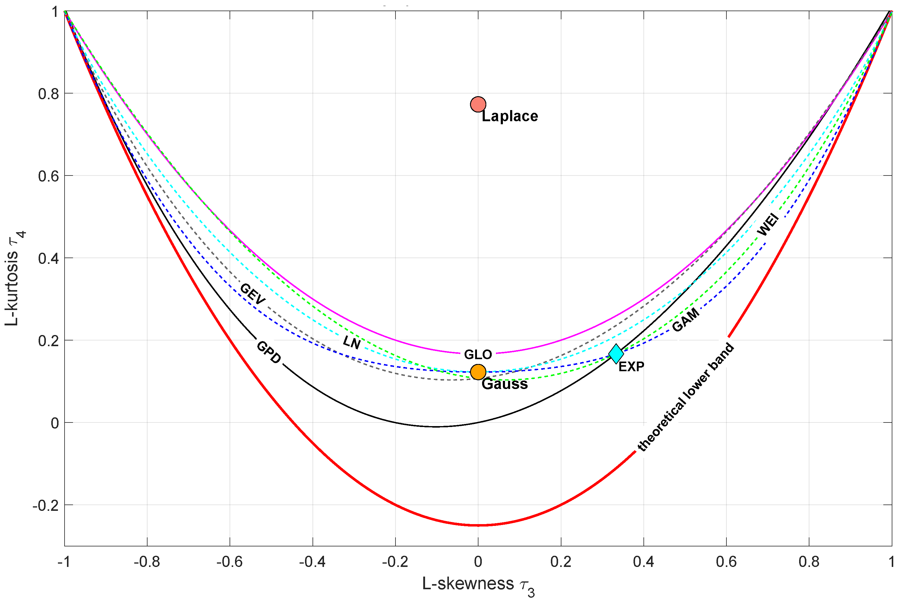
L-moments have been introduced by Hosking [18]. The LMRDs are popular in the extreme analysis. They allow the identification of proper distribution for empirical observations. The LMRD() is the most common and it shows the L-kurtosis versus L-skewness . Similarly to MRDs, one can confront the empirical data with the theoretical PDF candidate [19]. A blank diagram with shapes (points or curves) for some theoretical PDFs is presented in Figure 1.
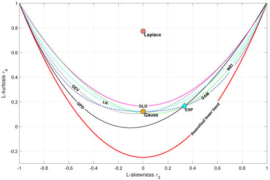
Figure 1.
Sample LMRD() diagram—red line depicts the limit of all distributions (GEV—Generalized Extreme Value, GAM—Gamma, WEI—Weibull, GLO—Generalized Logistic, GPD—Generalized Paerto, LN—Lognormal).
Similarly to the MRD(), there are two LMRD versions: LMRD() and LMRD(). They combine in a single plot the scale and skewness. As the CPA analyzes frequently use kurtosis, it is proposed to investigate a new formulation: the LMRD(). The LMRDs are the successor of the MRDs and predecessor of the IRDs and they should be considered from that perspective.
3.7. The -Stable Distribution
Apart from the specific robust estimators or L-moments one may use other distributions. Stable functions deliver an alternative set of the statistical measures [28]. The -stable distribution is expressed by the characteristics equation
where
The factor is called the index of stability (stability exponent), the is the skewness factor, the shift and the scale. Thus, the -stable distribution has one shift factor, one scale and two shape coefficients: and .
The -stable distribution has an increasing potential in the assessment approaches [29], as it allows to measure the data diversity (scale factor ) and other shaping factors such as skewness () and the tailedness (). These features nominate them as the potential measures in the residual analysis as well. Their application might be constrained in case of data, which does not fall into the stable families, which should be validated before their use.
3.8. Tail Index
Statistics frequently use the law of large numbers and the central limit theorem. Once data exhibits outliers, which is revealed in the form of tails, the majority of the assumptions made are not met. In such a case the knowledge of where the tail starts and which observations are located in the tail plays an important role [30,31]. There are many methods to estimate it and the tail index, denoted as , is the most promising one [32]. There are quite a few tail index estimation approaches, with two leading ones: the Hill [33] and Huisman estimator [34]. This work uses the second one.
Tail index as such is an extension of the -stable distribution’s stability exponent and it measures where the distribution tail starts. This perspective nominates the tail index as the potential measure of the data properties and their contamination with anomalies.
3.9. ARFIMA Models and Fractional Order
The ARFIMA time series is treated as an extension to the classical ARIMA regression models, see [35]. The process is denoted as ARFIMA
where and are polynomials in the discrete time delay operator , is random noise with finite or infinite variance. We use Gaussian noise in this research. Fractional order refers to process memory.
For the process exhibits long memory or long-range positive dependence (persistence). The process has intermediate memory (anti-persistence) or long-range negative dependence, when . The process has short memory for ; it is stationary and invertible ARMA. ARFIMA time series is calculated by d-fractional integrating of a classical ARMA process. The d-fractional integrating through the operator causes the dependence between observations, even as they are far apart in time.
The Geweke–Porter–Hudak (GPH) estimator proposed by [36] uses a semi-parametric procedure to estimate the memory parameter for ARFIMA process :
Next, ordinary least squares (LS) are applied to estimate from the
being evaluated for fundamental frequencies , , , where m is the largest integer in and is a constant. Discrete Fourier transform is evaluated as
Application of the least squares algorithm to the Equation (16) yields to the final formulation
where being a periodogram and . The GPH algorithm calculates the without explicit assumptions about ARMA polynomial orders. We use the [37] implementation.
The use of the Geweke–Porter–Hudak fractional order estimation in the assessment task is relatively new [38] and still requires much attention. Nonetheless, the first results are quite promising and that is why they are included in the analysis. However, the argumentation could be extended to the fractal, multi-fractal and data persistence time series assessment perspective of this estimator, which finds earlier references [39,40].
4. Estimation Approaches
This section describes the machine learning approaches taken into account during the study. We decided to apply only black-box identification approaches [41]. This choice is motivated by the unknown patterns behind the data due to the dynamic geopolitical situation in recent years and due to the specificity of market practice during the determination of the price for very short shipping. Among other factors, rising inflation, Brexit and the COVID-19 pandemic are impacting truck cargo transit prices. Proposing an explicit form of the cost model that takes into account the aforementioned factors would have been a difficult task, which we decided not to undertake.
4.1. Classical Regression Models
The following regression estimation algorithms are used during the analysis.
4.1.1. Linear Models
Linear regression, like the least mean squares (LMS), is frequently the natural first choice. LMS minimizes the sum of the squares of the differences between the actual and the estimated value (model residuum). LMS is the simplest regression approach, however it is highly sensitive to outliers [42]. Robust Linear Regression [43] (R-LMS) with the intercept and linear terms compared to LMS is affected by outliers only in a minimal scale. Stepwise Linear Regression [44] (SLR) is a method that reduces the influence of less important parameters in an iterative way.
Outliers were expected to occur in the dataset, such as single long-distance transports. Regression models robust to multivariate outliers, namely Theil-Sen [45] (TS-LR) and Huber [42] regressors (H-LR), are also tested. Huber regressor differs from the Theil-Sen one, because it does not ignore the effect of the outliers, giving just a smaller weight to them.
4.1.2. Support Vector Machine
Due to the existence of many transport parameters, it was problematic to divide the data into separate sets to infer the costs of new transports. For this purpose, it was reasonable to use hyperplane methods such as Support Vector Machines [46]. Using this method, we are able to approximate the costs of new transports by reference to a test set divided into sets with a predetermined precision. In this method, we can adjust the parameters to achieve a balance between the generalization of the model and its sensitivity.
Linear Support Vector Machines [47] (LSVM) is the simplest linear kernel (20) version of the method. It is particularly effective when dealing with linear relationships between input features and the target variable. Its aim is to identify the optimal hyperplane, minimizing the error between the predicted values and the actual results. Its biggest advantages are simplicity, efficiency and robustness to outliers, but it is ineffective when dealing with complex, non-linear relationships.
Quadratic Support Vector Machine [48] (QSVM) is an extension of the LSVM. Unlike the linear version, it uses a quadratic kernel function (21) that allows the capture of more complex decision constraints. It can be particularly useful when dealing with datasets where classes are not linearly separable.
Coarse Gaussian Support Vector Machine [49] (CGSVM) is suited to tasks with low-complexity data. It uses Coarse Gaussian kernel that is given by the Formula (22)
Medium Gaussian Support Vector Machines [49] (MGSVM) is mainly suited to tasks with medium-complexity data. It uses Medium Gaussian kernel that is given by the Formula (23)
Following, the Fine Gaussian Support Vector Machines (LGSVM) use the Formula (24)
Kernel Support Vector Machine [50] (KSVM) belongs to the group of kernel approximation models. Using this method, we can conduct nonlinear regression on large datasets. Training and prediction processes will generally run faster for this method than for Gaussian kernel SVM models. Metric used in model fitting is epsilon-insensitive loss.
4.1.3. Gaussian Processes
The dataset that we use is not particularly large. We search for a regression model that handles data sets of small size reasonably well. In such a case the use of Gaussian Process Regression [51] is justified, because it allows us to determine the uncertainty of the transportation cost prediction as well. Gaussian Process Regression is a non-parametric approach, which is based on kernel probabilistic models.
Exponential Gaussian Process [52] (EGPR) uses exponential kernel, which is stationary kernel and can be parameterized by a length scale. Kernel is given as a fraction of Euclidean distance and length scale parameter. By taking to the kernel squared value of Euclidean distance we will obtain Squared Exponential Gaussian Process (also named radial basis function kernel [53]—SEGPR). The advantage to this development is the small chance of generating large errors, while handling extensive data sets in higher dimensions. Matern Gaussian Process Regression (MGPR) is the next extension to the Gaussian algorithm and is generalization of radial basis function kernel. The Matern kernel uses spectral densities of the stationary kernel and create Fourier transforms of the RBF kernel. Rational Quadratic Gaussian Process Regression [54] is a probabilistic method that is effective when dealing with non-linear relationships. The model defines a distribution over possible functions of the relationship between the input features and the target variable. In this method, the kernel is used to capture the similarity between data points, allowing the model to make predictions based on relationships of points in the training data. The Rational Quadratic kernel enables the model to capture a broader range of non-linear patterns in the data.
4.1.4. Nearest Neighbors
In order to check whether better results would not be achieved by averaging the known costs of several similar transports, the k-nearest neighbors method was used. The k Nearest Neighbors method (k-NN) [55] is based on searching the training set to find transports with parameters closest to the one whose cost we are looking for. This method uses ”k” such known transports.
This algorithm is sensitive to local structures of data due to using set of transports with the most similar parameters, but is not prone to outliers from the training set [56].
4.1.5. Orthogonal Matching Pursuit
Orthogonal Matching Pursuit (OMP) stands as an algorithm in compressing sensing, adept at recovering sparse signals within noisy linear regression models [57]. This technique enriches the foundational Matching Pursuit algorithm through a least-squares minimization at each step, thereby optimizing approximations of the extant elements. Noteworthy is the inherent restraint against redundant element selection, attributed to the orthogonal relationship between the residual and the previously chosen constituents. Consequently, the residual converges to zero after k iterations. The first publications within the domain of signal processing regarding Orthogonal Matching Pursuit appeared in 1993 [58].
4.1.6. Ridge Regression
Ridge regression (RR) addresses multicollinearity by improving least squares estimates, which suffer from bias and high variance in such scenarios [59]. By introducing controlled deviation to regression estimation, ridge regression curbs standard error and enhances reliability, albeit at the expense of some accuracy. It indirectly combats multicollinearity through a constraint length factor, relinquishing unbiasedness for more practical and robust regression coefficients. This method’s flexibility blends qualitative and quantitative analysis, offering a unique solution to multi-collinearity and finding application in extensive research. However, diverse ridge parameter calculations yield divergent results, and the popular ridge trace approach relies on subjective variable selection, posing arbitrary outcomes.
Moreover, it is noteworthy that the conventional ridge regression methodology does not inherently facilitate variable reduction, leading to the retention of all variables within the model. In response to this, the utilization of the Automatic Relevance Determination (ARD-RR) method emerges as an approach capable of decisively assessing the relevance of input features [60].
Furthermore, our approach encompasses the utilization of Bayesian Ridge Regression [61] (BRR), wherein is assumed that all regression coefficients have common variance. The Bayesian instantiation of ridge regression presents a distinct advantage by obviating the necessity for explicit regularization parameter selection. Instead, the model dynamically acquires this parameter from the data, engendering a more data-driven and adaptive regularization strategy.
4.1.7. Decision Trees
Searching for a regression method that would allow us to create an accurate and robust model, we also had non-technical aspects in mind. This was one of the reasons to use decision trees [62]. One of their many advantages is that the model is intuitive and easy to explain to the decision makers for whom the model is being developed.
Regression trees [63] are a supervised learning approach that is commonly used in statistics and data mining. They are one of the most popular algorithms in machine learning. The algorithm works by dividing the data set into subsets (branches, nodes and leaves). The division is made in such a way as to obtain the greatest possible information gain or to minimize the sum of squared errors (SSE). The unquestionable benefit of this approach is its robustness to outliers and missing data. Unfortunately, the growth of the regression tree is associated with a significant increase in computational complexity (therefore, the depth of the tree can be limited).
Regression Tree [64] (DTR) divides the data into branches, nodes and leaves. Regression Tree is similar to Decision Tree that is used to predict continuous data, not only discrete data output. Regression Tree can be classified by its size, defining the depth of the regression tree. Division is created by leaf size parameter. Coarse Regression Tree has a minimum of 20 Coarse Trees, Medium Regression Tree (M-DTR) has a minimum of 12 medium trees and Fine Regression Tree has 4 fine trees. Fine Regression Tree (F-DTR) is usually highly accurate on the training data, however separate test data accuracy can be not comparable to training one. Coarse Regression Tree (C-DTR), due to the multiplicity of leaves, is inclined to overfit data. However, Coarse Tree with limited large leaves does not gain high training accuracy and its training accuracy might be close to the test one.
Boosted Regression Trees [65] (BoostRT) are an advanced machine learning approach used for regression tasks, when there are non-linear relationships in the data. Boosting in the method consists in the iterative matching of trees to test data based on the residual error. Boosted Regression Tree has found wide applications in various domains, including finance, healthcare and environmental science, owing to its ability to handle high-dimensional data and produce accurate predictions. The disadvantage of this method is that its performance is highly dependent on careful parameter tuning and sufficient training data to avoid overfitting.
Gradient boosting stands as a prevalent and effective machine learning technique, extensively applied to regression and classification tasks. The development of gradient boosting can be attributed to the work of Jerome H. Friedman [66]. This methodology culminates in the formation of an ultimate predictive model structured as an ensemble amalgamating numerous feeble predictors. At its core, gradient boosting is a process of iteratively refining a cost function within the expanse of function space. This iterative refinement is achieved by judiciously selecting functions that align with the negative gradient orientation of the cost function. Often, the ensemble constituents of gradient boosting harness decision trees as weak predictors. The amalgamation of decision trees and boosting principles results in the Gradient Boosted Decision Tree. In the Gradient Boosted Decision Tree paradigm (GBoostRT), an iterative construction unfolds, progressively assembling an ensemble of modest decision tree learners through the mechanism of boosting. The culminating prediction yielded by Gradient Boosted Decision Tree is the aggregate outcome of assimilating the prediction outputs from all constituent trees, thereby harnessing the collective predictive prowess of the ensemble.
Histogram-based Gradient Boosting Regression Tree (HGBoostRT) represents an estimator endowed with capabilities to handle missing values (NaNs) [67]. Throughout the training process, the growth of trees entails a learning mechanism that strategically determines the trajectory of samples with missing values, directing them to either the left or right child nodes, predicated upon the ensuing potential gain. During prediction, samples harboring missing values are systematically assigned to the appropriate child node. In instances where a specific feature encountered no missing values during the training phase, samples replete with missing values are routed to the child node boasting the highest sample abundance. This estimator exhibits significantly heightened efficiency compared to the Gradient Boosting Regression tree, particularly in the context of substantial datasets.
Extremely Randomized Trees Regression [68] (ERTR) is a similar but significantly faster variant of random forests method. This algorithm creates numerous decision trees and predictions are made by averaging the prediction of the decision trees. Each tree is built based on a randomly chosen subset from the feature set. Splitting value is also chosen randomly—we do not calculate entropy, information gain or SSE error as in classical regression trees. This allows us to reduce the correlation of individual trees. The main advantages of this method include improved prediction accuracy, overfitting control and reduction in bias.
Bagged Regression Trees Regression [69] (BRTR) is a supervised machine learning algorithm. The main idea of Bagged Trees is to not rely on a single decision tree, but be dependent on many decision tree models. It is used to increase predictive power and stability of regression trees. The main advantage of using Bagged Trees is its ability to minimize variation while holding bias consistent. In general, decision trees are simple and easy to explain,; however, bagged trees algorithms append complexity, so they can be difficult to interpret.
4.1.8. Random Forest Regression
A decision forest in the Random Forest Regression (RFR) can be defined as an ensemble classifier comprised of an amalgamation of tree-structured classifiers. Each individual tree within this ensemble contributes a singular vote towards the prevailing class of the input data point. Remarkable enhancements in classification accuracy have been consistently noted, irrespective of the specific algorithms employed for the construction of the constituent trees [70].
4.1.9. Regularization Techniques
Equally important as the predicted shipping cost are the features/information based on which this cost was calculated. During preprocessing, you can a priori select the features based on which you build the model, but you can also use the LASSO [71] regression (LASSO-R) model to select these features. LASSO (least absolute shrinkage and selection operator) method reduces model overfitting by extending the cost function with a penalty term i.e., the sum of the L1 norms of the model coefficients. By minimizing the value of the cost function, the method identifies features that are irrelevant from its point of view. Using this model, the transport company will know which transport parameters it can afford to deviate from the norm without changing the cost of shipping.
A commonly used alternative to the LASSO model is the LARS model [72]. It is used for multidimensional data—such as the data from the shipping company on which our experiments are being conducted. In the case of LARS (least-angle regression) method, there is no need to adjust the hyper-parameters weighing the penalty term. LARS is quite similar to forward stepwise regression method. The Least Angle Regression method aims to find an attribute that has the highest correlation with the residual. However, despite the high numerical efficiency of this method, it is very sensitive to noise, which can lead to misleading predictions and, consequently, financial losses for the company that uses such a model.
The concept of a regressor combining the advantages of the above two has also emerged. Such model is LARS LASSO (LARS-R). It has a faster convergence than the standard LASSO method. This method has also only two hyper-parameters, so tuning the model is greatly simplified.
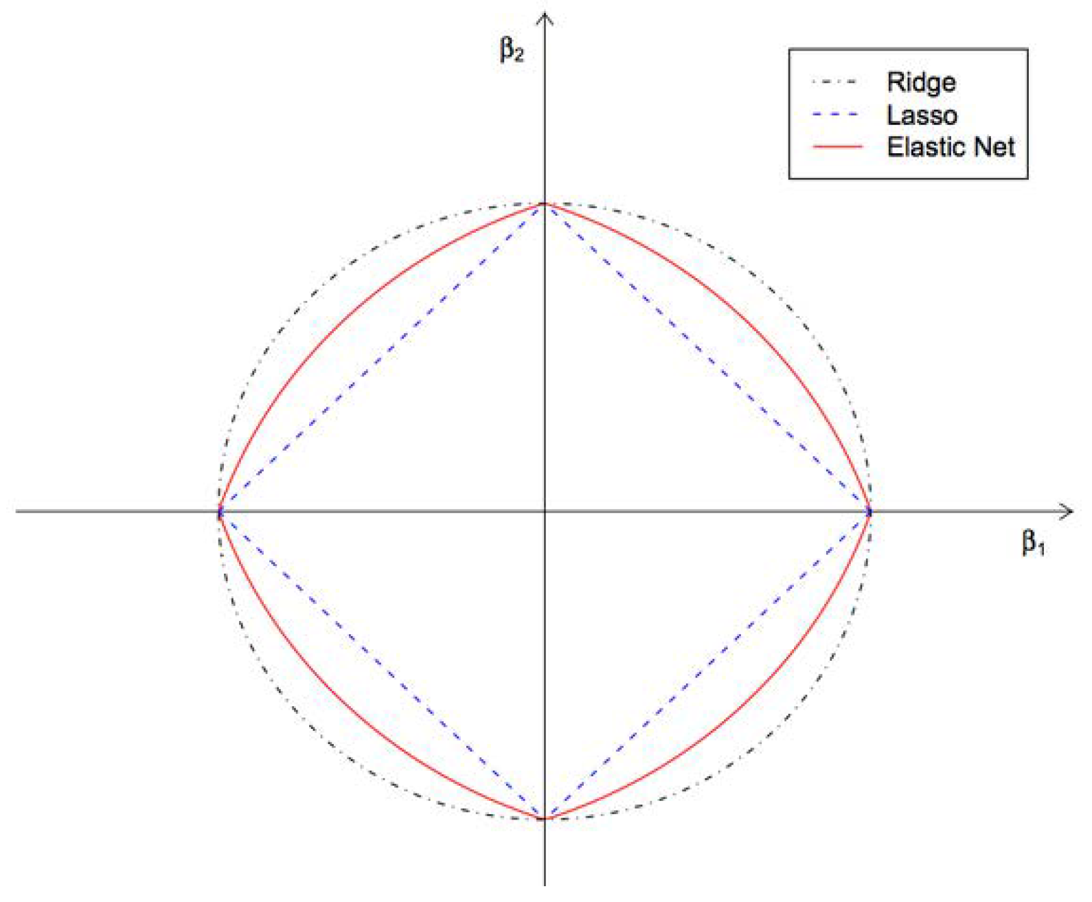
Another example of a hybrid method that combines the advantages of other methods (LASSO and Ridge) is the Elastic Net method [73] (ENR). It handles multi-collinearity issues extremely well. The penalty function incorporates both L1 and L2 norms (see Figure 2). It reduces overfitting by eliminating redundant (mutually correlated) features.
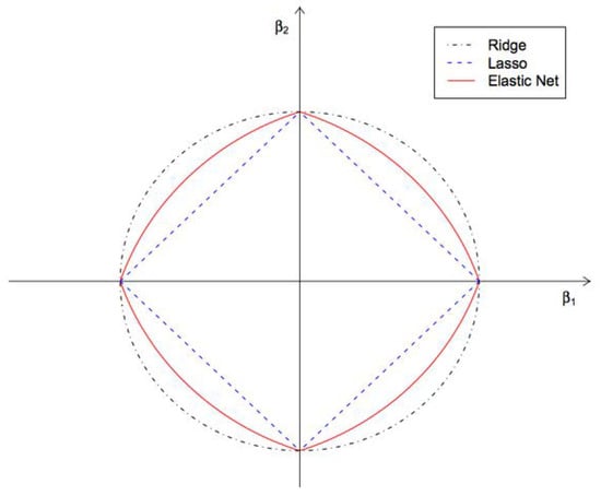
Figure 2.
Norms used for regularization in Ridge, LASSO and Elastic Net regression methods.
4.2. Neural Network Approach
In order to develop transport cost prediction models, it was decided to use the PyTorch library, which allows numerical calculations, including operations on tensors and the implementation of advanced neural networks. The problem is the lack of knowledge of the ideal neural network architecture that would handle this task the best. Therefore, a study was conducted, exploring various possibilities, such as the number of hidden layers, the number of neurons in each hidden layer, the activation functions and the network training process optimizer. Details of the architectures used are as follows:
- Number of hidden neurons: 12–2048;
- Number of hidden layers: 1–8;
- Activation fun.: RELu, Tanh, identity, logistic;
- Optimizer: Adaptive Moment Estimation, Stochastic Gradient Descent.
The use of artificial neural networks (ANN) in the context of cost prediction problems has found application in a number of scientific studies on such topics as predicting the cost and duration of building construction or predicting the cost of housing engineering [74,75].
5. The Results
We start the analysis with a presentation of the calculation of common integral measures. Table 4 compares obtained values. Even the draft analysis allows for an interesting observation. Each measure indicates different models as the best. The MSE highly penalizes large errors [76] and is sensitive to any outlying occurrences, while the MAE is less conservative. It enables closer relations to smaller variations and economic considerations [77].

Table 4.
Comparison of the regression models. Grey color highlights the extreme values of the models: the worst (red) and the best (green). Bold numbers indicate the worst and the best one.
Moreover, relative indexes point out or penalize other methods. Therefore, the decisions about the model that should be chosen highly depends on the selected index. Practice shows that this decision is often unaware, which might be costly in further practical applications.
In Section 3, we describe various performance indexes that can be found in the literature. Moreover, we suggest the performance of visual multi-criteria analysis using the so-called Index ratio Diagrams (IRD). This idea follows the notions of moment ratio diagrams, known in statistics.
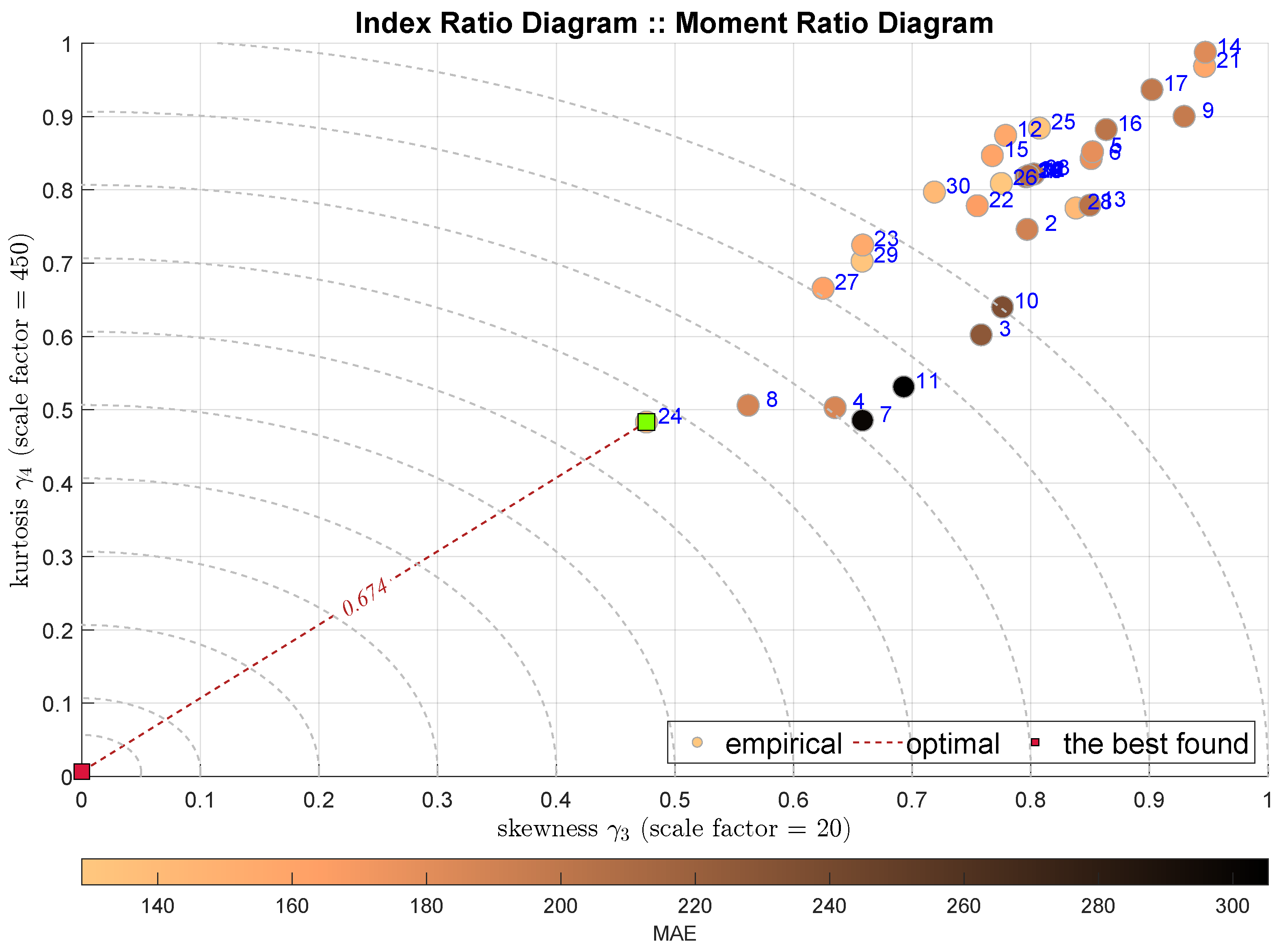
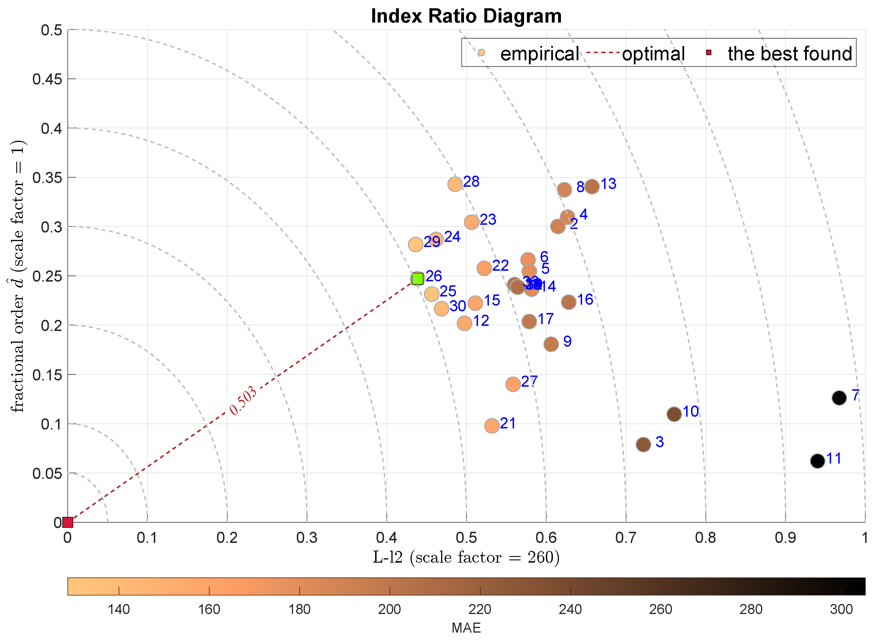
We start the analysis from the classical moment ratio diagram that shows the relationship between the third and the fourth moment, i.e., between the skewness denoted as and the kurtosis . Figure 3 presents the respective diagram. Each shaded circle denotes one model, which is labeled with the blue number according to the notation sketched in Table 4. The circles are shaded according to some other index, in this case it is the MAE. Generally, such a drawing brings some relative visual information—we still expect to obtain a single performance indicator. Actually, we may assume that the best tuning is reflected by the shortest distance from some optimal point. In this case we may assume the point .
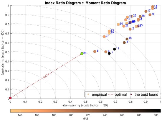
Figure 3.
IRD(,): red square depicts good tuning, green—the best (circles shaded according to MAE).
As we wish to obtain this value independently, we scale it and obtain the following IRD distance index dIRD(x,y) for scaled values x and y:
This index we name as the Aggregated Distance Measure (ADiMe). The assumed scaling factors, which are used in each case, are denoted on the plots.
The IRD(,) diagram points out the model no 24, i.e., the Histogram Gradient Boosting Regression (HGBoostRT) as the best modeling approach. We may observe that selected model is the same as the one selected by the MSE index. The value of the IRD distance index is equal to 0.674. What is interesting is that the second-best model is the Quadratic Support Vector Machine (QSVM), which is not appreciated by any of the integral indexes.
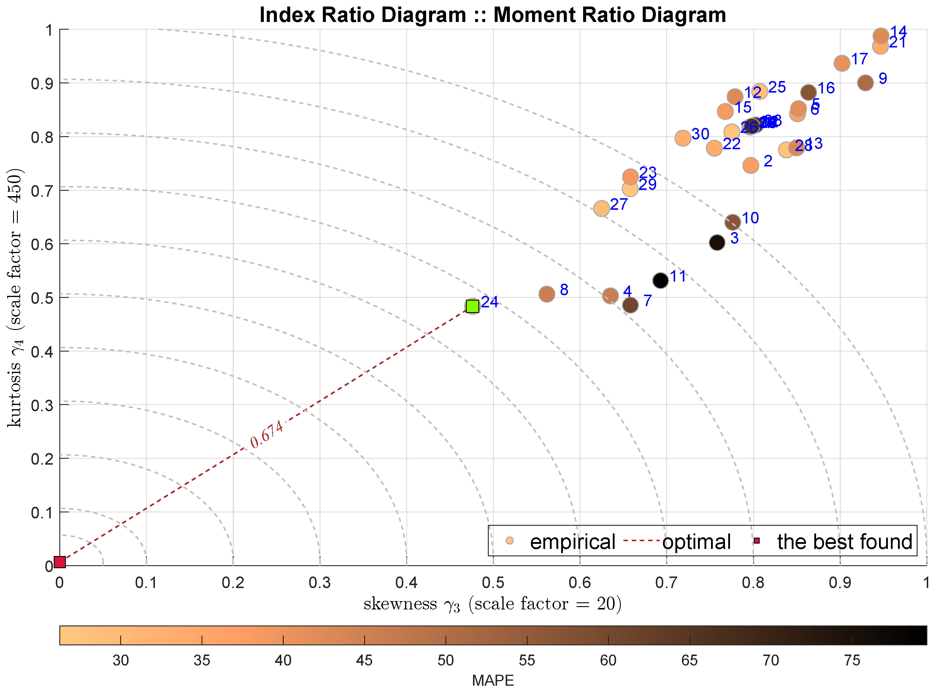
The next Figure 4 presents the same IRD relationship IRD(,), but with different shading, which is conducted according to the relative MAPE index. It is decided that all the consecutive diagrams are shaded according to the MAE index.
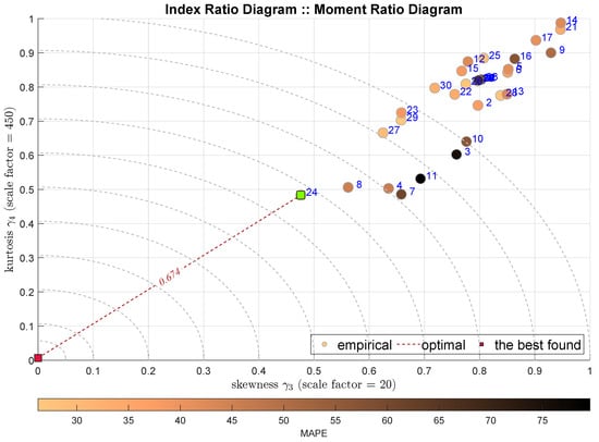
Figure 4.
IRD(,): red square depicts good tuning, green—the best (circles shaded according to MAE).
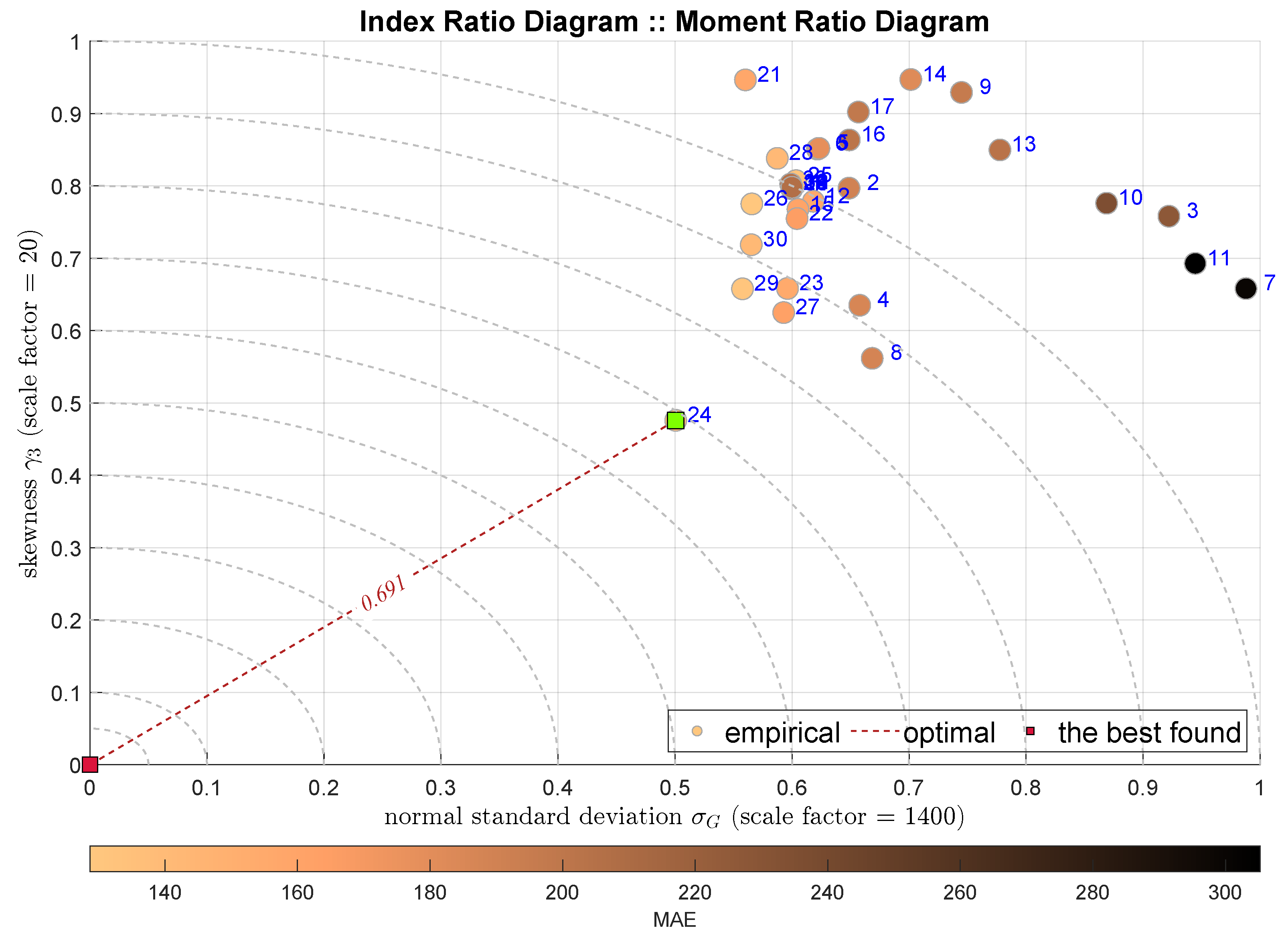
The next two plots show the IRD diagrams showing the relationship between the standard deviation (the second moments) and the skewness. Figure 5 uses classical Gaussian standard deviation estimator , while Figure 6 uses its robust counterpart . In both cases the HGBoostRT model is indicated with the ADiMe measure equal to and . In contrast, the next-best models are different, i.e., the Fine Regression Tree (F-DTR) and Coarse Regression Tree (C-DTR).
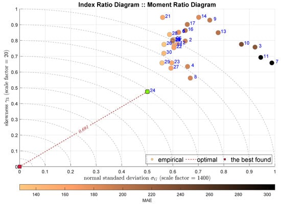
Figure 5.
IRD(,): red square depicts good tuning, green—the best (circles shaded according to MAE).
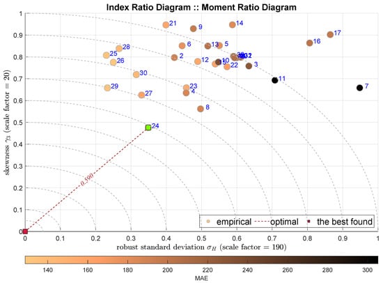
Figure 6.
IRD(,): red square depicts good tuning, green—the best (circles shaded according to MAE).
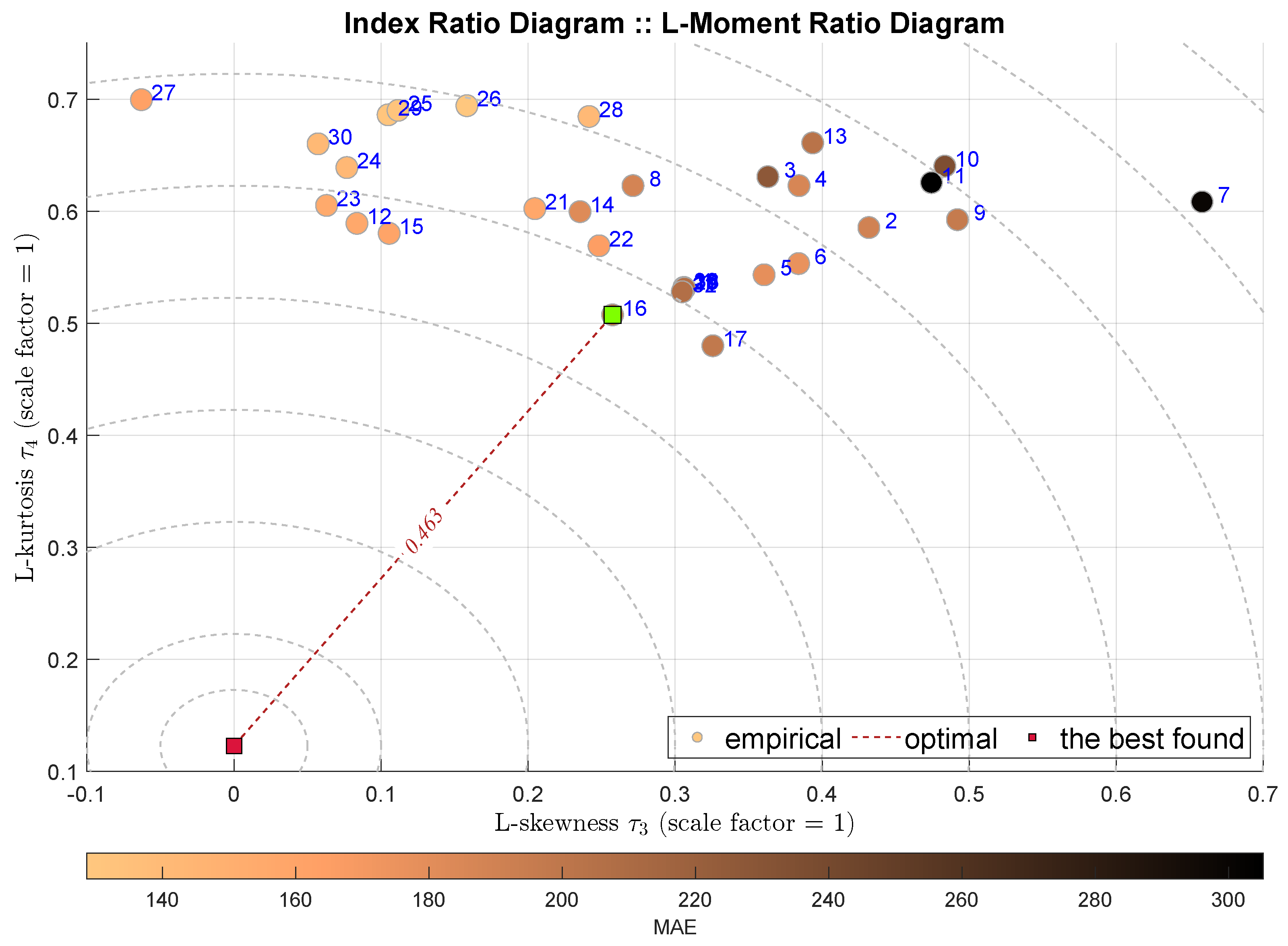
Figure 7 presents standard L-Moment Ratio Diagram, i.e., the IRD(,). As the L-skewness and L-kurtosis are normalized, there is no need for any further scaling. This approach indicates the k-Nearest Neighbors Regressor (k-NN) with . Interestingly, the two next-best models are Rational Quadratic Gaussian Process Regression (RGPR) and Exponential Gaussian Process Regression (EGPR). The favoring of these models is intriguing, because they are not indicated by other indicators. We may bring the hypothesis that their residua exhibit, in general, neutral statistical properties. This issue requires further investigation.
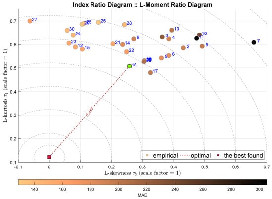
Figure 7.
IRD(,): red square depicts good tuning, green—the best (circles shaded according to MAE).
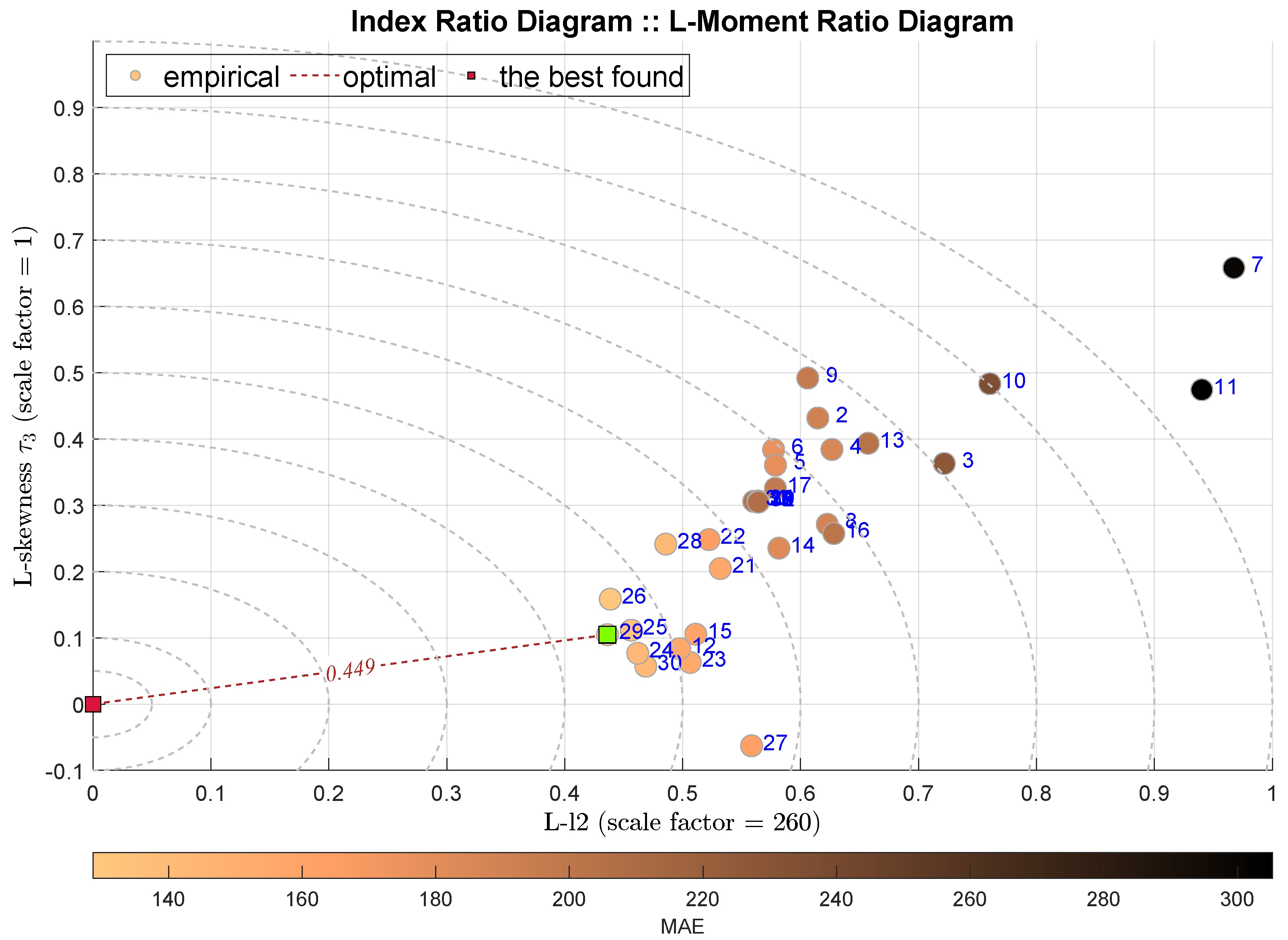
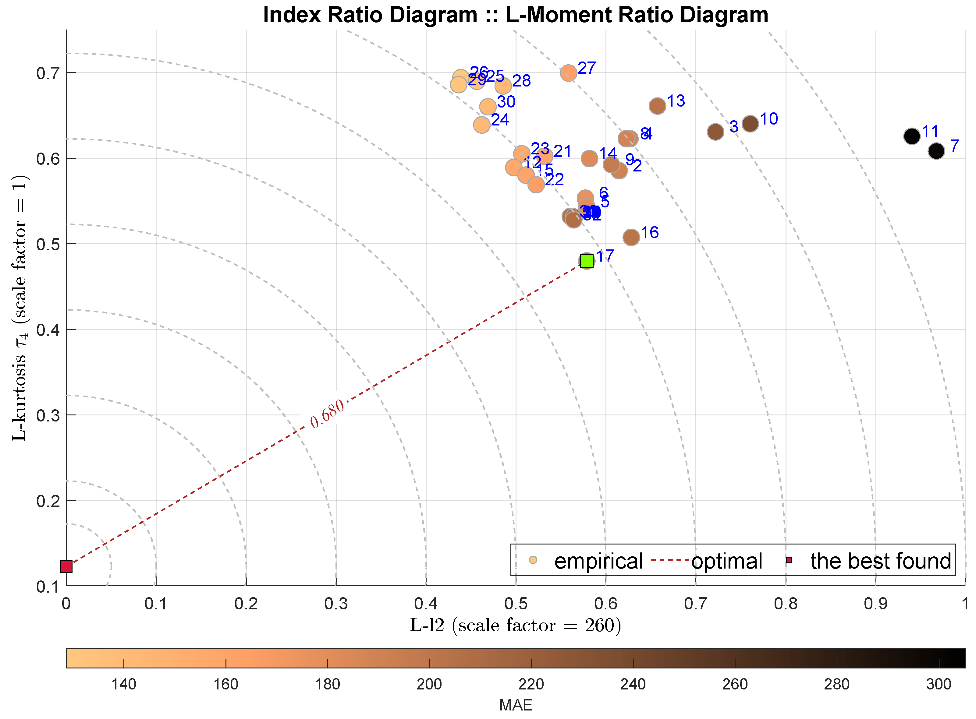
The following two diagrams takes into account the L-l2 scale measure together with the L-skewness in Figure 8 and L-kurtosis in Figure 9. The IRD(L-,) approach points out the Coarse Regression Tree (C-DTR) with , which is highly favored by all integral measures. On the contrary, the IRD(L-,) selects the Orthogonal Matching Pursuit (OMP) method with . It must be noted that the selected best models are quite close to the following ones, and thus the indications are not very decisive.
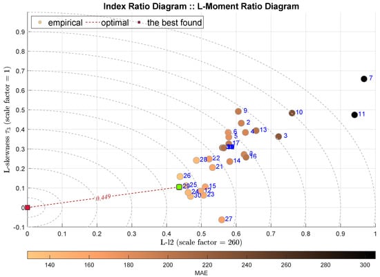
Figure 8.
IRD(L-,): red square depicts good tuning, green—the best (circles shaded according to MAE).
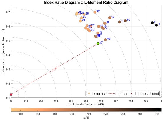
Figure 9.
IRD(L-,): red square depicts good tuning, green—the best (circles shaded according to MAE).
The next two plots combine the L-scale factor L-l2 with the alternative measures of the tail—the tail index in Figure 10 and the Geweke–Porter–Hudak ARFIMA filter fractional order estimator shown in Figure 11. Both diagrams select the same modeling approach, the Bagged Regression Trees (BRTR), which is highly favored by the MAE index. The ADiMe values for both approaches are and , respectively. In both cases, the second-best model is Extremely Randomized Trees (ERTR).
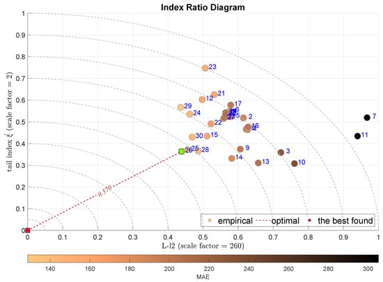
Figure 10.
IRD(L-,): red square depicts good tuning, green—the best (circles shaded according to MAE).
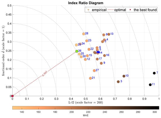
Figure 11.
IRD(L-,): red square depicts good tuning, green—the best (circles shaded according to MAE).
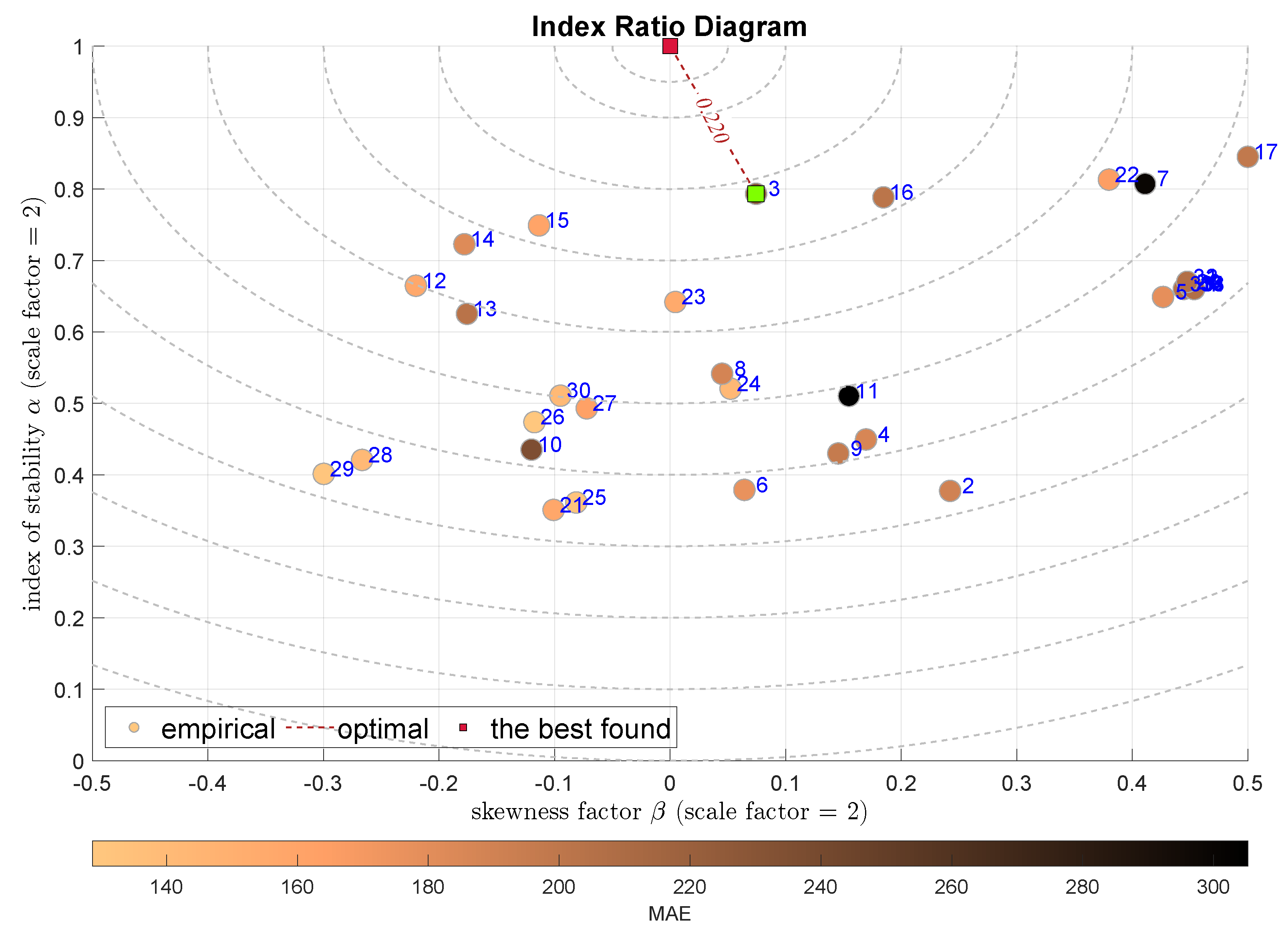
Finally, the IRD diagrams are constructed using factors of the -stable distribution. Figure 12 presents the model selection according to the combination of the skewness and the stability exponent . The considered optimal point is the , where this point indicates normal distribution. In that sense, the Stepwise Linear Regression model (SLR) is selected with the . The next-best models are the RGPR—Rational Quadratic Gaussian Process Regression—and the k-NN.
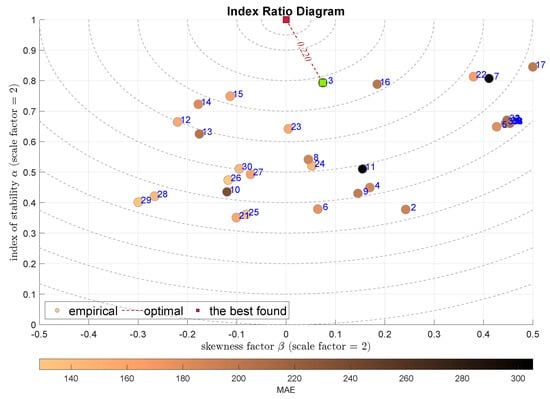
Figure 12.
IRD(,): red square depicts good tuning, green—the best (circles shaded according to MAE).
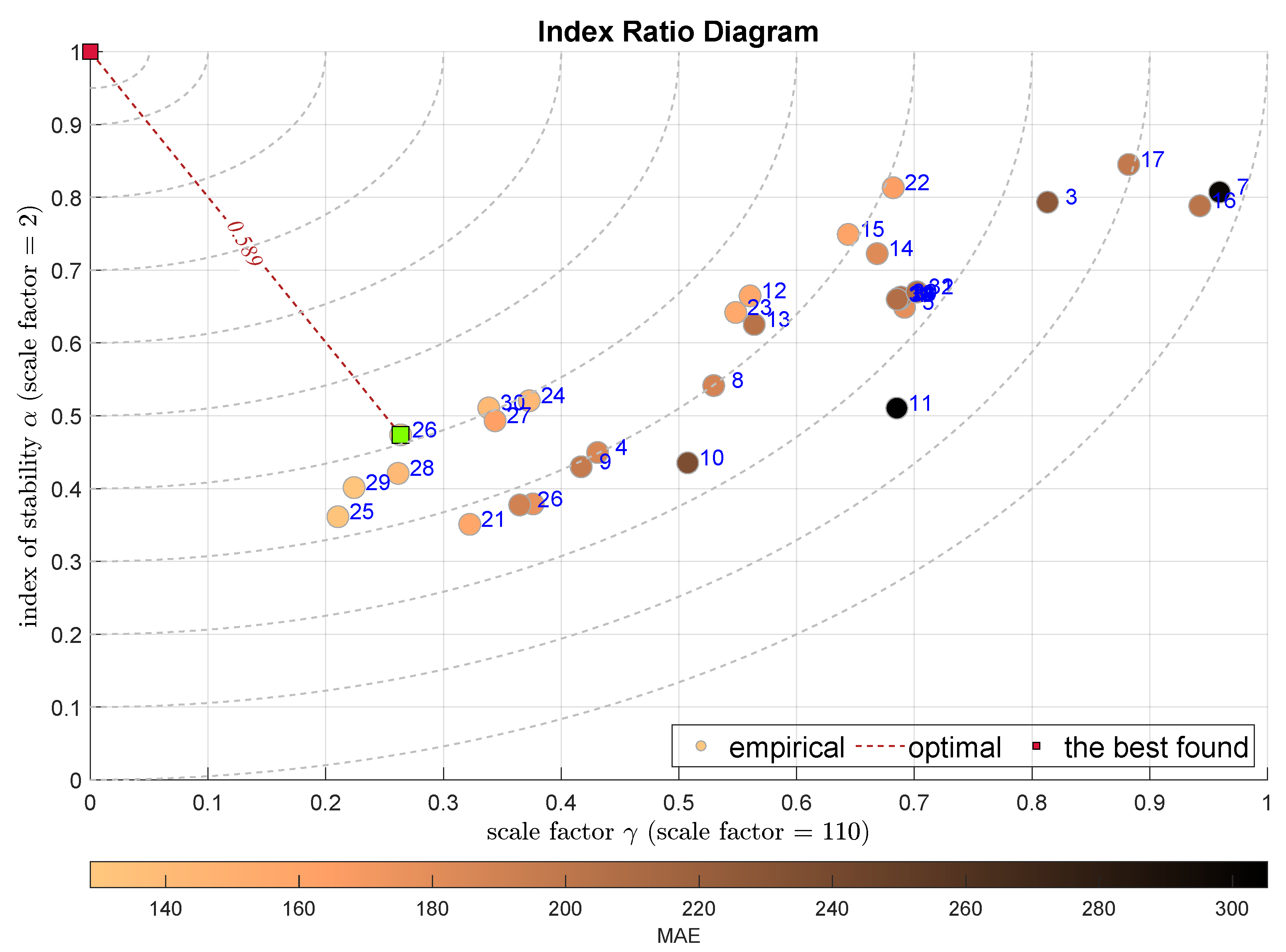
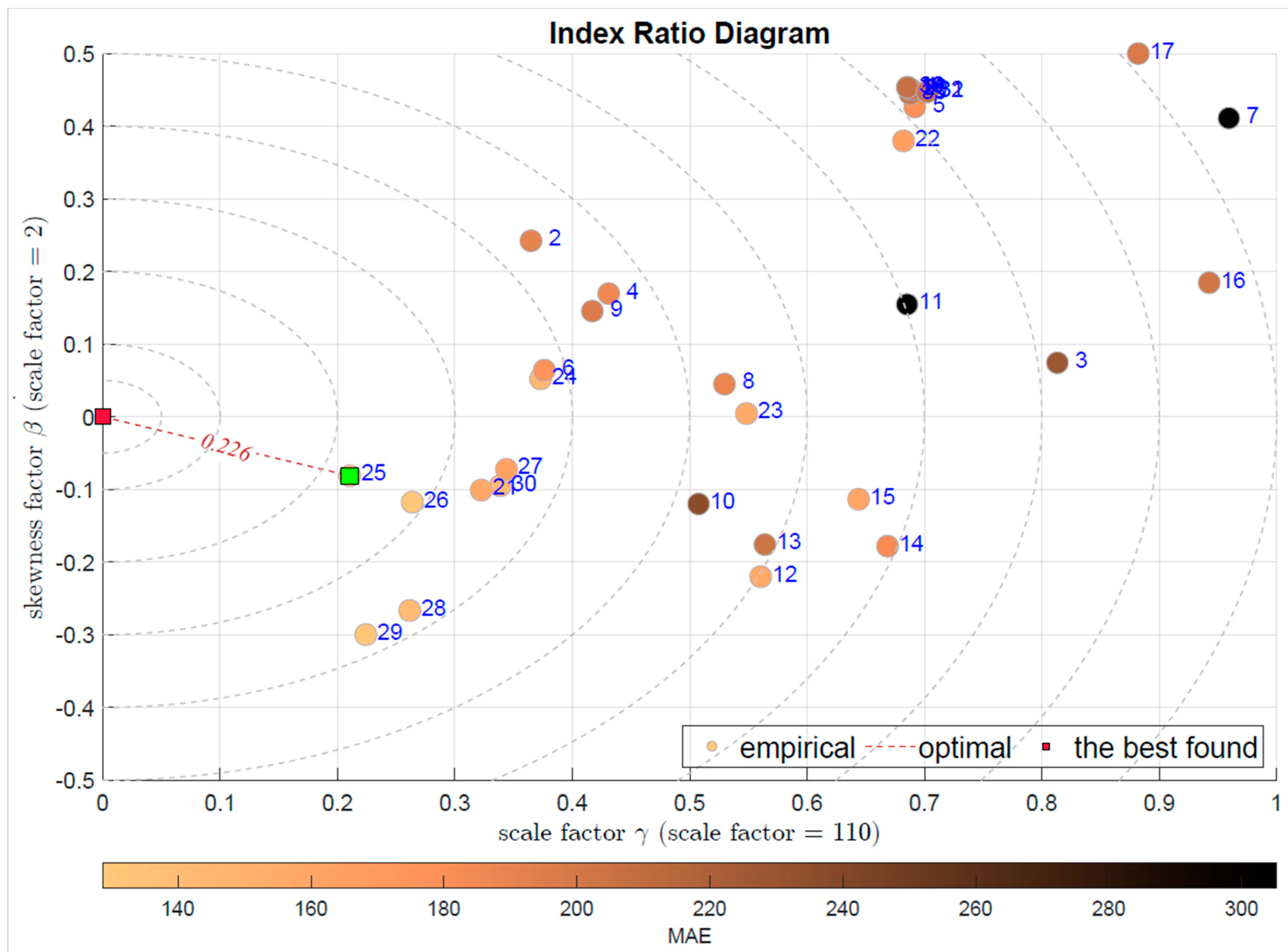
The last two plots present the combination of the scale factor together with stability exponent in Figure 13 and with the skewness in Figure 14. The first one selects the Bagged Regression Trees (BRTR) approach (), while the latter the Extremely Randomized Trees (ERTR)—. Both modeling approaches are seriously favored by the integral indexes.
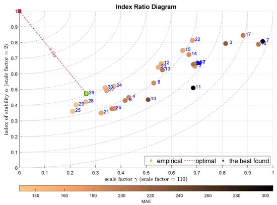
Figure 13.
IRD(,): red square depicts good tuning, green—the best (circles shaded according to MAE).

Figure 14.
IRD(,): red square depicts good tuning, green—the best (circles shaded according to MAE).
It should be noted that the difference between these two diagrams is quite significant. The shape factor is responsible for the tails, i.e., informs about the ratio of the outlying observations, while the second shape factor, the skewness measures the residuum asymmetry. With this difference kept in mind we may select which feature of the modeling error is considered to be the most important for us.
Finally, let us compare all the approaches and the features they favor and the models they indicate. Table 5 aggregates the features favored by each of the IRD diagrams with the selected model.

Table 5.
Comparison of the ADiMe indications.
Generally, the regression trees approaches are the best fitted to the considered estimation task. However, each method has different features and objective comparison is highly relative and sensitive to the selection of the index. The Histogram Gradient Boosting Regression method captures the outliers and utilizes them in the estimation, while the k-NN approach focuses on the bulk of the data and neglects the outliers.
Concluding, one should first define which feature of the estimations matters the most, and according to that one should select the assessment methodology and the indexes used. The scaling indexes and the visual inspection of the IRD diagrams deliver an additional degree of freedom, allowing for deeper insight into the properties of the considered model.
6. Conclusions and Further Research
This works focuses on two aspects. It addresses the issue of the cost estimation for the short routes of the external FTL fleet. This subject is hardly recognized in the literature, it is really difficult and has large practical importance.
The second contribution, in our opinion the most important, is connected with the model assessment. It is very subjective to assess the model, as we do not have a single universal measure. Each index favors different properties. If we neglect that fact, the resulting model can miss our expectations without any clue why. The model assessment should not be limited to the simple comparison of a single measure numbers, but deeper investigation and appropriate index selection, even using visual inspection, might help. We propose to use the novel approach using Index Ratio Diagrams (IRD) and resulting Aggregated Distance Measure (ADiMe).
The practical perspective of this research has three dimensions. It bridges the gap between statistics and machine learning, as nowadays researchers tend to forget the potential lying in statistical analysis. The review of the ML-based estimation reports and papers does not deliver positive conclusions. Almost always, authors do not try to assess why their model is so good or so bad. They simply report residuum measure index, often using one single value. They do not try to check whether their selection captures data properties. This work aims to show that the assessment task is not one-dimensional and the analysis of the nuances can improve the work and the knowledge. This fact has further and more significant consequences. Obtained models might be not so good as observed, and therefore the industrial end-user can be frustrated by the results. That might lead to a lack of satisfaction, no further use of the tool and general robustness to new ideas.
Finally, this work offers the method of multicriteria residual analysis accompanied with new, almost unknown measuring opportunities that can highlight currently unobserved properties.
The proposed method is not universal and some limitations might be observed. First of all, especially at the level of the results presentation to the end-user, it might be challenging to explain the conclusions. Also, the selection of the scaling index values might be subjective and the work on the results normalization is still required. It would be interesting to conduct more research aimed at the synthesis of the observation in the direction of the Pareto-front analysis. The connection between the IRD observations, their explanation and the way to improve the model should be investigated.
The analysis is still not over. The model assessment, though considered simple, is not as simple as perceived. One index is not equal to another index. This mistake can lead to costly consequences. A lot of subjects remain open. How can we assess models using various criteria? How can we combine our expectations about the model features with proper performance index selection? How can we make the residuum analysis simple, clear and comparable?
Author Contributions
Conceptualization, P.D.D.; methodology, P.D.D.; software, J.K., J.O., M.G. and K.B.; validation, P.D.D.; formal analysis, J.K., J.O., M.G. and K.B.; investigation, J.K., J.O., M.G. and K.B.; data curation, S.C.; writing—original draft preparation, J.K., J.O., M.G., K.B. and P.D.D.; writing—review and editing, J.K., J.O., M.G., K.B., S.C. and P.D.D.; supervision, P.D.D. All authors have read and agreed to the published version of the manuscript.
Funding
This work was supported by the Polish National Centre for Research and Development, grant no. POIR.01.01.01-00-2050/20, application track 6/1.1.1/2020—2nd round.
Data Availability Statement
The data presented in this study are available on request from the corresponding author.
Conflicts of Interest
Authors Szymon Cyperski and Paweł D. Domański were employed by the company Control System Software Sp. z o.o. The remaining authors declare that the research was conducted in the absence of any commercial or financial relationships that could be construed as a potential conflict of interest.
Abbreviations
The following abbreviations are used in this manuscript:
| LMRD | L-Moment Ratio Diagram |
| MRD | Moment Ratio Diagram |
| Probability Density Function |
References
- Morrison, G.; Emil, E.; Canipe, H.; Burnham, A. Guide to Calculating Ownership and Operating Costs of Department of Transportation Vehicles and Equipment: An Accounting Perspective; The National Academies Press: Washington, DC, USA, 2020. [Google Scholar]
- Vu, Q.H.; Cen, L.; Ruta, D.; Liu, M. Key Factors to Consider when Predicting the Costs of Forwarding Contracts. In Proceedings of the 2022 17th Conference on Computer Science and Intelligence Systems (FedCSIS), Sofia, Bulgaria, 4–7 September 2022; pp. 447–450. [Google Scholar]
- Miller, J.W.; Scott, A.; Williams, B.D. Pricing Dynamics in the Truckload Sector: The Moderating Role of the Electronic Logging Device Mandate. J. Bus. Logist. 2021, 42, 388–405. [Google Scholar] [CrossRef]
- Acocella, A.; Caplice, C.; Sheffi, Y. The end of ’set it and forget it’ pricing? Opportunities for market-based freight contracts. arXiv 2022, arXiv:2202.02367. [Google Scholar]
- Stasiński, K. A Literature Review on Dynamic Pricing—State of Current Research and New Directions. In Advances in Computational Collective Intelligence; Hernes, M., Wojtkiewicz, K., Szczerbicki, E., Eds.; Springer: Cham, Switzerland, 2020; pp. 465–477. [Google Scholar]
- Freightfinders GmbH. Freight Cost Calculator. 2023. Available online: https://freightfinders.com/calculating-transport-costs/ (accessed on 26 May 2023).
- Tsolaki, K.; Vafeiadis, T.; Nizamis, A.; Ioannidis, D.; Tzovaras, D. Utilizing machine learning on freight transportation and logistics applications: A review. ICT Express 2022, 9, 284–295. [Google Scholar] [CrossRef]
- Pioroński, S.; Górecki, T. Using gradient boosting trees to predict the costs of forwarding contracts. In Proceedings of the 2022 17th Conference on Computer Science and Intelligence Systems (FedCSIS), Sofia, Bulgaria, 4–7 September 2022; pp. 421–424. [Google Scholar]
- Janusz, A.; Jamiołkowski, A.; Okulewicz, M. Predicting the Costs of Forwarding Contracts: Analysis of Data Mining Competition Results. In Proceedings of the 2022 17th Conference on Computer Science and Intelligence Systems (FedCSIS), Sofia, Bulgaria, 4–7 September 2022; pp. 399–402. [Google Scholar]
- Patel, Z.; Ganu, M.; Kharosekar, R.; Hake, S. A survey paper on dynamic pricing model for freight transportation services. Int. J. Creat. Res. Thoughts 2023, 14, 211–214. [Google Scholar]
- Cyperski, S.; Domański, P.D.; Okulewicz, M. Hybrid Approach to the Cost Estimation of External-Fleet Full Truckload Contracts. Algorithms 2023, 16, 360. [Google Scholar] [CrossRef]
- Kaniuka, J.; Ostrysz, J.; Groszyk, M.; Bieniek, K.; Cyperski, S.; Domański, P.D. Study on Cost Estimation of the External Fleet Full Truckload Contracts. In Proceedings of the 20th International Conference on Informatics in Control, Automation and Robotics, Rome, Italy, 13–15 November 2023; Volume 2, pp. 316–323. [Google Scholar]
- Rousseeuw, P.J.; Leroy, A.M. Robust Regression and Outlier Detection; John Wiley & Sons, Inc.: New York, NY, USA, 1987. [Google Scholar]
- Lewis, C. Industrial and Business Forecasting Methods; Butterworths: London, UK, 1982. [Google Scholar]
- Domański, P.D. Study on Statistical Outlier Detection and Labelling. Int. J. Autom. Comput. 2020, 17, 788–811. [Google Scholar] [CrossRef]
- Fawson, C.; Wang, K.; Barrett, C. An Assessment of Empirical Model Performance When Financial Market Transactions Are Observed at Different Data Frequencies: An Application to East Asian Exchange Rates. Rev. Quant. Financ. Account. 2002, 19, 111–129. [Google Scholar]
- Kuosmanen, T.; Fosgerau, M. Neoclassical versus Frontier Production Models? Testing for the Skewness of Regression Residuals. Scand. J. Econ. 2009, 111, 351–367. [Google Scholar] [CrossRef]
- Hosking, J.R.M. L-Moments: Analysis and Estimation of Distributions Using Linear Combinations of Order Statistics. J. R. Stat. Society. Ser. B (Methodol.) 1990, 52, 105–124. [Google Scholar] [CrossRef]
- Peel, M.; Wang, Q.; Mcmahon, T. The utility L-moment ratio diagrams for selecting a regional probability distribution. Hydrol. Sci. J. 2001, 46, 147–155. [Google Scholar] [CrossRef]
- Hosking, J.R.M. Moments or L-Moments? An Example Comparing Two Measures of Distributional Shape. Am. Stat. 1992, 46, 186–189. [Google Scholar] [CrossRef]
- Hosking, J.R.M.; Wallis, J.R. Some statistics useful in regional frequency analysis. Water Resour. Res. 1993, 29, 271–281. [Google Scholar] [CrossRef]
- Khan, S.A.; Hussain, I.; Faisal, M.; Muhammad, Y.S.; Shoukry, A.; Hussain, T. Regional Frequency Analysis of Extremes Precipitation Using L-Moments and Partial L-Moments. Adv. Meteorol. 2017, 2017, 8727951. [Google Scholar] [CrossRef]
- Huber, P.J.; Ronchetti, E.M. Robust Statistics, 2nd ed.; Wiley: Hoboken, NJ, USA, 2009. [Google Scholar]
- Verboven, S.; Hubert, M. LIBRA: A Matlab library for robust analysis. Chemom. Intell. Lab. Syst. 2005, 75, 127–136. [Google Scholar] [CrossRef]
- Dziuba, K.; Góra, R.; Domański, P.D.; Ławryńczuk, M. Multicriteria Ammonia Plant Assessment for the Advanced Process Control Implementation. IEEE Access 2020, 8, 207923–207937. [Google Scholar] [CrossRef]
- Domański, P.D.; Chen, Y.; Ławryńczuk, M. Outliers in control engineering—they exist, like it or not. In Outliers in Control Engineering: Fractional Calculus Perspective; Domański, P.D., Chen, Y., Ławryńczuk, M., Eds.; De Gruyter: Berlin, Germany, 2022; pp. 1–24. [Google Scholar] [CrossRef]
- Vargo, E.; Pasupathy, R.; Leemis, L. Moment-Ratio Diagrams for Univariate Distributions. J. Qual. Technol. 2010, 42, 1–11. [Google Scholar] [CrossRef]
- Domański, P.D. Control Performance Assessment: Theoretical Analyses and Industrial Practice; Springer International Publishing: Cham, Switzerland, 2020. [Google Scholar]
- Domański, P.D. Non-Gaussian Statistical Measures of Control Performance. Control Cybern. 2017, 46, 259–290. [Google Scholar]
- Davis, R.; Resnick, S. Tail Estimates Motivated by Extreme Value Theory. Ann. Stat. 1984, 12, 1467–1487. [Google Scholar] [CrossRef]
- Taleb, N. Statistical Consequences of Fat Tails: Real World Preasymptotics, Epistemology, and Applications. arXiv 2022, arXiv:2001.10488. [Google Scholar]
- Fedotenkov, I. A Review of More than One Hundred Pareto-Tail Index Estimators. Statistica 2020, 80, 245–299. [Google Scholar]
- Hill, B.M. A Simple General Approach to Inference About the Tail of a Distribution. Ann. Stat. 1975, 3, 1163–1174. [Google Scholar] [CrossRef]
- Huisman, R.; Koedijk, K.; Kool, C.; Palm, F. Tail-Index Estimates in Small Samples. J. Bus. Econ. Stat. 2001, 19, 208–216. [Google Scholar] [CrossRef]
- Sheng, H.; Chen, Y.; Qiu, T. Fractional Processes and Fractional-Order Signal Processing; Springer: London, UK, 2012. [Google Scholar]
- Geweke, J.; Porter-Hudak, S. The Estimation and Application of Long Memory Time Series Models. J. Time Ser. Anal. 1983, 4, 221–238. [Google Scholar] [CrossRef]
- Beran, J. Statistics for Long-Memory Processes, 1st ed.; Routledge: New York, NY, USA, 1994. [Google Scholar]
- Chaber, P.; Domański, P.D. Fractional control performance assessment of the nonlinear mechanical systems. In Proceedings of the Preprints of the Third International Nonlinear Dynamics Conference NODYCON 2023, Rome, Italy, 18–22 June 2023. [Google Scholar]
- Domański, P.D. Non-Gaussian and persistence measures for control loop quality assessment. Chaos Interdiscip. J. Nonlinear Sci. 2016, 26, 043105. [Google Scholar] [CrossRef]
- Domański, P.D. Multifractal properties of process control variables. Int. J. Bifurc. Chaos 2017, 27, 1750094. [Google Scholar] [CrossRef]
- Sjöberg, J.; Zhang, Q.; Ljung, L.; Benveniste, A.; Delyon, B.; Glorennec, P.Y.; Hjalmarsson, H.; Juditsky, A. Nonlinear black-box modeling in system identification: A unified overview. Automatica 1995, 31, 1691–1724. [Google Scholar] [CrossRef]
- Huber, P.; Ronchetti, E. Robust Statistics; Wiley Series in Probability and Statistics; Wiley: Hoboken, NJ, USA, 2011. [Google Scholar]
- Holland, P.W.; Welsch, R.E. Robust Regression Using Iteratively Reweighted Least-Squares; Taylor & Francis: Abingdon, UK, 2007. [Google Scholar]
- Yamashita, T.; Yamashita, K.; Kamimura, R. A Stepwise AIC Method for Variable Selection in Linear Regression; Taylor & Francis: Abingdon, UK, 2006. [Google Scholar]
- Wang, X.; Dang, X.; Peng, H.; Zhang, H. The Theil-Sen Estimators in a Multiple Linear Regression Model. Available online: https://home.olemiss.edu/~xdang/papers/MTSE.pdf (accessed on 18 August 2023).
- Wang, H.; Hu, D. Comparison of SVM and LS-SVM for regression. In Proceedings of the 2005 International Conference on Neural Networks and Brain, Beijing, China, 13–15 October 2005; Volume 1, pp. 279–283. [Google Scholar]
- Flake, G.W.; Lawrence, S. Efficient SVM regression training with SMO. Mach. Learn. 2002, 46, 271–290. [Google Scholar] [CrossRef]
- Liang, Z.; Liu, N. Efficient feature scaling for support vector machines with a quadratic kernel. Neural Process. Lett. 2014, 39, 235–246. [Google Scholar] [CrossRef]
- Lin, S.L. Application of machine learning to a medium Gaussian support vector machine in the diagnosis of motor bearing faults. Electronics 2021, 10, 2266. [Google Scholar] [CrossRef]
- Chen, K.; Li, R.; Dou, Y.; Liang, Z.; Lv, Q. Ranking Support Vector Machine with Kernel Approximation. Intell. Neurosci. 2017, 2017, 4629534. [Google Scholar] [CrossRef] [PubMed]
- Schulz, E.; Speekenbrink, M.; Krause, A. A tutorial on Gaussian process regression: Modelling, exploring, and exploiting functions. J. Math. Psychol. 2018, 85, 1–16. [Google Scholar] [CrossRef]
- Zhang, N.; Xiong, J.; Zhong, J.; Leatham, K. Gaussian Process Regression Method for Classification for High-Dimensional Data with Limited Samples. In Proceedings of the 2018 Eighth International Conference on Information Science and Technology (ICIST), Cordoba/Granada/Seville, Spain, 30 June–6 July 2018; pp. 358–363. [Google Scholar] [CrossRef]
- Duvenaud, D. Automatic Model Construction with Gaussian Processes. Ph.D. Thesis, University of Cambridge, Pembroke College, Cambridge, UK, 2014. [Google Scholar]
- Zhang, Z.; Wang, C.; Peng, X.; Qin, H.; Lv, H.; Fu, J.; Wang, H. Solar radiation intensity probabilistic forecasting based on K-means time series clustering and Gaussian process regression. IEEE Access 2021, 9, 89079–89092. [Google Scholar] [CrossRef]
- Yao, Z.; Ruzzo, W. A Regression-based K nearest neighbor algorithm for gene function prediction from heterogeneous data. BMC Bioinform. 2006, 7 (Suppl. 1), S11. [Google Scholar] [CrossRef]
- Song, Y.; Liang, J.; Lu, J.; Zhao, X. An efficient instance selection algorithm for K-nearest neighbor regression. Neurocomputing 2017, 251, 26–34. [Google Scholar] [CrossRef]
- Tropp, J. Greed is good: Algorithmic results for sparse approximation. IEEE Trans. Inf. Theory 2004, 50, 2231–2242. [Google Scholar] [CrossRef]
- Pati, Y.; Rezaiifar, R.; Krishnaprasad, P. Orthogonal matching pursuit: Recursive function approximation with applications to wavelet decomposition. In Proceedings of the 27th Asilomar Conference on Signals, Systems and Computers, Pacific Grove, CA, USA, 1–3 November 1993; Volume 1, pp. 40–44. [Google Scholar] [CrossRef]
- Li, D.; Ge, Q.; Zhang, P.; Xing, Y.; Yang, Z.; Nai, W. Ridge Regression with High Order Truncated Gradient Descent Method. In Proceedings of the 12th International Conference on Intelligent Human-Machine Systems and Cybernetics, Hangzhou, China, 22–23 August 2020; Volume 1, pp. 252–255. [Google Scholar] [CrossRef]
- MacKay, D.J.C. Bayesian Non-Linear Modeling for the Prediction Competition. In Maximum Entropy and Bayesian Methods: Santa Barbara, California, U.S.A., 1993; Heidbreder, G.R., Ed.; Springer: Dordrecht, The Netherlands, 1996; pp. 221–234. [Google Scholar] [CrossRef]
- MacKay, D.J.C. Bayesian Interpolation. Neural Comput. 1992, 4, 415–447. [Google Scholar] [CrossRef]
- Breiman, L.; Friedman, J.; Stone, C.; Olshen, R. Classification and Regression Trees; Taylor & Francis: Abingdon, UK, 1984. [Google Scholar]
- Czajkowski, M.; Kretowski, M. The role of decision tree representation in regression problems–An evolutionary perspective. Appl. Soft Comput. 2016, 48, 458–475. [Google Scholar] [CrossRef]
- Breiman, L. Classification and Regression Trees, 1st ed.; Routledge: New York, NY, USA, 1984. [Google Scholar]
- Bergstra, J.; Pinto, N.; Cox, D. Machine learning for predictive auto-tuning with boosted regression trees. In Proceedings of the 2012 Innovative Parallel Computing (InPar), San Jose, CA, USA, 13–14 May 2012; pp. 1–9. [Google Scholar]
- Friedman, J.H. Greedy function approximation: A gradient boosting machine. Ann. Stat. 2001, 29, 1189–1232. [Google Scholar] [CrossRef]
- Tiwari, H.; Kumar, S. Link Prediction in Social Networks using Histogram Based Gradient Boosting Regression Tree. In Proceedings of the 2021 International Conference on Smart Generation Computing, Communication and Networking (SMART GENCON), Pune, India, 29–30 October 2021; pp. 1–5. [Google Scholar] [CrossRef]
- Geurts, P.; Ernst, D.; Wehenkel, L. Extremely Randomized Trees. Mach. Learn. 2006, 63, 3–42. [Google Scholar] [CrossRef]
- Sutton, C.D. 11—Classification and Regression Trees, Bagging, and Boosting. In Handbook of Statistics: Data Mining and Data Visualization; Rao, C., Wegman, E., Solka, J., Eds.; Elsevier: Amsterdam, The Netherlands, 2005; Volume 24, pp. 303–329. [Google Scholar] [CrossRef]
- Ho, T.K. Random decision forests. In Proceedings of the 3rd International Conference on Document Analysis and Recognition, Montreal, QC, Canada, 14–16 August 1995; Volume 1, pp. 278–282. [Google Scholar] [CrossRef]
- Tibshirani, R. Regression Shrinkage and Selection via the Lasso. J. R. Stat. Society. Ser. B (Methodol.) 1996, 58, 267–288. [Google Scholar] [CrossRef]
- Efron, B.; Hastie, T.; Johnstone, I.; Tibshirani, R. Least angle regression. Ann. Stat. 2004, 32, 407–499. [Google Scholar] [CrossRef]
- Zou, H.; Hastie, T. Regularization and Variable Selection via the Elastic Net. J. R. Stat. Society. Ser. B (Stat. Methodol.) 2005, 67, 301–320. [Google Scholar] [CrossRef]
- Ujong, J.A.; Mbadike, E.M.; Alaneme, G.U. Prediction of cost and duration of building construction using artificial neural network. Asian J. Civ. Eng. 2022, 23, 1117–1139. [Google Scholar] [CrossRef]
- Gao, X. Research on Housing Engineering Cost Based on Improved Neural Network. In Proceedings of the 2022 6th Asian Conference on Artificial Intelligence Technology (ACAIT), Changzhou, China, 9–11 December 2022; pp. 1–6. [Google Scholar] [CrossRef]
- Seborg, D.E.; Mellichamp, D.A.; Edgar, T.F.; Doyle, F.J. Process Dynamics and Control; Wiley: Hoboken, NJ, USA, 2010. [Google Scholar]
- Shinskey, F.G. Process control: As taught vs as practiced. Ind. Eng. Chem. Res. 2002, 41, 3745–3750. [Google Scholar] [CrossRef]
Disclaimer/Publisher’s Note: The statements, opinions and data contained in all publications are solely those of the individual author(s) and contributor(s) and not of MDPI and/or the editor(s). MDPI and/or the editor(s) disclaim responsibility for any injury to people or property resulting from any ideas, methods, instructions or products referred to in the content. |
© 2024 by the authors. Licensee MDPI, Basel, Switzerland. This article is an open access article distributed under the terms and conditions of the Creative Commons Attribution (CC BY) license (https://creativecommons.org/licenses/by/4.0/).

