Compensation of Current Sensor Faults in Vector-Controlled Induction Motor Drive Using Extended Kalman Filters

Abstract

In electric drive systems, one of the most common faults is related to measurement equipment, including current sensors (CSs). As information about the stator current is crucial to ensure precise control of AC drives, such a fault significantly affects the quality and security of the entire system. For this reason, a modified extended Kalman filter (EKF) has been presented in this paper as an algorithmic solution to restore stator current in the event of CS failure. In order to minimize the impact of rotor and stator resistance variations on the quality of the estimation, the proposed model includes an estimation of the general coefficient of their changes. In contrast to solutions known in the literature, the presented model considers changes in both resistances in the form of a single coefficient. This approach allows us to maintain a low order of the estimator (fifth) and thus minimize the tendency to system instability and decrease computation burden. Extensive simulation tests have shown a significant improvement in the accuracy of stator current estimation under both motor and regenerating modes, a wide speed range (1–100%), and changes in motor parameters.

1. Introduction

In recent years, there has been a significant increase in interest in fault-tolerant control (FTC) systems, which are used in applications with a high degree of safety, such as electric vehicles or robots. Like every system, the electric drive is susceptible to damage, which consequently affects its operation. The most important task of the FTC system is to ensure the correct operation of the drive not only in a fault-free state but also in the event of damage to any system component, at least until the given device is safely turned off and the fault is removed. FTC can be realized using hardware or software redundancy. The first relies on the use of additional spare sensors or semiconductors and involves techniques to reconfigure power supply systems and electric motor control systems (including multiphase) [1,2,3]. In contrast to this approach, software redundancy does not require using any additional elements, which makes it more attractive and cost-effective. There are two groups of software-based techniques: passive and active. The first involves designing a controller that is resistant to selected types of drive damage. On the other hand, active FTC requires detection of the type of damage and its compensation while maintaining the functionality of the previous drive system control [2,3].

Measurement sensors are one of the most vulnerable to failure parts of the entire drive system [2,4]. At the same time, signals provided by them, such as speed, current, or voltage, are essential in advanced control structures. Accurate measurement of the stator current is particularly important in vector-controlled AC motor drives. That quantity is crucial to estimate non-measurable state variables, such as rotor/stator flux or electromagnetic torque, used in control structures. Any current sensor (CS) failure drastically affects the quality and safety of drive operation. For this reason, CS fault compensation has become a widely researched topic in recent years.

Several CS fault compensation methods are proposed in the literature [5,6,7,8,9,10,11,12,13,14,15]. Their characteristics are summarized in

Table 1. Comparison of the known stator current estimation methods.

Feature:	[5]	[6]	[7]	[8]	[9]	[10,11]	[12]	[13]	[14]	[15]	This Paper
concerns any CS fault	No	No	Yes	Yes	Yes	Yes	Yes	Yes	Yes	Yes	Yes
sensitive to changes in motor resistance	No	No	Yes	Yes	Yes	Yes	Yes	Yes	Yes	No	No
include feedback from current estimation error	No	No	Yes	Yes	Yes	No	No	No	No	Yes	Yes
additional parameters required	Yes	No	No	Yes	Yes	Yes	No	No	Yes	Yes	Yes
noise filtering properties	No	No	No	No	No	No	No	No	Yes	No	Yes
at least one available CS required	Yes	Yes	Yes	No *	No *	No	No	No	No	Yes	No *
speed measurement required	No	No	Yes	No	Yes	Yes	Yes	Yes	No	Yes	Yes
computation burden	L	L	H	H	M	M	L	M	H	M	H

Description: * switching to open-loop necessary, L—low, M—moderate, H—high; [5] asymmetry index method, [6] axes transformation method, [7] multiple observers, [8] SEPLL + sliding mode observer, [9] Luenberger observer, [10,11] adaptive observer, [12] VCS, [13] flux-based state observer, [14] flux-based EKF, [15] state observer with resistance adaptation.

.

In [5], the authors presented an approach based on the asymmetry index, which is the difference between the RMS norms of the phase currents. In the case of CS gain fault, the output gain for the current signal is adjusted until the asymmetric index is lower than the adopted threshold. The greatest advantage of this approach is its total independence from motor parameters and low computation burden. However, it particularly concerns only one type of CS fault and does not cover the most dangerous situation—total signal loss. Another solution that does not require a motor model was proposed in [6]. According to this idea, the missing stator current can be reconstructed using its reference value, expressed in the synchronous reference frame (d–q). In this case, at least one CS also has to be available, but speed measurement is not required.

The most extensive group of current reconstruction methods is based on the mathematical model of the motor. Typically, such estimators take the form of an observer [7,8,9,10,11,12,13,14,15]. For example, in [7], the authors propose monitoring each of the phase current sensors by its individual observer. In this solution, CS fault detection can be performed independently. However, since each observer estimates stator current components, the computational burden is high. In [8], the faulty phase current is restored using both the SEPLL and sliding mode observer. These authors considered speed-sensorless scenarios; currents are calculated without information about motor speed or position, and at least one CS should be available. The Luenberger observer was proposed in [9]. It should be emphasized that all mentioned observers consider feedback from current estimation error. If any CS fails, a problem with its calculation occurs. In such a situation, some authors replace the feedback observer with an open-loop observer [8,10,11]. However, as shown in [9], if at least one CS is available, the stator current estimation error can be determined based on the information from the remaining sensor and the currents estimated by the observer. This approach allows the maintenance of the functionality of the drive but also improves the quality of stator current reproduction. Of course, in the event of failure of all CSs, the only way to restore the stator current comes down to its estimation using an open-loop observer [9], such as a Virtual Current Sensor (VCS), proposed in [12], or flux-based observer [13]. When it comes to speed-sensorless structures, extended Kalman filters (EKFs) are commonly presented [16,17,18,19,20,21,22,23,24,25,26]. Surprisingly, in the literature known to the authors, there is only one work [14] where an EKF was proposed for the current reconstruction. Nonetheless, the stator currents are not estimated directly by the EKF but are calculated based on the estimated stator and mutual flux components of the IM. The authors analyzed the situation of current estimation without speed measurement; thus, they assumed that one CS is always available.

The main drawback of motor model-based solutions is that the estimation quality is strictly dependent on motor parameters, such as rotor and stator resistance. Since motor parameters change during motor operation, mostly due to temperature variations, estimators that allow online resistance adjustment are desired. For example, in [15], a full-order stator current and rotor flux observer with resistance adaptation was presented. Unfortunately, there is a lack of more such solutions when it comes to current-sensorless structures. In the field of speed-sensorless structures, EKFs are often used to simultaneously estimate state variables and both resistances [16,17,21,22,23,24,25,26]. Unfortunately, the simultaneous estimation of both resistances in one consistent algorithm increases the order of the EKF. The higher the order of the estimator, the greater the tendency to lose its stability. In the literature, some solutions have been proposed to solve this problem [16,17,21,22,23]. However, at the same time, the computation burden increases significantly.

The aim of this paper is to develop an EKF that will enable good accuracy in stator current estimation after CS fault in a vector-controlled IM drive. In contrast to known solutions, the presented idea includes changes in both rotor and stator resistance in the form of a single coefficient. Hence, the solution presented in the article allows for the maintenance of a low order of the EKF (fifth) and does not increase the complicity of the estimator. The proposed approach can be applied to any type of sensor fault. As for all estimators that include feedback from current estimation errors, if all CSs fail, EKF should be replaced with an open-loop observer. Extensive simulation studies of the quality of current estimation using the proposed structure were performed under various driving conditions, both in terms of motor and regenerative operation. It should be noted that there is a lack of papers in the literature dedicated to the evaluation of current estimators working under the regenerating mode of the motor. Hence, there are also no such articles dedicated to EKFs. Simulation tests have proven a significant improvement in the accuracy of stator current estimation while minimizing the EKF order to the fifth order.

This paper consists of five sections. After this Introduction, Section 2 delves into the mathematical models of the analyzed IM drive. In this section, the adopted mathematical model of the IM is described, and the classical algorithm of the EKF is presented. Next, the proposal for a new EKF is introduced, which considers temperature changes in both the stator and rotor resistance of the IM using only one general coefficient. Section 3 describes the simulation methodology and research scenarios for the comparison of the proposed and classic EKFs. In Section 4, the obtained results are presented and discussed. The detailed conclusions derived from the conducted research concerning the adopted methodology and the newly presented solution for CS fault compensation in the IM drive using modified EKF are given in the last section.

2. Mathematical Models and Methods

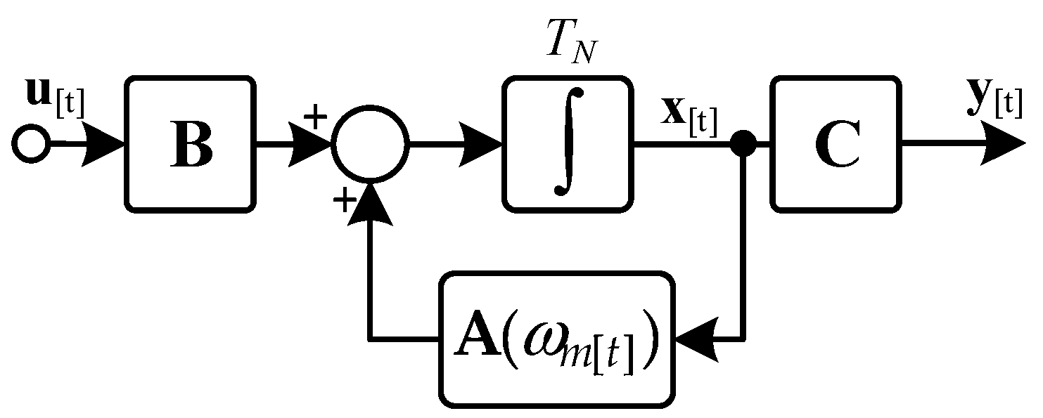
2.1. Mathematical Model of the Induction Motor

The mathematical model of the IM is usually formulated using the following simplifying assumptions [3]:

• The stator and rotor cage windings are considered concentrated windings;
• The machine is treated as an ideal three-phase symmetrical motor;
• The air gap is assumed to be uniform;
• The effects of anisotropy, magnetic saturation, hysteresis phenomena, and eddy currents are neglected;
• Higher harmonics of the spatial field distribution in the air gap are neglected (only the fundamental harmonic is considered);
• Resistances and inductances of the machine windings are treated as constant.

After adopting these commonly used assumptions and spatial vectors for electromagnetic state variables, the mathematical model of the IM can be presented in the stationary coordinate system (α–β), in relative units [p.u.] in the form of the state equation:

$$T_N\frac{\mathrm{d}}{\mathrm{d}t}{x}_{[t]}=A\left({\omega }_{m[t]}\right)x_{[t]}+B{u}_{[t]},$$

(1)

$$y_{[t]}=C{x}_{[t]},$$

(2)

where x—state vector, y—measurement (output) vector, u—control (input) vector, A(ω_m[t])—state matrix, which depends on the motor speed ω_m, B—control (input) matrix, C—output matrix, and T_N—normalizing time constant: T_N = 1/(2πf_sN) [s]. The lower subscript in square brackets defines the calculation time.

A schematic diagram of the mathematical model of the IM expressed by Equations (1) and (2) is shown in Figure 1.

Taking the state vector as

$$x_{[t]}={\left[\begin{array}{cccc}{i}_{s\alpha [t]}& i_{s\beta [t]}& {\Psi }_{r\alpha [t]}& {\Psi }_{r\beta [t]}\end{array}\right]}^T,$$

(3)

Equation (1) and (2) are expressed as follows:

$$T_N\frac{\mathrm{d}}{\mathrm{d}t}\underset{x_{[t]}}{\underbrace{\left[\begin{array}{c}{i}_{s\alpha [t]}\\ i_{s\beta [t]}\\ {\Psi }_{r\alpha [t]}\\ {\Psi }_{r\beta [t]}\end{array}\right]}}=\underset{A\left({\omega }_{m[t]}\right)}{\underbrace{\left[\begin{array}{cccc}{a}_1{r}_s+a_2{r}_r& 0& a_3{r}_r& a_4{\omega }_{m[t]}\\ 0& a_1{r}_s+a_2{r}_r& -a_4{\omega }_{m[t]}& a_3{r}_r\\ a_5{r}_r& 0& a_6{r}_r& -{\omega }_{m[t]}\\ 0& a_5{r}_r& {\omega }_{m[t]}& a_6{r}_r\end{array}\right]}}\underset{x_{[t]}}{\underbrace{\left[\begin{array}{c}{i}_{s\alpha [t]}\\ i_{s\beta [t]}\\ {\Psi }_{r\alpha [t]}\\ {\Psi }_{r\beta [t]}\end{array}\right]}}+\underset{B}{\underbrace{\frac{1}{\sigma l_s}{\left[\begin{array}{cccc}1& 0& 0& 0\\ 0& 1& 0& 0\end{array}\right]}^T}}\underset{u_{[t]}}{\underbrace{\left[\begin{array}{c}{u}_{s\alpha [t]}\\ u_{s\beta [t]}\end{array}\right]}},$$

(4)

$$\underset{y_{[t]}}{\underbrace{\left[\begin{array}{c}{i}_{s\alpha [t]}\\ i_{s\beta [t]}\end{array}\right]}}=\underset{C}{\underbrace{\left[\begin{array}{cccc}1& 0& 0& 0\\ 0& 1& 0& 0\end{array}\right]}}\underset{x_{[t]}}{\underbrace{\left[\begin{array}{c}{i}_{s\alpha [t]}\\ i_{s\beta [t]}\\ {\Psi }_{r\alpha [t]}\\ {\Psi }_{r\beta [t]}\end{array}\right]}},$$

(5)

where $a_1=-\frac{1}{\sigma l_s},a_2=-\frac{1-\sigma }{\sigma l_r},a_3=\frac{l_m}{\sigma l_s{l}_r^2},a_4=\frac{l_m}{\sigma l_s{l}_r},a_5=\frac{l_m}{l_r},a_6=-\frac{1}{l_r}$ and r_s and r_r—stator and rotor resistance, l_m, l_s, and l_r—main, stator, and rotor inductances, respectively, and σ = 1 − l_m²/(l_sl_r)—total leakage factor.

2.2. Mathematical Model of the Extended Kalman Filter

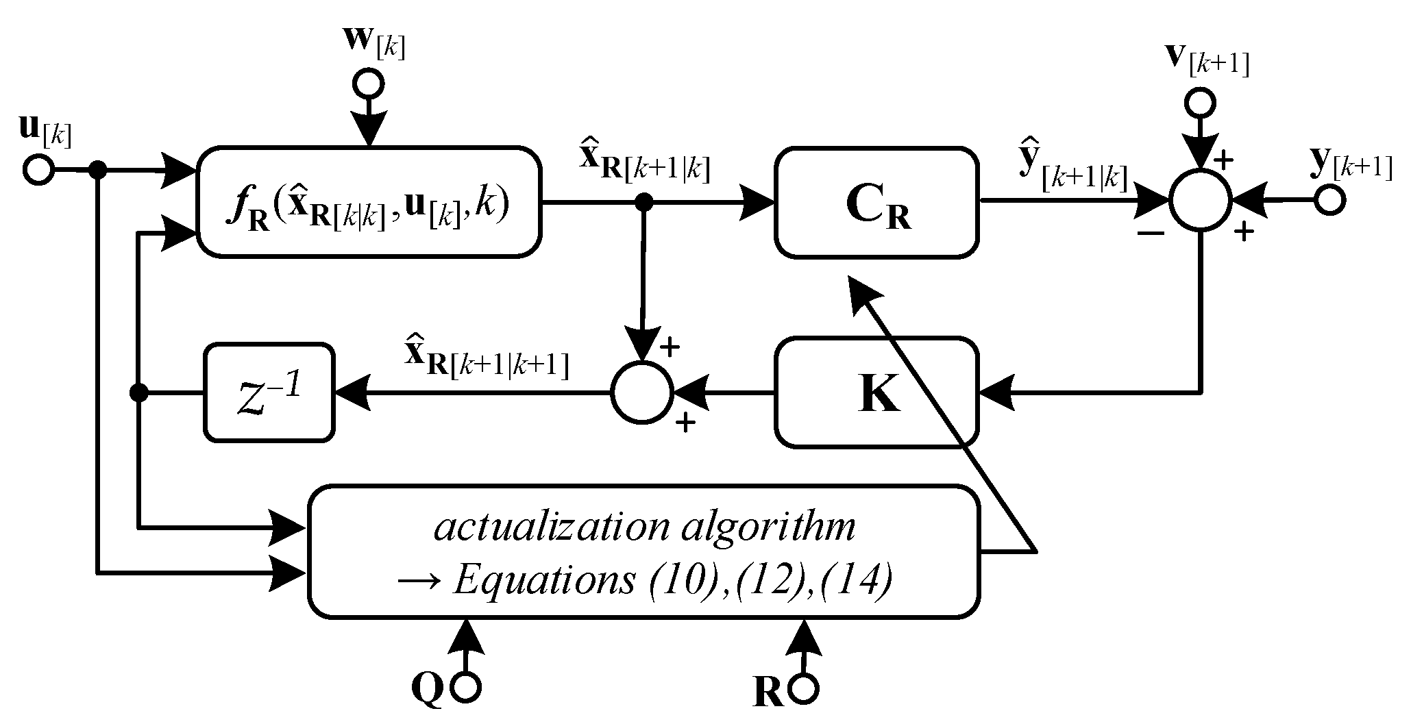
2.2.1. General Model and the Calculation Algorithm of the Extended Kalman Filter

According to the KF theory, the IM model should be written in a discrete form, and noise signals should be included [27]. Moreover, when the state vector (3) is extended with an additional element (rotor speed, stator resistance, rotor resistance, etc.), Equation (4) becomes nonlinear. Consequently, the mathematical model of the IM is expressed as follows:

$$x_{R[k+1]}=f_R\left[x_{R[k]},u_{[k]},k\right]+G_{[k]}{w}_{[k]}=A_R\left(x_{R[k]},k\right)x_{R[k]}+B_{R[k]}{u}_{[k]}+G_{[k]}{w}_{[k]},$$

(6)

$$y_{R[k+1]}=C_{R[k+1]}{x}_{R[k+1]}+v_{[k+1]},$$

(7)

where x_R—extended state vector, G—interference gain coefficient matrix, f_R—a function that constitutes the nonlinear part of the model, and w and v—disturbance matrix of state variables and measurements, respectively.

Regarding noises w and v, it is assumed that they are white, Gaussian, independent noises, with expected values equal to zero, with covariances Q and R, respectively. Therefore

$$\begin{array}{cc}w\sim N\left(0,Q\right),& v\sim N\left(0,R\right).\end{array}$$

(8)

Considering the above assumptions, the EKF algorithm used for the calculation of the extended state vector elements can be presented in the following steps:

• Step 1—calculation of the value of the state vector predictor at the sampling step (k + 1) based on the input u_[k] and the state estimate ${\widehat{x}}_{R[k|k]}$ at the previous moment (k):

  $${\widehat{x}}_{R[k+1|k]}=f_R\left[{\widehat{x}}_{R[k|k]},u_{[k]},k\right]=A_R\left({\widehat{x}}_{R[k|k]},k\right){\widehat{x}}_{R[k|k]}+B_{R[k]}{u}_{[k]},$$

  (9)
• Step 2—calculation of the state prediction error covariance matrix:

  $$P_{[k+1|k]}=F_{[k]}{P}_{[k|k]}{F}_{[k]}^T+Q_{[k]},$$

  (10)

where

$$F_{[k]}={\left.\frac{\partial f_R\left[x_{R[k|k]},u_{[k]},k\right]}{\partial x_{R[k|k]}}\right|}_{x_{R[k|k]}={\widehat{x}}_{R[k|k]}},$$

(11)

And F_[k]—state matrix of the linearized system for the estimate value calculated in the previous step.

• Step 3—calculation of the EKF gain matrix:

  $$K_{[k+1]}=P_{[k+1|k]}{C}_{R[k+1]}^T{\left[C_{R[k+1]}{P}_{[k+1|k]}{C}_{R[k+1]}^T+R\right]}^{-1},$$

  (12)
• Step 4—calculation of the adjusted state vector estimate:

  $${\widehat{x}}_{R[k+1|k+1]}={\widehat{x}}_{R[k+1|k]}+K_{[k+1]}\left[y_{[k+1]}-C_{R[k+1]}{\widehat{x}}_{R[k+1|k]}\right],$$

  (13)

where y_[k+1]—measurements at the present moment (k + 1),

• Step 5—calculation of the estimate error covariance matrix:

  $$P_{[k+1|k+1]}=\left[I-K_{[k+1]}{C}_{R[k+1]}\right]P_{[k+1|k]},$$

  (14)

where I—identity matrix.

• Step 6—back to step one.

To implement the algorithm, it is necessary to select the initial matrices: x_[0|0] and P_[0|0]. However, the appropriate choice of Q and R matrices is crucial. They determine the quality and rate of the estimation process [20,28,29].

The schematic diagram of the extended Kalman filter is shown in Figure 2.

2.2.2. Mathematical Model of the Classical Extended Kalman Filters for Rotor Resistance Estimation

When the state vector contains the electromagnetic state variables and rotor resistance:

$${\widehat{x}}_{R[k]}^r={\left[\begin{array}{ccccc}{\widehat{i}}_{s\alpha [k]}& {\widehat{i}}_{s\beta [k]}& {\widehat{\Psi }}_{r\alpha [k]}& {\widehat{\Psi }}_{r\beta [k]}& {\widehat{r}}_{r[k]}\end{array}\right]}^T,$$

(15)

The discretized (with step T_p) mathematical model of the IM can be described by Equations (6) and (7), whereby

• Output vector:

  $${\widehat{y}}_{R[k]}={\left[\begin{array}{cc}{\widehat{i}}_{s\alpha [k]}& {\widehat{i}}_{s\beta [k]}\end{array}\right]}^T,$$

  (16)
• Input vector:

  $$u_{R[k]}={\left[\begin{array}{cc}{u}_{s\alpha [k]}& u_{s\beta [k]}\end{array}\right]}^T,$$

  (17)

And

• Extended output matrix:

  $$C_R=\left[\begin{array}{ccccc}1& 0& 0& 0& 0\\ 0& 1& 0& 0& 0\end{array}\right],$$

  (18)
• Extended input matrix:

  $$B_R=\frac{T_p}{\sigma l_s{T}_N}{\left[\begin{array}{ccccc}1& 0& 0& 0& 0\\ 0& 1& 0& 0& 0\end{array}\right]}^T,$$

  (19)
• Extended state matrix:

  $$A_{R[k]}^r=I+\frac{T_p}{T_N}\left[\begin{array}{ccccc}{a}_1{r}_s+a_2{\widehat{r}}_{r[k]}& 0& a_3{r}_{r[k]}& a_4{\omega }_{m[k]}& 0\\ 0& a_1{r}_s+a_2{\widehat{r}}_{r[k]}& -a_4{\omega }_{m[k]}& a_3{r}_{r[k]}& 0\\ a_5{\widehat{r}}_{r[k]}& 0& a_6{r}_{r[k]}& -{\omega }_{m[k]}& 0\\ 0& a_5{\widehat{r}}_{r[k]}& {\omega }_{m[k]}& a_6{r}_{r[k]}& 0\\ 0& 0& 0& 0& 0\end{array}\right],$$

  (20)

The state matrix of the linearized system for the estimated value calculated in the previous step takes the following form:

$$F_{[k]}^r=I+\frac{T_p}{T_N}\left[\begin{array}{ccccc}{a}_1{r}_s+a_2{\widehat{r}}_{r[k]}& 0& a_3{r}_{r[k]}& a_4{\omega }_{m[k]}& a_2{\widehat{i}}_{s\alpha [k]}+a_3{\widehat{\Psi }}_{r\alpha [k]}\\ 0& a_1{r}_s+a_2{\widehat{r}}_{r[k]}& -a_4{\omega }_{m[k]}& a_3{r}_{r[k]}& a_2{\widehat{i}}_{s\beta [k]}+a_3{\widehat{\Psi }}_{r\beta [k]}\\ a_5{\widehat{r}}_{r[k]}& 0& a_6{r}_{r[k]}& -{\omega }_{m[k]}& a_5{\widehat{i}}_{s\alpha [k]}+a_6{\widehat{\Psi }}_{r\alpha [k]}\\ 0& a_5{\widehat{r}}_{r[k]}& {\omega }_{m[k]}& a_6{r}_{r[k]}& a_5{\widehat{i}}_{s\beta [k]}+a_6{\widehat{\Psi }}_{r\beta [k]}\\ 0& 0& 0& 0& 0\end{array}\right].$$

(21)

2.2.3. Mathematical Models of the Modified Extended Kalman Filters for Rotor and Stator Resistance Estimation

In this research, two modified EKFs are tested: EKF₁—for the estimation of α, β components of the stator current and rotor flux vectors and additionally the coefficient representing uncertainties of the rotor resistance (relative to the rated value); and EKF₂—for the estimation of components of the stator current and rotor flux vectors and general factor of changes in both rotor and stator resistances versus their nominal values.

In the case of EKF₁, the last element of the state vector (15) is replaced by the relative rotor resistance change factor, defined as follows, similarly to in [28,29]:

$$d_r=\frac{r_r^{real}}{r_{rN}},$$

(22)

where r_r^real and r_rN —actual and rated rotor resistance, respectively.

Therefore, d_r takes values of the same order of magnitude as the stator currents and rotor fluxes. For such modification, the state vector and matrices A_R and F_R for EKF₁ take the following form of Equations (23)–(25):

$${\widehat{x}}_{R[k]}^{dr}={\left[\begin{array}{ccccc}{\widehat{i}}_{s\alpha [k]}& {\widehat{i}}_{s\beta [k]}& {\widehat{\Psi }}_{r\alpha [k]}& {\widehat{\Psi }}_{r\beta [k]}& {\widehat{d}}_{r[k]}\end{array}\right]}^T,$$

(23)

$$A_{R[k]}^{dr}=I+\frac{T_p}{T_N}\left[\begin{array}{ccccc}{a}_1{r}_s+a_2{r}_r{\widehat{d}}_{r[k]}& 0& a_3{r}_r{d}_{r[k]}& a_4{\omega }_{m[k]}& 0\\ 0& a_1{r}_s+a_2{r}_r{\widehat{d}}_{r[k]}& -a_4{\omega }_{m[k]}& a_3{r}_r{d}_{r[k]}& 0\\ a_5{r}_r{\widehat{d}}_{r[k]}& 0& a_6{r}_r{d}_{r[k]}& -{\omega }_{m[k]}& 0\\ 0& a_5{r}_r{\widehat{d}}_{r[k]}& {\omega }_{m[k]}& a_6{r}_r{d}_{r[k]}& 0\\ 0& 0& 0& 0& 0\end{array}\right],$$

(24)

$$F_{[k]}^{dr}=I+\frac{T_p}{T_N}\left[\begin{array}{ccccc}{a}_1{r}_s+a_2{r}_r{\widehat{d}}_{r[k]}& 0& a_3{r}_r{d}_{r[k]}& a_4{\omega }_{m[k]}& \left(a_2{\widehat{i}}_{s\alpha [k]}+a_3{\widehat{\Psi }}_{r\alpha [k]}\right)r_r\\ 0& a_1{r}_s+a_2{r}_r{\widehat{d}}_{r[k]}& -a_4{\omega }_{m[k]}& a_3{r}_r{d}_{r[k]}& \left(a_2{\widehat{i}}_{s\beta [k]}+a_3{\widehat{\Psi }}_{r\beta [k]}\right)r_r\\ a_5{r}_r{\widehat{d}}_{r[k]}& 0& a_6{r}_r{d}_{r[k]}& -{\omega }_{m[k]}& \left(a_5{\widehat{i}}_{s\alpha [k]}+a_6{\widehat{\Psi }}_{r\alpha [k]}\right)r_r\\ 0& a_5{r}_r{\widehat{d}}_{r[k]}& {\omega }_{m[k]}& a_6{r}_r{d}_{r[k]}& \left(a_5{\widehat{i}}_{s\beta [k]}+a_6{\widehat{\Psi }}_{r\beta [k]}\right)r_r\\ 0& 0& 0& 0& 0\end{array}\right].$$

(25)

During drive operation, both the stator and the rotor resistance change mainly due to temperature variations. Taking into account the fact that the temperature coefficients of changes in the resistance of aluminum (the material of the rotor cage) and copper (for the stator winding) are almost identical, it can be assumed that changes in stator resistance as a function of temperature are proportional to changes in rotor resistance, on this account:

$$d_{r,s}=\frac{r_r^{real}}{r_{rN}}=\frac{r_s^{real}}{r_{sN}}=d.$$

(26)

With this assumption, it is possible to implement a motor model extended by a single resistance change coefficient d_r,s = d, concerning both the stator and rotor resistance, and thus obtain an EKF₂—the filter for estimating electromagnetic state variables and both stator and rotor resistances. This approach allows both resistances to be updated simultaneously while keeping the algorithm simple and low order (fifth—as in EKF₁). For such a modification, the state vector and suitable matrices A_R and F_R for EKF₂ are expressed as follows in Equations (27)–(29):

$${\widehat{x}}_{R[k]}^d={\left[\begin{array}{ccccc}{\widehat{i}}_{s\alpha [k]}& {\widehat{i}}_{s\beta [k]}& {\widehat{\Psi }}_{r\alpha [k]}& {\widehat{\Psi }}_{r\beta [k]}& {\widehat{d}}_{[k]}\end{array}\right]}^T,$$

(27)

$$A_{R[k]}^d=I+\frac{T_p}{T_N}\left[\begin{array}{ccccc}{a}_1{r}_s{\widehat{d}}_{[k]}+a_2{r}_r{d}_{[k]}& 0& a_3{r}_r{\widehat{d}}_{[k]}& a_4{\omega }_{m[k]}& 0\\ 0& a_1{r}_s{\widehat{d}}_{[k]}+a_2{r}_r{d}_{[k]}& -a_4{\omega }_{m[k]}& a_3{r}_r{\widehat{d}}_{[k]}& 0\\ a_5{r}_r{\widehat{d}}_{[k]}& 0& a_6{r}_r{d}_{[k]}& -{\omega }_{m[k]}& 0\\ 0& a_5{r}_r{\widehat{d}}_{[k]}& {\omega }_{m[k]}& a_6{r}_r{d}_{[k]}& 0\\ 0& 0& 0& 0& 0\end{array}\right],$$

(28)

$$F_{[k]}^d=I+\frac{T_p}{T_N}\left[\begin{array}{ccccc}{a}_1{r}_s{\widehat{d}}_{[k]}+a_2{r}_r{d}_{[k]}& 0& a_3{r}_r{\widehat{d}}_{[k]}& a_4{\omega }_{m[k]}& \left(a_1{r}_s+a_2{r}_r\right){\widehat{i}}_{s\alpha [k]}+a_3{r}_r{\widehat{\Psi }}_{r\alpha [k]}\\ 0& a_1{r}_s{\widehat{d}}_{[k]}+a_2{r}_r{d}_{[k]}& -a_4{\omega }_{m[k]}& a_3{r}_r{\widehat{d}}_{[k]}& \left(a_1{r}_s+a_2{r}_r\right){\widehat{i}}_{s\beta [k]}+a_3{r}_r{\widehat{\Psi }}_{r\beta [k]}\\ a_5{r}_r{\widehat{d}}_{[k]}& 0& a_6{r}_r{d}_{[k]}& -{\omega }_{m[k]}& \left(a_5{\widehat{i}}_{s\alpha [k]}+a_6{\widehat{\Psi }}_{r\alpha [k]}\right)r_r\\ 0& a_5{r}_r{\widehat{d}}_{[k]}& {\omega }_{m[k]}& a_6{r}_r{\widehat{d}}_{[k]}& \left(a_5{\widehat{i}}_{s\beta [k]}+a_6{\widehat{\Psi }}_{r\beta [k]}\right)r_r\\ 0& 0& 0& 0& 0\end{array}\right].$$

(29)

It should be emphasized that the parameters r_s and r_r in the respective matrices given by Equations (24), (25), (28), and (29) are treated as constant, and are rated just like the other parameters in the coefficients a₁–a₆. The input and output vectors and matrices for EKF₁ and EKF₂ take the form of Equations (16)–(19).

3. Research Scenarios

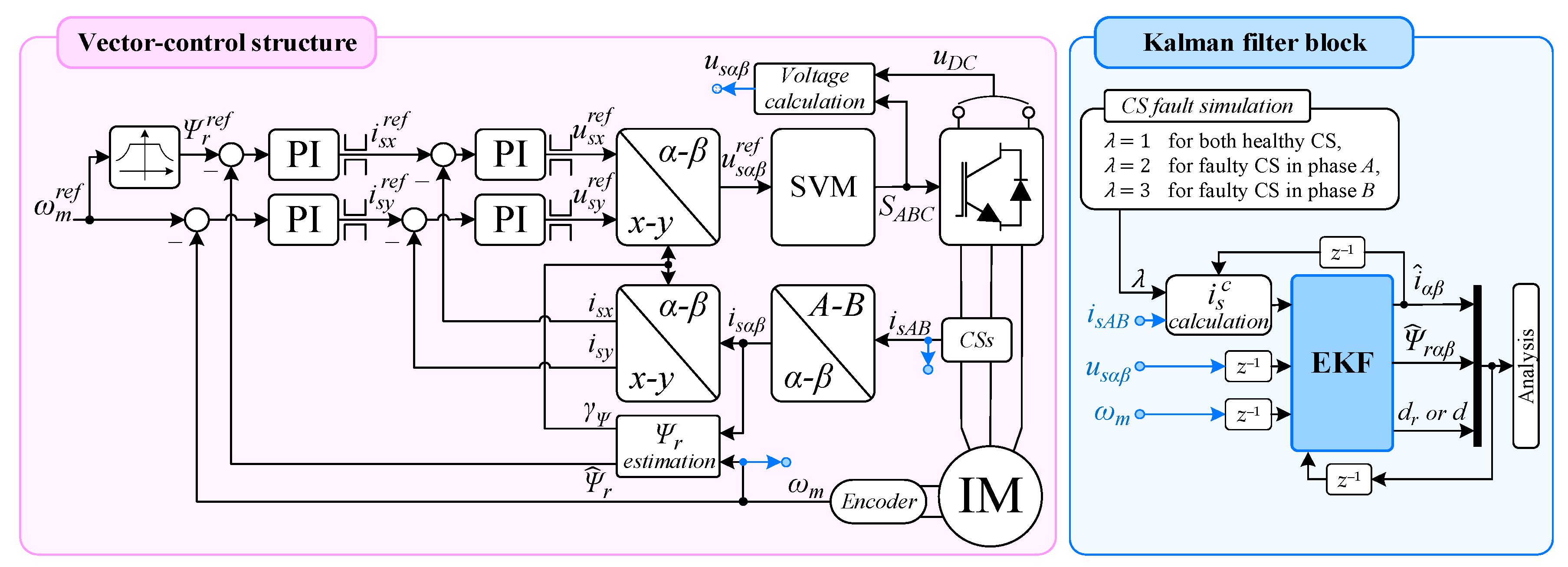
3.1. Simulation Details and Research Scenarios

All tests were carried out for a drive system with an IM controlled by the Direct Field-Oriented Control (DFOC) method, with two CSs applied in the control structure. The rated parameters of the IM are presented in Appendix A. To reliably assess the quality of stator current estimation by the proposed EKF₁ and EKF₂, it is assumed that the variables estimated by the EKF do not interfere with the drive control system (the estimator works in an open loop). Moreover, CS faults are only simulated at the EKF input. Thus, measured, undisturbed by faulty CS currents are used to implement the current feedback required in the DFOC structure.

In the situation where any of the CS fails, the current signal is no longer available (or is clearly distorted). Therefore, to provide the best quality of EKF estimation, at the EKF input, the measured currents i_sAB are converted to the stationary reference frame (α–β) and then replaced by the corrected current components $i_{s\alpha \beta }^c$. They are a combination of phase currents measured by healthy CSs and the currents ${\widehat{i}}_{sABC}$, estimated by a given EKF. Thus, corrected currents are calculated depending on the location of the damage (indicated by the λ factor) as follows:

$$\left[\begin{array}{c}{\widehat{i}}_{s\alpha }^c\\ {\widehat{i}}_{s\beta }^c\end{array}\right]=\left\{\begin{array}{ccc}\left[\begin{array}{c}{i}_{sA}\\ \frac{\sqrt{3}}{3}\left(i_{sA}+2i_{sB}\right)\end{array}\right]& \mathrm{for}& \mathrm{both} \mathrm{healthy} \mathrm{CS} \left(\lambda =1\right)\\ \left[\begin{array}{c}-i_{sB}-{\widehat{i}}_{sC}\\ \frac{\sqrt{3}}{3}\left({\widehat{i}}_{sA}+2i_{sB}\right)\end{array}\right]& \mathrm{for}& \mathrm{faulty} \mathrm{CS} \mathrm{in} \mathrm{phase} A\left(\lambda =2\right)\\ \left[\begin{array}{c}{i}_{sA}\\ \frac{\sqrt{3}}{3}\left(i_{sA}+2{\widehat{i}}_{sB}\right)\end{array}\right]& \mathrm{for}& \mathrm{faulty} \mathrm{CS} \mathrm{in} \mathrm{phase} B\left(\lambda =3\right)\end{array},\right.$$

(30)

Estimated phase currents are calculated based on estimated currents, ${\widehat{i}}_{s\alpha \beta }$, using the inverse Clarke transform:

$$\left[\begin{array}{c}{\widehat{i}}_{sA}\\ {\widehat{i}}_{sB}\\ {\widehat{i}}_{sC}\end{array}\right]=\left[\begin{array}{cc}1& 0\\ -\frac{1}{2}& \frac{\sqrt{3}}{2}\\ -\frac{1}{2}& -\frac{\sqrt{3}}{2}\end{array}\right]\left[\begin{array}{c}{\widehat{i}}_{s\alpha }\\ {\widehat{i}}_{s\beta }\end{array}\right].$$

(31)

The components of the stator voltage u_s, required by the EKF algorithm, are calculated based on the actual switching states S_ABC of the inverter IGBTs and on the measurement of the DC-bus voltage, u_DC, according to the equation:

$$\left[\begin{array}{c}{u}_{s\alpha }\\ u_{s\beta }\end{array}\right]=\frac{1}{3}{u}_{DC}\left[\begin{array}{c}2S_A-S_B-S_C\\ \sqrt{3}\left(S_B-S_C\right)\end{array}\right].$$

(32)

The general functional diagram of the tested system is shown in Figure 3.

The system simulation models were performed using the MATLAB/Simulink 2023b software. The Euler method (ode1) was used to numerically solve differential equations, with a sampling time of 6.25 μs. The modulation frequency was assumed to be 8 kHz. To reproduce the simulation conditions as close as possible to the real ones, the presence of measurement noise of the stator current, DC-bus voltage u_DC of the voltage source inverter (VSI), and the IM angular speed were assumed. The current noise was modeled based on an actual measurement performed under rated operating conditions.

The noise parameters were selected by analyzing the frequency spectrum obtained using a fast Fourier transform. (FFT) of the stator current signal. It was assumed that the measurement noise was white, Gaussian with a zero expected value. The variance was selected to receive a spectrum close to the real one, thus maintaining the noise signal at −70 dB (variance assumed: 7.5 × 10⁻⁵). A graphical FFT representation of both signals, real (measured) and simulated, is shown in Figure 4. Since voltage measurement is carried out using a measuring transducer of the same type, the presence of the same noise was assumed. The measurement noise on the encoder was considered a pulse counting error, which was implemented in accordance with [9]. Example waveforms of noisy and ideal signals are shown in Figure 5.

3.2. Methodology for Testing the Quality of Stator Current Estimation Using EKFs

The research on the proposed EKFs was divided into two stages:

−

first, the influence of the elements of the Q matrix for EKF₁ on the quality of state variable estimation, in particular the stator current, in the presence of changes in the IM parameters and the occurrence of CS damages in phases A and B of the stator winding;

−

then, considering the conclusions resulting from the first stage of research, the quality of stator current estimation provided by EKF₁ and EKF₂ was compared.

The following assumptions were made for these tests:

• The matrix R is considered constant and diagonal, with a value determined according to [30] as: $R=diag\left[\begin{array}{cc}7.5\times {10}^{-5}& 1.25\times {10}^{-4}\end{array}\right]$;
• Initial conditions for EKFs: $P_{[0|0]}=diag\left[\begin{array}{cccc}{10}^{-3}& {10}^{-3}& {10}^{-3}& \begin{array}{cc}{10}^{-3}& {10}^{-5}\end{array}\end{array}\right]$, $x_{[0|0]}=diag\left[\begin{array}{cccc}0& 0& 0& \begin{array}{cc}0& 1\end{array}\end{array}\right]$;
• Matrix Q is diagonal;
• the influence of only elements q₁₁ and q₂₂ of the Q matrix is examined, each of which can have values in the following range: $q=\left\{\begin{array}{cccc}{10}^{-7},& {10}^{-8},& 8\times {10}^{-9},& \begin{array}{cc}{10}^{-9},& {10}^{-10}\end{array}\end{array}\right\}$; these values mostly influence the current estimation quality;
• The remaining elements of the Q matrix (q₃₃, q₄₄, and q₅₅) are considered constants, with values 10⁻¹⁰;
• The tests are carried out for both motoring and regenerating mode, for speed range ${\omega }_m^{ref}=\{\pm 0.01,\pm 1\}{\omega }_{mN}$, and load torque $t_L=\{0.05,1\}{t}_{LN}$, assuming changes in the motor model parameters (r_r, r_s, and l_m) within the range of ± 25% of the rated value for three fault situations: failure-free (λ = 1), with CS damage in phase A (λ = 2) and with damage in phase B (λ = 3);
• Additionally, the situation in which both the stator and the rotor resistance changes is considered. The parameters were changed only in the motor model.

4. Analysis of the Results

4.1. Influence of the Q Matrix for EKF₁ on the Quality of Current Estimation

According to the defined assumption, in this stage of the research, the best pair of q₁₁ and q₂₂ at a given operating point of the drive system was determined based on the selection criterion, defined as the average of the root mean square error (RMSE) value for the phase currents (i_sA, i_sB):

$$\delta i_{sAB}=\frac{1}{2}\left(\sqrt{\frac{{\displaystyle \sum _{k=t_1/T_p}^{t_2/T_p}{\left(i_{sA}(k)-{\widehat{i}}_{sA}(k)\right)}^2}}{\frac{\left(t_2-t_1\right)}{T_p}+1}}+\sqrt{\frac{{\displaystyle \sum _{k=t_1/T_p}^{t_2/T_p}{\left(i_{sB}(k)-{\widehat{i}}_{sB}(k)\right)}^2}}{\frac{\left(t_2-t_1\right)}{T_p}+1}}\right).$$

(33)

where ${\widehat{i}}_{sA[k]}$ and ${\widehat{i}}_{sB[k]}$—estimated phase currents,$i_{sA[k]}$ and $i_{sB[k]}$—measured ideal currents (without noise added), and t₁ and t₂—the beginning and end of the analyzed time interval (for this study: 10 s of the steady state).

It should be noted that considering ideal measured currents (without measurement uncertainties) in Equation (33) makes it possible to find a Q matrix that provides the best properties for filtering measurement noise. Moreover, EKF uses corrected currents Equation (30) which are created from the available (after fault) measured current (with noise added) and estimated ones. Because RMSEs are calculated for changes in three parameters of the motor model, it is possible to determine the Q that provides the best robustness to all of their changes. Thus, the final error at a given operating point is calculated as the average of RMSE for all parameter changes.

In

Table 2. Average RMSE values for current, δi_sAB, for all parameter changes, and with CS damage in phase A under motoring mode (multiplied by 10³).

q11/q22	1% of ωmN					100% of ωmN					Load Torque tL
	10−7	10−8	8 × 10−9	10−9	10−10	10−7	10−8	8 × 10−9	10−9	10−10
10−7	16.25	18.41	18.77	21.36	22.48	10.16	9.17	9.17	9.19	9.20	tL = 5%
10−8	16.61	14.64	14.72	16.61	17.90	9.10	4.94	4.84	4.67	4.69
8 × 10−9	16.73	14.51	14.54	16.22	17.47	9.12	4.74	4.62	4.44	4.46
10−9	17.40	14.35	14.14	14.24	15.39	9.33	3.91	3.73	3.55	3.70
10−10	17.33	14.07	13.79	13.36	X	9.39	3.79	3.59	3.60	4.07
10−7	20.19	25.67	26.60	35.07	39.98	27.07	21.33	21.18	20.60	20.51	tL = 100%
10−8	24.33	20.42	20.62	26.76	32.93	19.79	11.49	11.18	10.19	10.09
8 × 10−9	24.92	20.45	20.56	26.06	32.18	19.42	10.95	10.62	9.57	9.48
10−9	28.05	23.19	22.80	23.39	28.48	17.68	8.46	7.96	6.18	6.12
10−10	28.45	25.33	24.99	24.39	32.32	17.34	8.04	7.51	5.71	6.03

Blue color—lowest value; red color—values exceeding 20 × 10⁻³; grey color—100 × 10⁻³.

and

Table 3. Average RMSE values for current, δi_sAB, for all parameter changes, and with CS damage in phase A under regenerating mode (multiplied by 10³).

q11/q22	1% of ωmN					100% of ωmN					Load Torque tL
	10−7	10−8	8 × 10−9	10−9	10−10	10−7	10−8	8 × 10−9	10−9	10−10
10−7	17.57	21.51	21.94	25.43	26.29	11.63	9.02	8.93	8.63	8.60	tL = 5%
10−8	16.96	17.83	17.91	X	X	12.11	6.69	6.38	4.92	4.66
8 × 10−9	17.01	18.25	18.36	X	X	12.20	6.68	6.35	4.79	4.51
10−9	17.51	19.57	21.36	X	X	12.72	6.96	6.59	4.47	4.01
10−10	17.77	18.87	19.86	38.53	X	12.85	7.09	6.72	4.53	3.99
10−7	20.16	26.24	27.28	36.75	42.79	30.55	23.71	23.53	22.90	22.82	tL = 100%
10−8	25.18	20.93	21.15	27.59	33.85	22.05	12.51	11.93	9.14	8.63
8 × 10−9	25.91	21.06	21.18	27.00	33.11	21.65	12.21	11.62	8.60	8.03
10−9	29.66	24.50	24.15	26.74	32.76	19.59	11.43	10.83	6.88	5.83
10−10	29.49	26.19	25.92	97.56	X	19.15	11.38	10.82	6.85	5.67

Blue color—lowest value; red color—values exceeding 20 × 10⁻³; grey color—100 × 10⁻³.

, examples of the average current RMSE values for different operating points in motoring and regenerating modes are presented. The lowest values for a given operating point are marked in blue, values exceeding 20 × 10⁻³ are marked in red, and unstable points (or when the error exceeds 100 × 10⁻³) are marked in grey.

Similar results were obtained in the case of a CS fault in phase B. For the failure-free case, the RMSE values of the current range from 1.27 × 10⁻³ to 16.89 × 10⁻³.

The analysis of the obtained results shows that in a situation where all current sensors are available, the selection of elements q₁₁ and q₂₂ of the Q matrix is not critical to obtain a satisfactory quality of stator current estimation (for all assumed pairs of q elements the estimation errors are similar). Therefore, in the failure-free state, it is sufficient to select one Q matrix constant throughout the entire drive operating range. The influence of the selection of q₁₁ and q₂₂ on the quality of the stator current estimation is observed in the event of failure of any CS, especially in the low speed range (Table 2 and Table 3)—when q values are set too small, the system tends to lose stability. The appropriate selection of the Q matrix also allows the current estimation error to be reduced even several times.

However, as can be seen from this part of the investigation, it is difficult to determine the one pair of $q_{11}$ and $q_{22}$ elements, the best for all operating points of the drive system and CS fault scenarios. Therefore, for further testing of both analyzed EKFs, the parameters that ensure the smallest average RMSE of the current for all operating points and changes in motor parameters were adopted:

• For failure-free CSs: {q₁₁; q₂₂} = {10⁻⁷; 10⁻⁷};
• For sensor damage in phase A or phase B: {q₁₁; q₂₂} = {8 × 10⁻⁹; 8 × 10⁻⁹}.

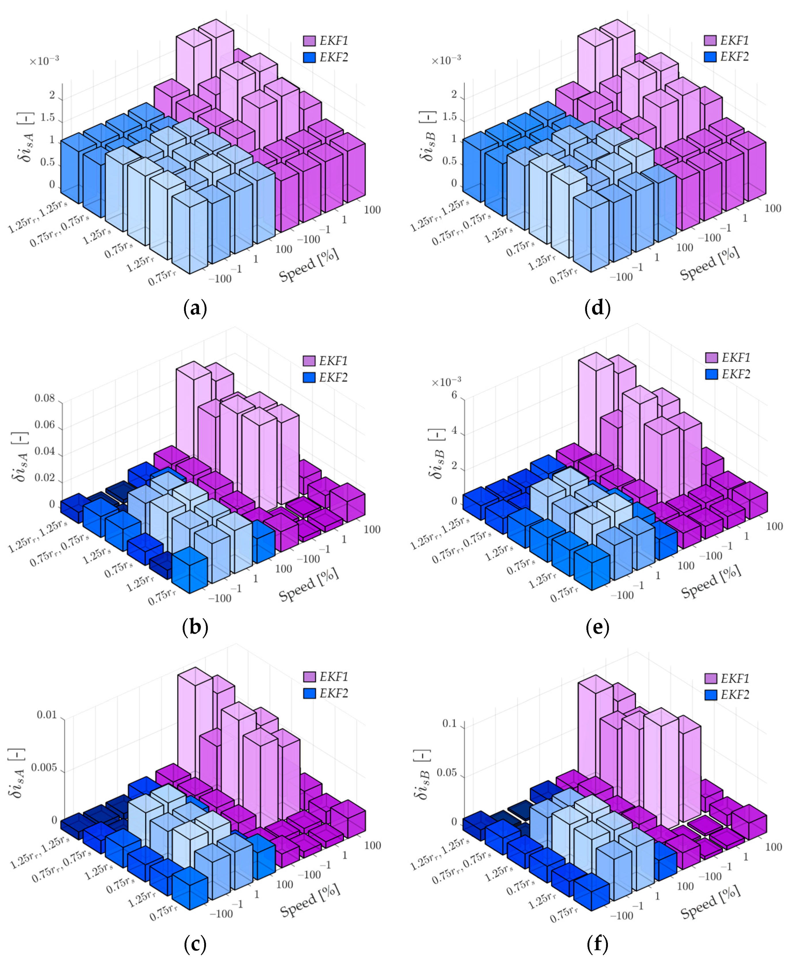
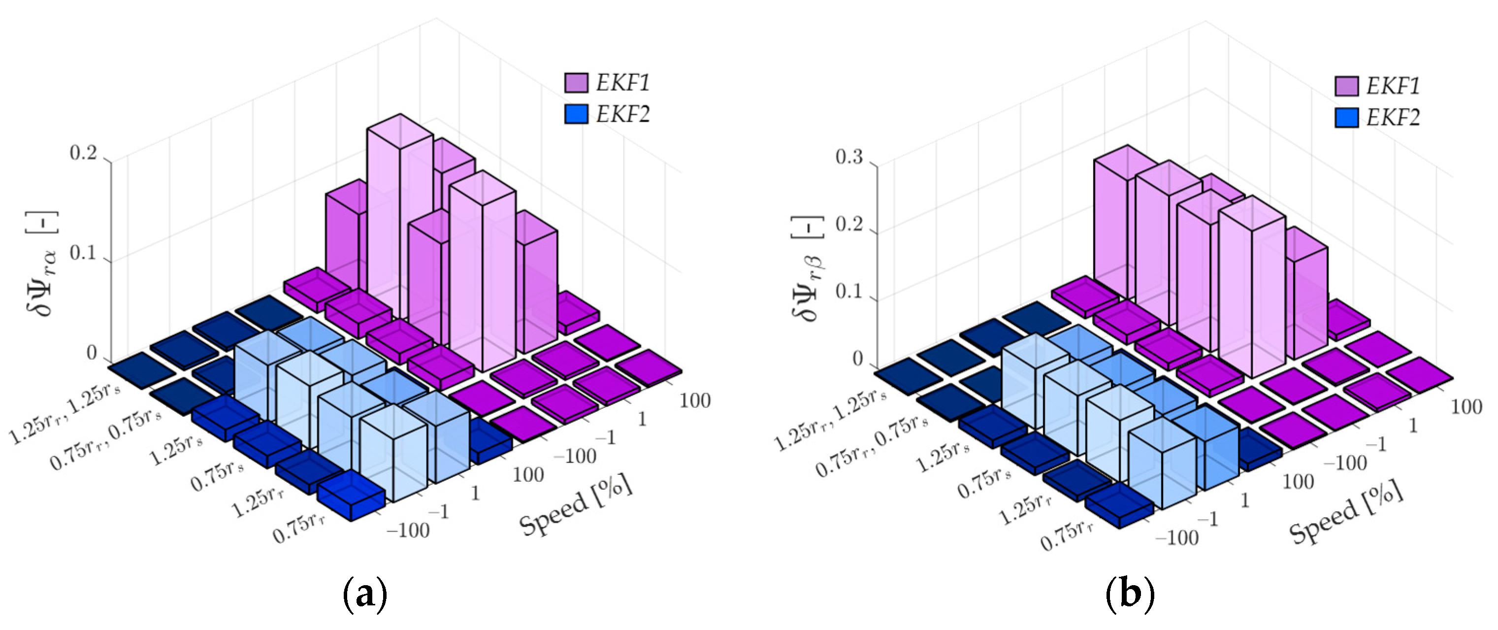
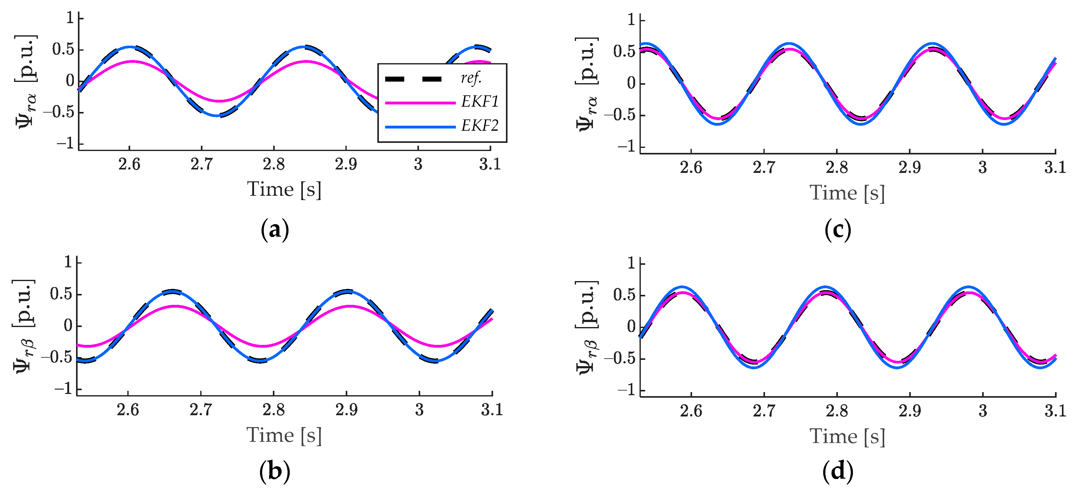
4.2. Analysis of the Quality of Stator Current Estimation Using EKF₁ and EKF₂

In the second stage of the study, the quality of the stator current estimation provided by EKF₁ and EKF₂ was compared. The tests were carried out in various drive operating states (both during motor operation and in regenerating mode) and with different changes in motor resistances. The quality of the estimation of the phase currents was evaluated using RMSE), according to the following equation:

$$\delta i_{sm}=\sqrt{\frac{{\displaystyle \sum _{k=t_1/T_p}^{t_2/T_p}{\left(i_{sm}(k)-{\widehat{i}}_{sm}(k)\right)}^2}}{\frac{\left(t_2-t_1\right)}{T_p}+1}}.$$

(34)

where m—phase A or B.

RMSE values for both tested EKFs, for nominal load, and all CSs statuses are illustrated in Figure 6. Since the IM is operating mostly with a load close to the nominal, it was decided to show the results only for such a load. However, the results obtained for low load torque (5% of its nominal value) take similar (or even smaller) values.

As can be seen, EKF₂, which considers changes in both motor resistances, allows us to decrease current estimation error, especially in low speed regions, when any of the CS is broken. For the rated speed, both models usually provide similar estimation errors.

When all CSs are available, there are no significant differences between both proposed models (Figure 6a,d). Moreover, resistance changes do not considerably affect estimation quality—for all tested operation points and resistance changes, the RMSE of both phase currents are similar and do not exceed 2.5 × 10⁻³. Nonetheless, for some operating points (when stator resistance changes), EKF₂ still provides an estimation error approximately two times smaller than EKF₁.

Analysis of the obtained results shows that the greatest advantage of EKF₂ over EKF₁ becomes apparent when damage to any CS occurs. It can be clearly seen in the low speed region when both the stator and the rotor resistance change simultaneously (Figure 6b,c,e,f).

To quantify the improvement in the estimation when any CS is broken, a percentage improvement in the quality of the current estimation offered by EKF₂ relative to EKF₁ was formulated:

$$\Delta i_{sm}=\frac{\delta i_{sm}^{EK{F}_1}-\delta i_{sm}^{EK{F}_2}}{\delta i_{sm}^{EK{F}_1}}\cdot 100\%.$$

(35)

where m—phase A or B, $\delta i_{sm}^{EK{F}_1}$—RMSE of m-phase current for EKF₁, and $\delta i_{sm}^{EK{F}_2}$—RMSE of m-phase current for EKF₂. The results obtained for CS damage in phases A and B are shown in

Table 4. Improvement in stator phase currents estimation provides for EKF₂ over EKF₁ for CS damage in phase A.

	ΔisA [%]				ΔisB [%]
Resistance/Speed [%]	−100%	−1%	1%	100%	−100%	−1%	1%	100%
rrIM = 0.75 rrN	−36.0	<<−100	<<−100	−16.95	−71.9	<<−100	<<−100	−7.6
rrIM = 1.25 rrN	26.1	<<−100	<<−100	3.66	−75.0	<<−100	<<−100	−57.8
rsIM = 0.75 rsN	11.3	52.5	46.0	4.61	−3.6	50.7	45.2	3.2
rsIM = 1.25 rsN	−4.2	57.0	50.2	−0.28	−4.3	56.4	48.9	1.5
rrIM = 0.75rrN; rsIM = 0.75 rsN	2.8	93.1	91.2	−4.15	28.1	77.0	76.6	33.9
rrIM = 1.25 rrN; rsIM = 1.25 rsN	42.2	97.1	95.6	20.40	21.6	87.6	85.8	13.1

Green color indicates improvement over 20%, and red color points to more than 20% deterioration.

and

Table 5. Improvement in stator phase currents estimation provides for EKF₂ over EKF₁ for CS damage in phase B.

	ΔisA [%]				ΔisB [%]
Resistance/Speed [%]	−100%	−1%	1%	100%	−100%	−1%	1%	100%
rrIM = 0.75 rrN	−73.9	<<−100	<<−100	−32.4	−13.1	<<−100	<<−100	−19.3
rrIM = 1.25 rrN	<<−100	<<−100	<<−100	−29.5	−23.2	<<−100	<<−100	−19.7
rsIM = 0.75 rsN	2.8	53.2	45.6	3.4	6.4	54.9	44.7	2.0
rsIM = 1.25 rsN	−5.5	54.4	46.0	−4.7	−4.2	54.4	46.8	−6.0
rrIM = 0.75 rrN; rsIM = 0.75 rsN	25.2	88.6	88.0	12.3	15.6	95.1	93.8	−2.8
rrIM = 1.25 rrN; rsIM = 1.25 rsN	55.1	94.2	93.0	32.0	12.2	98.3	97.7	5.2

Green color indicates improvement over 20%, and red color points to more than 20% deterioration.

, respectively. Significant improvement (over 20%) is highlighted in green, while the greatest deterioration (less than −20%) is in red.

As can be seen in Table 4 and Table 5, at low angular speeds and when both resistances change, the improvement in the estimation of the current in the phase where the fault occurred is close to 100% (range: 93.1–98.3%), while the other current is estimated from 77.0% to 94.2% better, relative to EKF₁. In addition, the quality of the estimation of missing and available current are similar. As this case is closest to the real situation, it can be concluded that the proposed filter structure EKF₂ will perform better under experimental conditions than the EKF₁ model while maintaining the simplicity of the algorithm.

Each motor parameter is subject to a certain identification error, which means that the actual motor resistance may be far different from that stated on the nameplate. Obviously, such changes may also consider resistances and, in general, affect estimation quality. Therefore, the test was also carried out with changes in only one of the resistances: stator or rotor.

It should be noted that the proposed algorithm EKF₂ makes the estimation process insensitive to any changes in stator resistance. At low speeds, the improvement is up to 57%. Nonetheless, in all operating states in which only the rotor resistance changes, significant deterioration is observed (for low speeds greater than 100%). Therefore, to preserve the best estimation quality using EKF₂, it is necessary to identify the nominal rotor resistance as precisely as possible. However, it is also worth noting that, despite a significant deterioration in estimation quality compared to the EKF₁ model, the error values remain small and satisfactory.

Examples of phase current transients for both filter models (EKF₁ and EKF₂), together with reference signals, for the operating states in which the greatest improvement/deterioration in the quality of current estimation was observed are shown in Figure 7. The greatest improvement in the quality of the estimation of a given phase current (A/B) is observed in the following situation: nominal load, low speed under regenerating mode, when both rotor and stator resistance increase, with faulty CS in the analyzed phase (A/B) (Figure 7a,b). In contrast, the greatest deterioration of quality occurs when only the rotor resistance increases, whereas other conditions remain the same (Figure 7c,d).

It should also be noted that the quality of the DFOC-controlled drive will be influenced not only by the quality of the current estimation but also by the rotor flux components. Therefore, RMSE values calculated for the rotor flux components (in the same way as for the currents) were examined. Results developed for the rated load and for the faulty CS in phase A are shown in Figure 8. The results for the faulty-free case and with fault in phase B are similar.

As it was for currents, it can be clearly seen that EKF₂ allows for the reduction in estimation errors for all situations where stator resistance changes. The greatest improvement and deterioration in the quality of the estimation is observed for the same load and speed as for the current, but in this case, this applies to the fault-free state. The bottom line is that the greatest improvement corresponds to a simultaneous change in both resistances. Consequently, EKF₂ will behave better in a real CS-FTC system, with regard not only to the quality of the current estimation but the entire state vector. The waveforms of the rotor flux components for both EKFs, compared to the reference signal, for the best and worst improvement in the estimation quality of the rotor flux components, are presented in Figure 9.

5. Conclusions

Based on the presented research, the following conclusions can be drawn:

• Correct selection of the Q matrix for the Kalman filter is particularly important in the event of damage to the CS.
• To ensure the highest quality stator current estimation, tuning the Q matrix depending on the current operating point (both speed and load) is recommended.
• The worst quality of estimation is obtained in states characterized by low current variability, which corresponds to operation at low speeds and low loads (especially in regenerating mode).
• Extending the state vector with a general coefficient of resistance change, considering changes in both rotor and stator resistance, allows for increasing the accuracy of the estimation of electromagnetic state variables while maintaining the simplicity of the EKF algorithm. With this approach, a significant deterioration of the estimate occurs only in the case of changes in only the rotor resistance. Since this situation does not occur on a real drive, this defect does not matter.
• The adopted way of calculation of the corrected stator currents, taking into account the available measured and estimated currents makes it possible to properly calculate the state estimation error in the EKF algorithm.

It should be highlighted that the main goal of this work was to develop a Kalman filter for estimating IM stator winding currents in the case of CS fault that would be less sensitive to the most common parametric inaccuracies of the motor model (resistance change during system operation), while maintaining the simplicity of the algorithm, including the relatively low order of the system of equations describing the estimator. The EKF₂ we proposed met these requirements, which was proven by extensive simulation tests. It seems that it may be a good solution as a system for compensating failures to stator current sensors in the drive systems with an increased degree of safety.

To validate the obtained theoretical results, experimental tests will be carried out in the near future.

References

1. Isermann, R. Fault-Diagnosis Applications, Model-Based Condition Monitoring: Actuators, Drives, Machinery, Plants, Sensors, and Fault-Tolerant Systems; Springer: Berlin/Heidelberg, Germany, 2011. [Google Scholar]
2. Muenchhof, M.; Beck, M.; Isermann, R. Fault-tolerant actuators and drives—Structures, fault detection principles and applications. Annu. Rev. Control 2009, 33, 136–148. [Google Scholar] [CrossRef]
3. Orlowska-Kowalska, T.; Kowalski, C.T.; Dybkowski, M. Fault-Diagnosis and Fault-Tolerant-Control in Industrial Processes and Electrical Drives. In Advanced Control of Electrical Drives and Power Electronic Converters; Kabzinski, J., Ed.; Springer: Berlin/Heidelberg, Germany, 2017; pp. 101–120. [Google Scholar] [CrossRef]
4. Dybkowski, M.; Klimkowski, K.; Orlowska-Kowalska, T. Speed and Current Sensor Fault-Tolerant-Control of the Induction Motor Drive. In Advanced Control of Electrical Drives and Power Electronic Converters; Kabzinski, J., Ed.; Springer: Berlin/Heidelberg, Germany, 2017; pp. 141–167. [Google Scholar] [CrossRef]
5. Salmasi, F.R. A Self-Healing Induction Motor Drive with Model Free Sensor Tampering and Sensor Fault Detection, Isolation, and Compensation. IEEE Trans. Ind. Electron. 2017, 64, 6105–6115. [Google Scholar] [CrossRef]
6. Chakraborty, C.; Verma, V. Speed and Current Sensor Fault Detection and Isolation Technique for Induction Motor Drive Using Axes Transformation. IEEE Trans. Ind. Electron. 2015, 62, 1943–1954. [Google Scholar] [CrossRef]
7. Yu, Y.; Zhao, Y.; Wang, B.; Huang, X.; Xu, D. Current Sensor Fault Diagnosis and Tolerant Control for VSI-Based Induction Motor Drives. IEEE Trans. Power Electron. 2018, 33, 4238–4248. [Google Scholar] [CrossRef]
8. Zuo, Y.; Ge, X.; Chang, Y.; Chen, Y.; Xie, D.; Wang, H.; Woldegiorgis, A.T. Current Sensor Fault-Tolerant Control for Speed-Sensorless Induction Motor Drives Based on the SEPLL Current Reconstruction Scheme. IEEE Trans. Ind. Appl. 2023, 59, 845–856. [Google Scholar] [CrossRef]
9. Adamczyk, M.; Orlowska-Kowalska, T. Self-Correcting Virtual Current Sensor Based on the Modified Luenberger Observer for Fault-Tolerant Induction Motor Drive. Energies 2021, 14, 6767. [Google Scholar] [CrossRef]
10. Azzoug, Y.; Sahraoui, M.; Pusca, R.; Ameid, T.; Romary, R.; Cardoso, A.J.M. Current sensors fault detection and tolerant control strategy for three-phase induction motor drives. Electr. Eng. 2021, 103, 881–898. [Google Scholar] [CrossRef]
11. Azzoug, Y.; Sahraoui, M.; Pusca, R.; Ameid, T.; Romary, R.; Cardoso, A.J.M. High-performance vector control without AC phase current sensors for induction motor drives: Simulation and real-time implementation. ISA Trans. 2021, 109, 296–306. [Google Scholar] [CrossRef] [PubMed]
12. Adamczyk, M.; Orlowska-Kowalska, T. Virtual Current Sensor in the Fault-Tolerant Field-Oriented Control Structure of an Induction Motor Drive. Sensors 2019, 19, 4979. [Google Scholar] [CrossRef] [PubMed]
13. Manohar, M.; Das, S. Current sensor fault-tolerant control for direct torque control of induction motor drive using flux linkage observer. IEEE Trans. Ind. Informat. 2017, 13, 2824–2833. [Google Scholar] [CrossRef]
14. Gholipour, A.; Ghanbari, M.; Alibeiki, E.; Jannati, M. Speed sensorless fault-tolerant control of induction motor drives against current sensor fault. Electr. Eng. 2021, 103, 1493–1513. [Google Scholar] [CrossRef]
15. Salmasi, F.R.; Najafabadi, T.A. An Adaptive Observer with Online Rotor and Stator Resistance Estimation for Induction Motors with One Phase Current Sensor. IEEE Trans. Energy Convers. 2011, 26, 959–966. [Google Scholar] [CrossRef]
16. Barut, M.; Demir, R.; Zerdali, E.; Inan, R. Real-Time Implementation of Bi Input-Extended Kalman Filter-Based Estimator for Speed-Sensorless Control of Induction Motors. IEEE Trans. Ind. Electron. 2012, 59, 4197–4206. [Google Scholar] [CrossRef]
17. Chiang, C.; Wang, Y.; Cheng, W. EKF-based Rotor and Stator Resistance Estimation in Speed Sensorless Control of Induction Motors. In Proceedings of the 2012 American Control Conference, Montreal, QC, Canada, 27–29 June 2012. [Google Scholar] [CrossRef]
18. Horváth, K.; Kuslits, M. Dynamic Performance of Estimator-Based Speed Sensorless Control of Induction Machines Using Extended and Unscented Kalman Filters. Power Electron. Drives 2018, 3, 129–144. [Google Scholar] [CrossRef]
19. Doan, P.T.; Bui, T.L.; Kim, H.K.; Byun, G.S.; Kim, S.B. Rotor Speed Estimation Based on Extended Kalman Filter for Sensorless Vector Control of Induction Motor. In Recent Advances in Electrical Engineering and Related Sciences; Lecture Notes in Electrical Engineering; Zelinka, I., Duy, V., Cha, J., Eds.; Springer: Berlin/Heidelberg, Germany, 2014; pp. 477–486. [Google Scholar] [CrossRef]
20. Zerdali, E.; Barut, M. Extended Kalman Filter Based Speed-Sensorless Load Torque and Inertia Estimations with Observability Analysis for Induction Motors. Power Electron. Drives 2018, 3, 115–127. [Google Scholar] [CrossRef]
21. Barut, M.; Bogosyan, S.; Gokasan, M. Experimental evaluation of braided EKF for sensorless control of induction motors. IEEE Trans. Ind. Electron. 2008, 55, 620–632. [Google Scholar] [CrossRef]
22. Barut, M.; Bogosyan, S.; Gokasan, M. Switching EKF technique for rotor and stator resistance estimation in speed sensorless control of IMs. Energy Convers. Manag. 2007, 48, 3120–3134. [Google Scholar] [CrossRef]
23. Barut, M.; Bogosyan, S.; Gokasan, M. Braided extended Kalman filters for sensorless estimation in induction motors at high-low/zero speed. IET Control. Theory Appl. 2007, 1, 987–998. [Google Scholar] [CrossRef]
24. Yildiz, R.; Barut, M.; Demir, R. Extended Kalman filter based estimations for improving speed-sensored control performance of induction motors. IET Electr. Power Appl. 2020, 14, 2471–2479. [Google Scholar] [CrossRef]
25. Demir, R.; Barut, M.; Yildiz, R.; Inan, R.; Zerdali, E. EKF Based Rotor and Stator Resistance Estimations for Direct Torque Control of Induction Motors. In Proceedings of the 2017 International Conference on Optimization of Electrical and Electronic Equipment (OPTIM), Brasov, Romania, 25–27 May 2017. [Google Scholar] [CrossRef]
26. Rayyam, M.; Zazi, M.; Hajji, Y.; Chtouki, I. Stator and rotor faults detection in Induction Motor (IM) using the Extended Kalman Filter (EKF). In Proceedings of the in 2016 International Conference on Electrical and Information Technologies (ICEIT), Tangiers, Morocco, 4–7 May 2016. [Google Scholar] [CrossRef]
27. Kalman, R.E. A New Approach to Linear Filtering and Prediction Problems. J. Basic Eng. 1960, 82, 35–45. [Google Scholar] [CrossRef]
28. Zerdali, E.; Barut, M. The Optimization of EKF Algorithm based on Current Errors for Speed-Sensorless Control of Induction Motors. In Proceedings of the 2015 Intl Aegean Conference on Electrical Machines & Power Electronics (ACEMP), 2015 Intl Conference on Optimization of Electrical & Electronic Equipment (OPTIM) & 2015 Intl Symposium on Advanced Electromechanical Motion Systems (ELECTROMOTION), Side, Turkey, 2–4 September 2015. [Google Scholar] [CrossRef]
29. Zerdali, E.; Yildiz, R. A study on improving the state estimation of induction motor. Electr. Eng. 2023, 105, 2471–2483. [Google Scholar] [CrossRef]
30. Laroche, E.; Sedda, E.; Durieu, C. Methodological insights for online estimation of induction motor parameters. IEEE Trans. Control. Syst. Technol. 2008, 16, 1021–1028. [Google Scholar] [CrossRef]
Figure 1. Scheme of the mathematic model of the IM.
Electronics 13 00641 g001
Figure 2. Schematic diagram of the general model of the extended Kalman filter.
Electronics 13 00641 g002
Figure 3. General scheme of the tested system.
Electronics 13 00641 g003
Figure 4. Frequency spectrum of the real and simulated current signals.
Electronics 13 00641 g004
Figure 5. Example waveforms of measured signals (with noise) and ideal signals (without noise) for the measurement of current is and voltage uDC (a); angular velocity (b).
Electronics 13 00641 g005
Figure 6. Values of current estimation errors in phase A (ac) and B (df) for the rated load torque and the following condition: failure-free (a,d), with failure of sensor A (b,e), and B (c,f).
Electronics 13 00641 g006
Figure 7. Waveforms of rotor currents at operating points where the greatest improvement (a,b) and deterioration (c,d) of the estimation quality are observed. The results relate to the following conditions: tL = tLN, ωm = –0.01 ωmN, and faulty CS in phase: A (a,c), B (b,d). The greatest improvement occurs for rrIM = 1.25 rrN and rsIM = 1.25 rsN, while the greatest deterioration for rrIM = 1.25 rrN and rsIM = rsN.
Electronics 13 00641 g007
Figure 8. Values of rotor flux components estimation errors: α (a) and β (b) for the rated load torque with damaged sensor A.
Electronics 13 00641 g008
Figure 9. Waveforms of rotor flux components at operating points where the greatest improvement (a,b) and deterioration (c,d) of the estimation quality are observed. The results relate to the following conditions: tL = tLN, ωm = –0.01 ωmN and failure-free mode. The greatest improvement occurs for rrIM = 0.75 rrN and rsIM = 0.75 rsN, while the greatest deterioration for rrIM = 0.75 rrN and rsIM = rsN.
Electronics 13 00641 g009