Design, Implementation, and Control of a Wheel-Based Inverted Pendulum

Abstract

Control of an inverted pendulum is a classical example of the stabilisation problem pertaining to systems that are unstable by nature. The reaction wheel and the motor act as actuators, generating the torque needed to stabilise the system and counteract inevitable disturbances. This paper begins by describing the design and physical implementation of a wheel-based inverted pendulum. Subsequently, the process of designing and testing the proportional–integral–derivative (PID) and unknown input Kalman-filter-based linear quadratic regulator (LQR) controllers is performed. In particular, the design and pre-validation were carried out in the Matlab/Simulink environment. The final validation step was realised using a constructed physical pendulum, with a digital controller implemented using the STM32 board. Finally, a set of various physical disturbances were introduced to the system to show the high reliability and superiority of the proposed Kalman-filter-based LQR strategy.

1. Introduction

Irrespective of the system under investigation, the main aim of any control strategy is to stabilise it while satisfying a set of predefined performance indices. This simply means that the system should be transferred to the so-called equilibrium state while satisfying a set of performance indices. There is, of course, a wide set of control strategies that may cope with the above-defined tasks. These control strategies have been proven to be useful for various tasks. Usually, their usefulness is validated using some challenging systems. Undoubtedly, the inverted pendulum belongs to this group. At first glance, it seems to be a relatively simple system. Indeed, it is simply a suspended pendulum that one must force in such a way as to stand it in a vertical position. Unfortunately, this system raises a number of very important challenges. These include suitable system modelling, copying with non-linearity, non-minimal phase behaviour, and under-actuation. On the other hand, the goal is to keep the pendulum at an unstable equilibrium point. To make this possible, the controller must continuously and appropriately balance the centre of system’s gravity above the axis of rotation. Additionally, the control system must be fast enough to counteract attempts to destabilise it. Apart from the control-oriented problems, the design of the inverted pendulum system raises several issues. These involve, but are not limited to, proper selection of electrical and actuator components, control device programming, sensor fusion, and data filtering.

Taking into account these preliminary discussions, several authors have attacked the above-defined problem from different angles. In [1], the authors focus on the stabilisation problem under the presence of a constant unknown bias in the pendulum angle measurements. Another study [2] proves that even in the presence of a time delay in the system, a wheeled inverted pendulum can be well stabilised with data taken from only one accelerometer. The authors of [3] made a comparison between different control strategies for a rotary inverted pendulum. In [4], the authors performed an investigation devoted to robust generalised dynamic inversion. Another interesting study concerning robust control was proposed in [5], along with H∞ analysis. A neural network-based control approach was introduced in [6]. Yet another method that involves fuzzy controllers was proposed in [7]. Similarly, the authors of [8] developed a fuzzy controller and investigated its performance by comparing it with an LQR controller. An interesting study concerning an extended platform that includes one additional reaction wheel is described in [9]. Furthermore, [10] can be considered as a great guide to the optimal mechanical design of a pendulum and reaction wheel for a given electric motor, as well as a wheel diameter that maximises the recovery angle. A mathematical model of inverted pendulum systems was derived in [11]. Special attention has also been paid to the system modelling problem [12]. Finally, since not all state variables are available, the importance of an accurate state estimation is discussed in [13]. Inverted pendulums with a higher degree of freedom have also been discussed by several authors. For example, [14] describes a dual-axis, self-balancing, reaction-wheel-based inverted pendulum system. Another impressive work [15] presents a novel 3D inverted pendulum that can be balanced using only a single reaction wheel. Another very interesting system that involves a cube that contains three reaction wheels and a nonlinear control algorithm was described in [16]. The inverted pendulum model was also investigated in a study concerning walking robots [17]. The above-presented review of the latest state-of-the-art methods clearly indicates the problems facing the current research, which can be summarised as follows:

• The need for a simple and cost-efficient hardware design (mechanics and electronics).
• The necessity of developing a representative mathematical model, along with a strategy that allows its efficient parameter estimation.
• The need to develop efficient control and estimation strategies that allow for the desired and reliable performance of inverted pendulums.

Taking into account the above discussion and literature review, the contributions of this paper can be summarised as follows:

• Determination of the pendulum structure and its nonlinear model (Section 2).
• A proposal for a cost-efficient hardware architecture (Section 2.2).
• Application of the small-angle approach for the determination of the linear state-space model of an inverted pendulum (Section 2).
• Modelling and data-based identification of an inverted pendulum (Section 3).
• Validation of the identified model (Section 3).
• Matlab/Simulink-based preliminary validation of the model (Section 3).
• Design and analysis of dedicated cascade PID and Kalman-filter-based LQR controllers (Section 4).
• Experimental validation of the proposed design and control strategies (Section 5).

Finally, the last section summarises the paper and proposes future research directions.

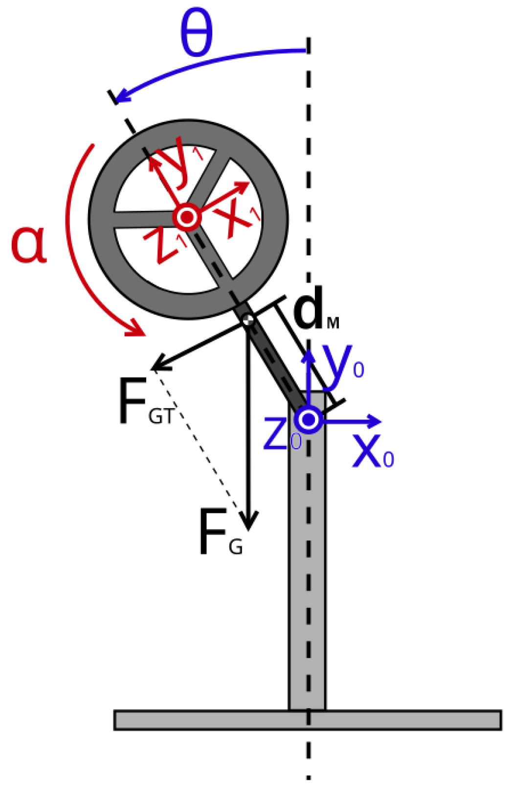
2. Inverted Pendulum Model and Design

2.1. Mathematical Model

In order to analyse the system and design the controller, a mathematical model of a reaction wheel inverted pendulum (RWIP) was first derived. Figure 1 shows the scheme of the RWIP system. It consists of a fixed base, a rotating arm, and a rotating reaction wheel. The frame $(x_0,y_0,z_0)$ is an inertial one and it is related to the pendulum’s base, where $z_0$ represents the axis overlapping the pendulum arm’s axis of rotation. The frame $(x_1,y_1,z_1)$ is a non-inertial frame of the reference related to the end of the moving pendulum’s arm, where $z_1$ is the axis overlapping the wheel’s axis of rotation. The force $F_G$ is the gravitational force acting at the system’s centre of mass. The force $F_{GT}$ is the component of the force $F_G$, perpendicular to the arm of the pendulum. The angle $\theta$ denotes the pendulum’s roll and is measured in the frame $(x_0,y_0,z_0)$ between the vertical, that is, $y_0$, and current position of the pendulum’s arm. It’s acceleration is represented as follows:

$$\ddot{\theta }=\frac{M_p{d}_{M}g}{J}sin\left(\theta \right)-\frac{b_{\theta }}{J}\dot{\theta }+\frac{b_{\alpha }}{J}\dot{\alpha }+\frac{1}{J}{\tau }_d-\frac{1}{J}{\tau }_w,$$

(1)

where $M_p$ is the mass of the pendulum’s arm and reaction wheel combined together; $d_M$ stands for the distance between the axis $z_0$ and the centre of mass; g is the gravity acceleration; J is the pendulum’s total moment of inertia (including the arm, motor, and reaction wheel) with respect to the $z_0$ axis; $b_{\theta }$ and $b_{\alpha }$ are the coefficients of friction associated with angles $\theta$ and $\alpha$, respectively; $\dot{\theta }$ and $\dot{\alpha }$ are first derivatives (angular velocities) of $\theta$ and $\alpha$, respectively; ${\tau }_d$ stands for the torque caused by disturbing forces acting on the pendulum’s arm; and ${\tau }_w$ denotes the torque generated by the reaction wheel. Angle $\alpha$, measured in the frame $(x_1,y_1,z_1)$, describes how much the reaction wheel is rotated around the $z_1$ axis. It denotes acceleration in the frame $(x_0,y_0,z_0)$, which is represented by the following equation:

$$\ddot{\alpha }=-\frac{M_{p}g{d}_M}{J}sin\left(\theta \right)+\frac{b_{\theta }}{J}\dot{\theta }-\frac{(J+J_w)b_{\alpha }}{J{J}_w}\dot{\alpha }-\frac{1}{J}{\tau }_d+\frac{J+J_w}{J{J}_w}{\tau }_w,$$

(2)

where $J_w$ is the wheel’s moment of inertia with respect to the $z_1$ axis.

The reaction wheel is driven by a DC motor, which is described in the following set of equations:

$$\left\{\begin{array}{c}{\tau }_w=k_m{i}_a,\hfill \\ R_a{i}_a+L_a\frac{d{i}_a}{dt}=u-k_e\dot{\alpha },\hfill \end{array}\right.$$

(3)

where u is the motor’s supply voltage, with a maximum value of $U_{dd}=12V$; $i_a$ is the armature circuit current; $R_a$ is the armature circuit resistance; $L_a$ is the armature circuit inductance; $k_m$ is the motor’s mechanical constant; and $k_e$ is the motor’s back electromotive force (EMF) constant.

It was assumed that the time constant of the armature’s circuit is much smaller than the mechanical time constants of the rest of the system. Therefore, $L_a=0$ was assumed. By reformulating Equation (3), the following simplified motor model can be achieved:

$${\tau }_w=\frac{k_m}{R_a}u-\frac{k_m{k}_e}{R_a}\dot{\alpha }.$$

(4)

Introducing (4) into (1) and (2) gives the following combined model of the inverted pendulum:

$$\left\{\begin{array}{c}\ddot{\theta }=\frac{M_p{d}_{M}g}{J}sin\left(\theta \right)-\frac{b_{\theta }}{J}\dot{\theta }+\frac{1}{J}(b_{\alpha }+\frac{k_m{k}_e}{R_a})\dot{\alpha }+\frac{1}{J}{\tau }_d-\frac{1}{J}\frac{k_m}{R_a}u,\hfill \\ \ddot{\alpha }=-\frac{M_{p}g{d}_M}{J}sin\left(\theta \right)+\frac{b_{\theta }}{J}\dot{\theta }-\frac{J+J_w}{J{J}_w}(b_{\alpha }+\frac{k_m{k}_e}{R_a})\dot{\alpha }-\frac{1}{J}{\tau }_d+\frac{J+J_w}{J{J}_w}\frac{k_m}{R_a}u.\hfill \end{array}\right.$$

(5)

Model (5) is a nonlinear one. It is obvious that for small values of $\theta$, $sin\left(\theta \right)=\theta$. Thus, using this property, nonlinear model (5) can be rewritten in a simplified linear form, as follows:

$$\left\{\begin{array}{c}\ddot{\theta }=\frac{M_p{d}_{M}g}{J}\theta -\frac{b_{\theta }}{J}\dot{\theta }+\frac{1}{J}(b_{\alpha }+\frac{k_m{k}_e}{R_a})\dot{\alpha }+\frac{1}{J}{\tau }_d-\frac{1}{J}\frac{k_m}{R_a}u,\hfill \\ \ddot{\alpha }=-\frac{M_{p}g{d}_M}{J}\theta +\frac{b_{\theta }}{J}\dot{\theta }-\frac{J+J_w}{J{J}_w}(b_{\alpha }+\frac{k_m{k}_e}{R_a})\dot{\alpha }-\frac{1}{J}{\tau }_d+\frac{J+J_w}{J{J}_w}\frac{k_m}{R_a}u.\hfill \end{array}\right.$$

(6)

Model (6) can be rewritten in the following equivalent state-space form:

$$\begin{array}{c}\hfill \begin{array}{cc}\hfill \dot{\mathbf{x}}& =\mathbf{A}\mathbf{x}+\mathbf{B}\mathbf{u},\hfill \\ \hfill \mathbf{y}& =\mathbf{C}\mathbf{x},\hfill \end{array}\end{array}$$

(7)

with:

$$\mathbf{x}={\left[\theta \dot{\theta }\alpha \dot{\alpha }\right]}^T,\mathbf{u}={\left[u{\tau }_d\right]}^T,$$

$$\mathbf{A}=\left[\begin{array}{cccc}0& 1& 0& 0\\ \frac{M_p{d}_{M}g}{J}& -\frac{b_{\theta }}{J}& 0& \frac{1}{J}(b_{\alpha }+\frac{k_m{k}_e}{R_a})\\ 0& 0& 0& 1\\ -\frac{M_{p}g{d}_M}{J}& \frac{b_{\theta }}{J}& 0& -\frac{J+J_w}{JJw}(b_{\alpha }+\frac{k_m{k}_e}{R_a})\end{array}\right],\mathbf{B}=\left[\begin{array}{cc}0& 0\\ -\frac{1}{J}\frac{k_m}{Ra}& \frac{1}{J}\\ 0& 0\\ \frac{J+J_w}{JJw}\frac{k_w}{R_a}& -\frac{1}{J}\end{array}\right], \mathbf{C}=\left[\begin{array}{cccc}1& 0& 0& 0\\ 0& 1& 0& 0\\ 0& 0& 1& 0\\ 0& 0& 0& 0\end{array}\right].$$

Variable $\alpha$ does not appear in Equations (5) and (6); therefore, it does not directly affect the dynamics of the system. It can also be observed that $\mathbf{A}$ has a very specific form. However, as can be seen in the matrix $\mathbf{C}$, our physical realisation of the pendulum does not have a sensor that measures the angular velocity of the wheel $\dot{\alpha }$. Thus, its value should be estimated based on measurements of $\alpha$.

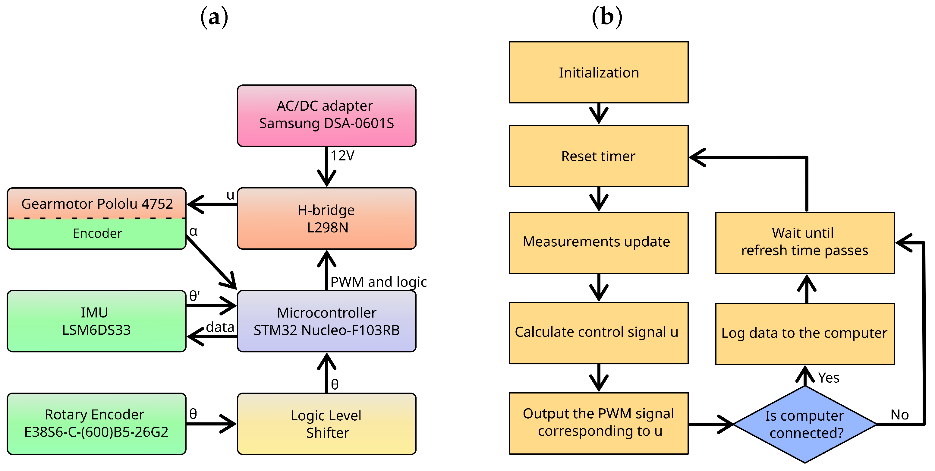
2.2. Physical System Design and Implementation

The pendulum was designed using Fusion 360 software. The final version of the simulation model can be seen in Figure 2a. All of the components were created based on this model. Most of them were cut from wood, but a couple of parts were manufactured using a 3D printer. The complete laboratory stand can be seen in Figure 2b.

The electrical system design boils down to the development of a STM32 Nucleo-F103RB board that acts as a digital controller. It is responsible for collecting data from the following sensors:

• A rotary encoder (E38S6-C-(600)B5-26G2) to measure $\theta$.
• An encoder inside the gear motor (Pololu 4752) to measure $\alpha$.
• An inertial measurement unit (IMU), LSM6DS33, to record $\dot{\theta }$.

The controller stabilises the pendulum by calculating the motor control signal u. It sends a corresponding pulse-width modulation (PWM) signal to the H-bridge module L298N, which feeds the motor. For the sake of simplification, the H-bridge controller is assumed to be a component capable of changing the duty cycle of the PWM signal from 0 to 1 linearly, in a voltage range from 0 to $U_{dd}$, without any losses. The microcontroller unit can operate without the need for external computing systems. It is programmed using the C++ language and uses an internal clock to ensure a constant sampling time. The conceptual component connection diagram is shown in Figure 3a. Moreover, the implementation phases are portrayed in Figure 3b.

3. Parameter Estimation

The following parameters were taken directly from the physical model: $d_M=0.131$ m, $M_p=0.4753$ kg, and $M_w=0.2003$ kg. Other parameters should be derived based on physical laws or should be properly estimated. This process is portrayed in the following sections.

3.1. The Reaction Wheel’s Moment of Inertia

The reaction wheel consists of a wooden disk and weights made of nuts and bolts. The disks mass is $m_d=0.0670$ kg, and the mass of each weight $m_w=0.0333$ kg. The disk was modelled as a uniform annulus with an inner radius $r_i=0.06$ m and an outer radius $r_o=0.10$ m. Its moment of inertia $J_d$ is described by the following formula:

$$J_d=\frac{1}{2}{m}_d(r_i^2+r_o^2)=4.56·{10}^{-4}kg·m^2.$$

(8)

The weights are located at a distance $r_w=0.08$ m from the centre of the annulus. The moment of inertia of the individual weight $J_{iw}$ is approximated by the moment of inertia of a point mass:

$$J_{iw}=m_w{r}_w^2=2.13·{10}^{-4}kg·m^2.$$

(9)

In this way, the moment of inertia of the entire wheel is equal to the following:

$$J_w=J_d+4J_{iw}=1.3·{10}^{-3}kg·m^2.$$

(10)

3.2. The Pendulum’s Moment of Inertia

The moment of inertia J was determined and based on a model of a simple physical pendulum. By knowing the oscillation period T, the moment of inertia can be calculated as follows:

$$J=\frac{T^2}{4{\pi }^2}{M}_{p}g{d}_M.$$

(11)

The reaction wheel was locked, making the pendulum behave like a rigid body, oscillating freely, with a small amplitude. The period of oscillation T was determined by analysing the pendulum’s response, as presented in Figure 4.

$$T=\frac{19.32-0.53}{23}=0.8170s.$$

(12)

Using (11), one can calculate the moment of inertia J as follows:

$$J=0.0103kg·m^2.$$

(13)

3.3. Friction Coefficient

The reaction wheel was kept locked in order to estimate the coefficient of friction $b_{\theta }$. To do this, the pendulum needs to swing faster (with larger $\dot{\theta }$) and thus with a greater amplitude. In this case, the motion of the pendulum, with motion resistance and nonlinear gravity, is described by the following equation:

$$J\ddot{\theta }-M_p{d}_{M}gsin\left(\theta \right)+b_{\theta }\dot{\theta }=0.$$

(14)

Based on (14), a scheme for a nonlinear dynamic model was built in Simulink (see Figure 5). Again, the laboratory stand was forced to swing and measurements of $\theta$ were collected. The obtained measurements were compared with the outputs of the simulation model and the parameter $b_{\theta }$ was adjusted accordingly. The process was repeated to allow us to obtain the lowest value of the mean square error (MSE). In this way, the value of $b_{\theta }=5.6799·{10}^{-6}kg{m}^2{s}^{-1}$ was estimated.

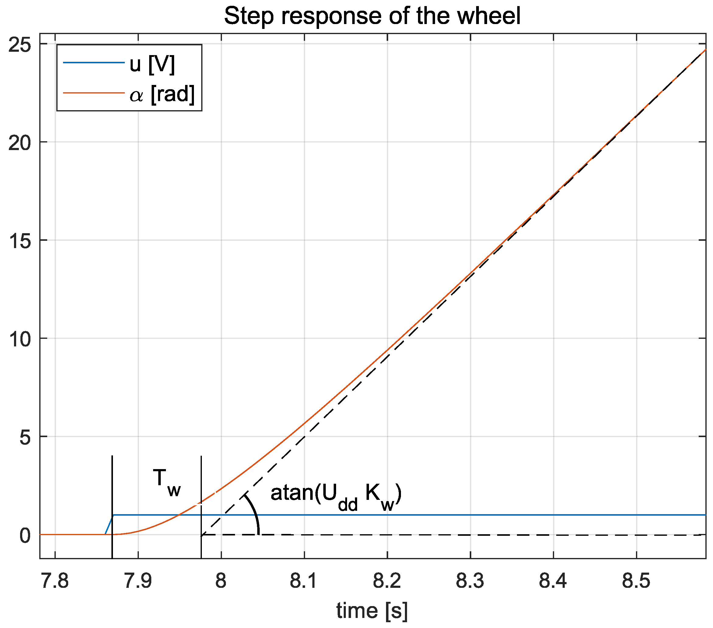
3.4. The Motor’s Parameters

In order to determine the parameters of the motor, the pendulum’s arm was kept fixed ($\theta =\mathbf{const}$). In this case, the reaction wheel accelerates according to the following equation:

$$J_w\ddot{\alpha }+\left(b_{\alpha }+\frac{k_m{k}_e}{R_a}\right)\dot{\alpha }=\frac{k_m}{R_a}u.$$

(15)

Let $T_w=J_w{(b_{\alpha }+\frac{k_m{k}_e}{R_a})}^{-1}$ and $K_w={(b_{\alpha }+\frac{k_m{k}_e}{R_a})}^{-1}\frac{k_m}{R_a}$. Then, (15) can be rewritten into the following form:

$$T_w\ddot{\alpha }+\dot{\alpha }=K_{w}u.$$

(16)

The time constant $T_w$ and gain $K_w$ were estimated based on the step response of the motor, as illustrated in Figure 6.

From the step response shown in Figure 6, the value of $T_w$ was found to be equal to $0.1s$, while $K_w$ was derived based on the slope of the step response; its value is equal to $3.4114V^{-1}{s}^{-1}$. The rest of parameters were derived from (15) as follows:

$$\begin{array}{cc}\hfill (b_{\alpha }+\frac{k_m{k}_e}{R_a})& =\frac{J_w}{T_w}=0.0131,\hfill \\ \hfill \frac{k_m}{R_a}& =K_w(b_{\alpha }+\frac{k_m{k}_e}{R_a})=0.0447.\hfill \end{array}$$

(17)

3.5. Summary of the Model’s Parameters

All the necessary parameters concerning successful system modelling are summarised in

Table 1. List of all the parameters needed for system modelling.

Parameter	Value	Unit
$d_M$	$0.131$	m
$M_p$	$0.4753$	kg
$M_w$	$0.2003$	kg
J	$0.0103$	$kg{m}^2$
$J_w$	$0.0013$	$kg{m}^2$
$b_{\theta }$	$5.6799·{10}^{-6}$	$kg{m}^2{s}^{-1}$
$(b_{\alpha }+\frac{k_m{k}_e}{R_a})$	$0.0131$	$kg{m}^2{s}^{-1}$
$\frac{k_m}{R_a}$	$0.0447$	$kg{m}^2{s}^{-2}{V}^{-1}$
g	$9.81$	$m{s}^{-2}$

. A final comparison between the derived model and the laboratory stand can be seen in Figure 7. This comparison presents the rectangular pulse response of the considered pendulum system.

4. Control of Inverted Pendulum

In order to control RWIP, two closed-loop method were examined and compared: a cascade control system with two PID controllers and a linear–quadratic–Gaussian (LQG) control system.

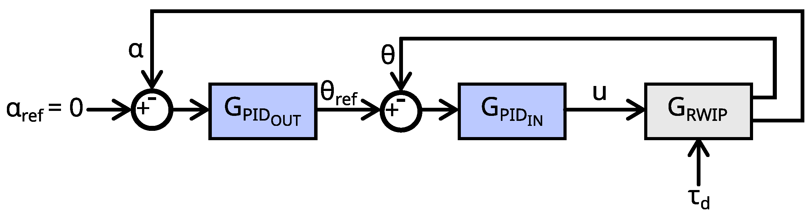
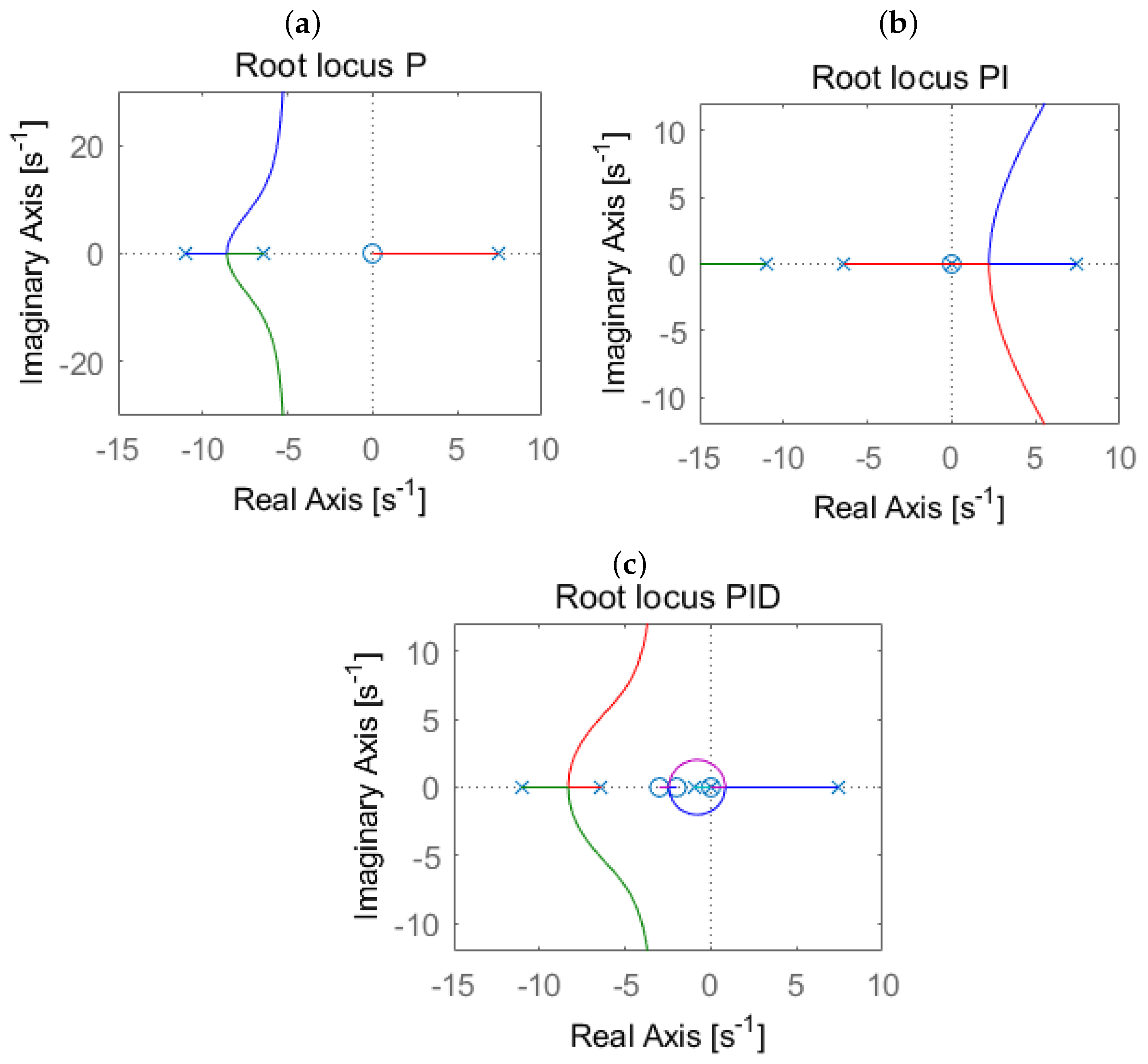
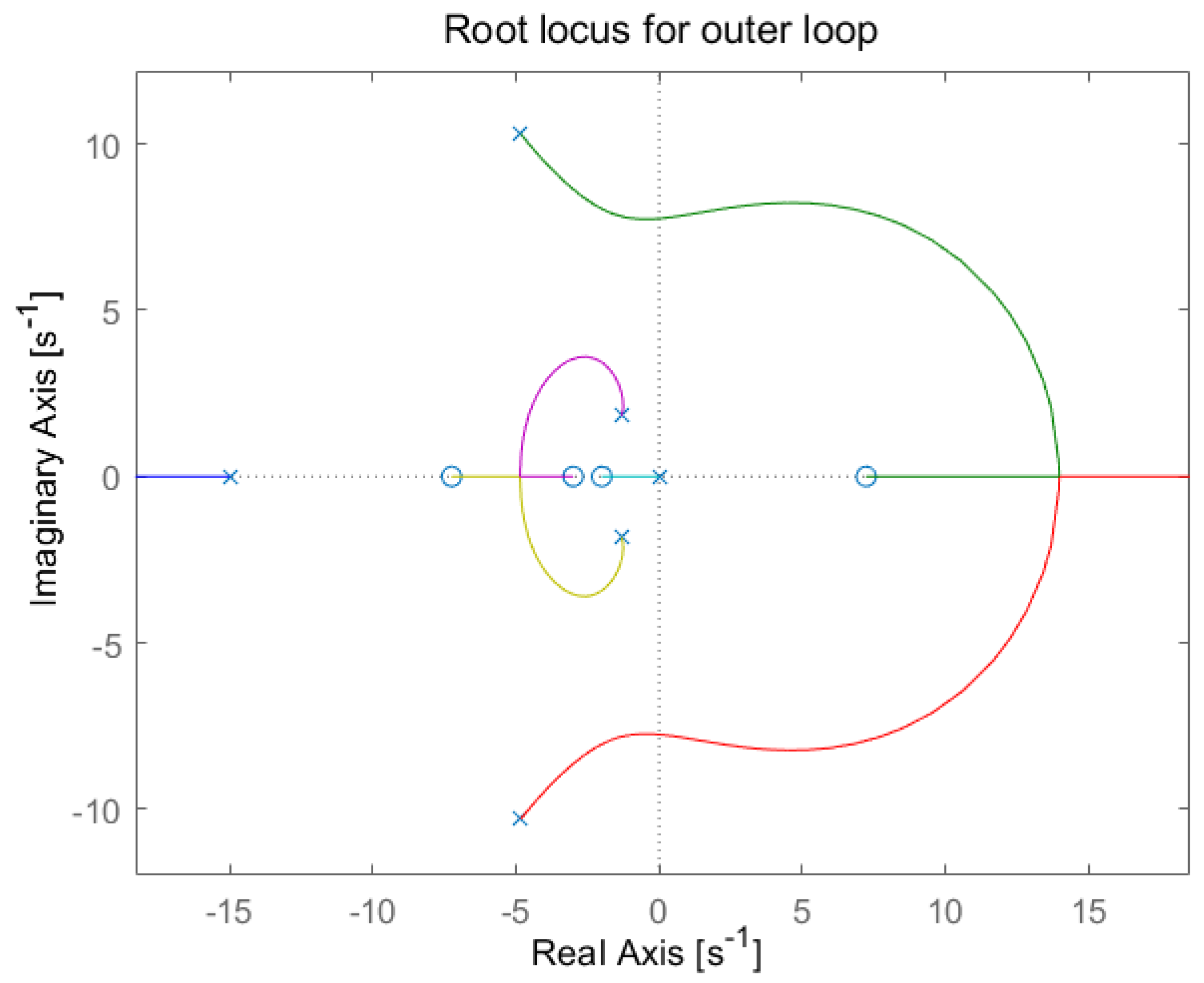
4.1. Cascade PID Control

As an input, the PID controller is fed with an error signal, which is the difference between the reference of the measured output, i.e., $e=y_{ref}-y$. Based on this error, a control signal is generated that affects the system in such a way as to minimise it. For an ideal PID controller, the control signal is proportional to the current difference $K_p$ (P term), the integral of the previous error values $K_i\frac{1}{s}$ (I term), and the error rate of change $K_{d}s$ (D term). In practice, the differentiating component amplifies the high-frequency signals, including noise, and oscillations caused by the step changes of the digital signal. To avoid this, a low-pass filter is added, resulting in a filtered version of the PID controller, as follows:

$$G_{PIDF}\left(s\right)=K_p+\frac{K_i}{s}+\frac{K_{d}s}{T_{f}s+1},$$

(18)

where $T_f$ is the time constant of the low-pass filter. This form was implemented within the microcontroller. However, for design purposes, a representation that exhibits the positions of the controller’s zeros and poles was employed, as follows:

$$G_{PIDF}\left(s\right)=K_m\frac{(s-s_{z1})(s-s_{z2})}{s(s-s_p)},$$

(19)

where $s_{z1}$ and $s_{z2}$ represent zeros, $s_p$ denotes the pole, and $K_m$ is the overall gain of the controller. Subsequently, it is possible to transition from notation (19) to (18) using the following substitutions:

$$\begin{array}{cc}\hfill K_p& =K_m[(s_{z1}+s_{z2})s_p-2s_{z1}{s}_{z2}]s_p^{-2},\hfill \\ \hfill K_i& =-K_m{s}_{z1}{s}_{z2}{s}_p^{-1},\hfill \\ \hfill K_d& =-K_m{s}_p^{-1}+K_m[(s_{z1}+s_{z2})s_p-s_{z1}{s}_{z2}]s_p^{-3},\hfill \\ \hfill T_f& =-s_p^{-1}.\hfill \end{array}$$

(20)

For the remainder of the paper, the name PID is used to denote the filtered version.

The cascade structure of the control system, shown in Figure 8, was used to stabilise the pendulum. It consists of an inner loop with a controller, represented by the transfer function $G_{PI{D}_{in}}\left(s\right)$, and an outer loop with the controller $G_{PI{D}_{out}}\left(s\right)$. The transfer function of the pendulum is denoted by $G_{RWIP}\left(s\right)$. The task of the inner control loop is to quickly stabilise $\theta$. The outer loop stabilises the variable $\alpha$ by providing the reference signal ${\theta }_{ref}$ for the inner control loop. Because of the derivative term in $G_{PI{D}_{out}}$, if the velocity $\dot{\alpha }$ increases, then ${\theta }_{ref}$ decreases. This forces the pendulum to tilt slightly in the opposite direction. To maintain stability, the wheel begins to accelerate in the opposite direction. As a result, the velocity $\dot{\alpha }$ decreases, and ${\theta }_{ref}$ and $\theta$ go back to zero.

Note that both controllers were designed based on the root locus method. As shown in Figure 9, using state-space representation (7), the pole–zero maps of the pendulum were derived with respect to the input signal u.

The system has an unstable pole at $s=7.439$. In addition, in the transfer function representing the output $\alpha$, there is a right-half-plane zero at $s=7.25$, which creates a non-minimum-phase system. It should be also mentioned that by taking into account the $\theta$ output, the system has one zero at the origin. Moreover, by taking $\dot{\theta }$ into account, it is evident that there are two zeros at the origin.

Let us analyse the root locus of the inner loop. Using the proportional term of $G_{PI{D}_{in}}$ alone, the unstable pole tends towards zero at the origin of the complex plane. This feature is illustrated in Figure 10a. As a result, the P controller itself is not able to stabilise the system. An additional pole is therefore added at the origin. The system is still unstable; however, the unstable pole is now no longer attracted to the origin (see Figure 10b). Finally, additional zeros and a pole were added at $s_{z1}=-3$, $s_{z2}=-2$, and $s_p=-1$. As portrayed in Figure 10c, this forces the unstable pole to attract $s_{z2}$.

The gain was chosen so that the unstable pole is moved to the left half-plane and the dominant poles provide an overshoot of around $12\%$ for $K_m=-4$. The negative gain is due to the opposite directions in which the reaction wheel and the pendulum arm rotate. This can be seen in matrix $\mathbf{B}$—from input u to $\dot{\theta }$, there is a negative coefficient, while there is a positive one up to $\dot{\alpha }$. The purpose of the inner loop is to control $\theta$ and, hence, a negative gain is needed. By applying the pole and zeros’ locations to (19) and using (20), the transmittance of the inner controller in the parallel form (18) is obtained as follows:

$$G_{PI{D}_{in}}=-4\frac{(s+3)(s+2)}{s(s+1)}=4-\frac{24}{s}-\frac{8s}{s+1},$$

(21)

where $K_p=4$, $K_i=-24$, $K_d=-8$, and $T_f=1$. Such settings make it possible to stabilise $\theta$ to the required reference level. Figure 11 shows the root locus for the outer loop, which is based on the inner loop. A pole in the origin indicates the presence of an integral component. For that reason, an additional integral component would make the regulation worse. Therefore, the structure of the outer controller was simplified to include only the proportional and derivative components. The root locus plot gain was set to $K_m=0.01$ and the transfer function of $G_{PI{D}_{out}}$ was chosen as follows:

$$G_{P{D}_{out}}=0.01\frac{s}{s+15}=\frac{0.000667s}{0.0667s+1},$$

(22)

with $K_p=0$, $K_i=0$, $K_d=0.000667$, and $T_f=0.0667$.

Figure 12 shows the simulated step responses of the pendulum with respect to u and ${\tau }_d$. The system is stable in the bounded-input, bounded-output (BIBO) sense, taking into account the step response for signal u (the left part of Figure 12). However, it is not fully stable for the input ${\tau }_d$ (the right part of Figure 12). This can be clearly seen in the response of signal $\alpha$. It was not considered to be a major problem because signal $\alpha$ is not the control target. However, it introduces a non-zero constant velocity $\dot{\alpha }$, which, in practice—with a large ${\tau }_d$—may saturate the motor and destabilise the pendulum.

4.2. Linear–Quadratic–Gaussian Controller

Alternatively, a state-feedback-based controller was designed. This control scheme is based on full information about the system state $\mathbf{x}$. If it is not fully available, a state observer is created to provide its estimate $\widehat{\mathbf{x}}$. The state feedback makes it possible to shift the poles of the closed-loop system to any position in the complex plane [18]. Such a design method is very desirable and is suitable for dealing with multiple-input and multiple-output (MIMO) systems. One important characteristic is that it is able to handle dynamic coupling between state variables. LQG combines such an LQR controller with a Kalman filter as a state estimator. According to the separation principle [19], the design process of the controller and the state estimator can be split without exerting a negative influence on the control performance.

The controller design was realised using a microcontroller, which is a digital device. Therefore, the state-space model (7) was discretised. For that purpose, the zero-order hold method was employed. Moreover, the refreshing time of the microcontroler was set to 12 ms. Finally, the discrete-time state-space model of the open-loop system has the following form:

$$\begin{array}{cc}\hfill \mathbf{x}[k+1]& ={\mathbf{A}}_{\mathbf{d}}\mathbf{x}\left[k\right]+{\mathbf{B}}_{\mathbf{d}}\mathbf{u}\left[k\right],\hfill \end{array}$$

(23)

$$\begin{array}{cc}\hfill \mathbf{y}\left[k\right]& ={\mathbf{C}}_{\mathbf{d}}\mathbf{x}\left[k\right],\hfill \end{array}$$

(24)

where

$${\mathbf{A}}_{\mathbf{d}}=\left[\begin{array}{cccc}1.0042& 0.0120& 0& 0.0001\\ 0.7056& 1.0042& 0& 0.0142\\ -0.0041& -0.0000& 1.0000& 0.0112\\ -0.6649& -0.0041& 0& 0.8735\end{array}\right],$$

$${\mathbf{B}}_{\mathbf{d}}=\left[\begin{array}{cc}-0.0036& 0.0069\\ -0.5832& 1.1552\\ 0.0318& -0.0067\\ 5.1780& -1.0884\end{array}\right],{\mathbf{C}}_{\mathbf{d}}=\left[\begin{array}{cccc}1& 0& 0& 0\\ 0& 1& 0& 0\\ 0& 0& 1& 0\\ 0& 0& 0& 0\end{array}\right].$$

It should be kept in mind that the second column of the matrix ${\mathbf{B}}_{\mathbf{d}}$ is related to the distortion input ${\tau }_d$ and cannot be used to control the system. This means that its effect should be decoupled while estimating an unknown state $\mathbf{x}\left[k\right]$. To settle this problem, a Kalman filter with an unknown input is employed [20]. In particular, the matrix ${\mathbf{B}}_{\mathbf{d}}$ is split into two components, ${\mathbf{B}}_{\mathbf{dc}}$ and ${\mathbf{B}}_{ø}$. They correspond to the first and second columns of ${\mathbf{B}}_{\mathbf{d}}$. As indicated in [20], the primary design condition underlying the unknown input Kalman filter is

$$\mathrm{rank}\left({\mathbf{C}}_{\mathbf{d}}{\mathbf{B}}_{ø}\right)=\dim {\tau }_d=1,$$

(25)

which is clearly satisfied. Finally, the unknown input Kalman filter is given by the following:

$$\begin{array}{cc}\hfill \widehat{\mathbf{x}}[k/k-1]& ={\mathbf{A}}_{\mathbf{d}}\widehat{\mathbf{x}}[k-1/k-1]+{\mathbf{B}}_{\mathbf{dc}}\mathbf{u}[1,k-1],\hfill \end{array}$$

(26)

$$\begin{array}{cc}\hfill \widehat{\tau }[d,k-1]& =\mathbf{M}(\mathbf{y}\left[k\right]-{\mathbf{C}}_{\mathbf{d}}\widehat{\mathbf{x}}[k/k-1]),\hfill \end{array}$$

(27)

$$\begin{array}{cc}\hfill {\widehat{\mathbf{x}}}^{*}[k/k]& =\widehat{\mathbf{x}}[k/k-1]+{\mathbf{B}}_{ø}\widehat{\tau }[d,k-1],\hfill \end{array}$$

(28)

$$\begin{array}{cc}\hfill \widehat{\mathbf{x}}[k/k]& ={\widehat{\mathbf{x}}}^{*}[k/k]+{\mathbf{K}}_{\mathbf{k}}(\mathbf{y}\left[k\right]-{\mathbf{C}}_{\mathbf{d}}{\widehat{\mathbf{x}}}^{*}[k/k])\hfill \end{array}$$

(29)

where the matrix $\mathbf{M}={\left({\mathbf{C}}_{\mathbf{d}}{\mathbf{B}}_{ø}\right)}^{+}$, with ${(·)}^{+}$ being a pseudo-inverse of its argument. Finally, the Kalman filter gain matrix is calculated according to the strategy proposed in [20].

The scheme of the closed system with state feedback and the Kalman filter is shown in Figure 13, with ${\mathbf{K}}_{\mathbf{lqr}}$ denoting the optimal feedback gain matrix.

4.2.1. Feedback Gain

When designing a control system, it should be ensured that the system is controllable. The rank of the controllability matrix $\mathbf{T}$ is equal to the rank of the state vector

$$rank\left(\mathbf{T}\right)=rank\left(\left[{\mathbf{B}}_{\mathbf{dc}}{\mathbf{A}}_{\mathbf{d}}{\mathbf{B}}_{\mathbf{dc}}{\mathbf{A}}_{\mathbf{d}}^{\mathbf{2}}{\mathbf{B}}_{\mathbf{dc}}{\mathbf{A}}_{\mathbf{d}}^{\mathbf{3}}{\mathbf{B}}_{\mathbf{dc}}\right]\right)=4,$$

which means that the pendulum is controllable.

In order to calculate the feedback gain ${\mathbf{K}}_{\mathbf{lqr}}$, the state-cost weighted matrix ${\mathbf{Q}}_{\mathbf{lqr}}$ and the input-cost weighted matrix ${\mathbf{R}}_{\mathbf{lqr}}$ were defined. The values of the ${\mathbf{Q}}_{\mathbf{lqr}}$ matrix were adjusted to prioritise the stabilisation of angle $\theta$ more than $\alpha$. Then, based on the simulations carried out, the value of ${\mathbf{R}}_{\mathbf{lqr}}$ was selected so that u was between -$U_{dd}$ and $U_{dd}$ for the desired degree of stabilisation.

$${\mathbf{Q}}_{\mathbf{lqr}}=\left[\begin{array}{cccc}10& 0& 0& 0\\ 0& 10& 0& 0\\ 0& 0& 0.1& 0\\ 0& 0& 0& 0.1\end{array}\right]$$

(30)

$${\mathbf{R}}_{\mathbf{lqr}}=2$$

(31)

Finally, the optimal gain ${\mathbf{K}}_{\mathbf{lqr}}$ aims to minimise the quadratic cost function $J_d$, defined as follows:

$$J_d\left(u\right)=\sum _{n=1}^{\infty }(\mathbf{x}{\left[k\right]}^T{\mathbf{Q}}_{\mathbf{lqr}}\mathbf{x}\left[k\right]+\mathbf{u}{\left[k\right]}^T{\mathbf{R}}_{\mathbf{lqr}}\mathbf{u}\left[k\right]).$$

(32)

with the control law $\mathbf{u}\left[k\right]=-{\mathbf{K}}_{\mathbf{lqr}}\mathbf{x}\left[k\right]$. This yields the following:

$${\mathbf{K}}_{\mathbf{lqr}}=[-18.2432-2.6777-0.0966-0.1529].$$

(33)

After closing the feedback loop, the discrete closed-loop system is described by the following equation:

$$\begin{array}{cc}\hfill \mathbf{x}[k+1]& =({\mathbf{A}}_{\mathbf{d}}-{\mathbf{B}}_{\mathbf{dc}}{\mathbf{K}}_{\mathbf{lqr}})\mathbf{x}\left[k\right]+{\mathbf{B}}_{\mathbf{d}}\mathbf{u}\left[k\right],\hfill \end{array}$$

(34)

$$\begin{array}{cc}\hfill \mathbf{y}\left[k\right]& ={\mathbf{C}}_{\mathbf{d}}\mathbf{x}\left[k\right].\hfill \end{array}$$

(35)

The poles’ locations are included in $\mathbf{poles}=[-0.1167+0.0000i,0.9370+0.0272i,0.9370-0.0272i,0.9881+0.0000i]$ with the following magnitudes: $\left|\mathbf{poles}\right|=[0.1167,0.9374,0.9374,0.9881]$. Clearly, all poles are located inside the unit circle, which means that state feedback successfully stabilises the model. The system’s step responses are shown in Figure 14. In contrast to the cascade PID controller, this time, the velocity $\dot{\alpha }$ converges to zero. For this reason, the motor is not saturated in a steady state.

4.2.2. State Observer

The state estimator aims at reconstructing the current state of the system based on the measurements and a mathematical model of the system. In this case, this mainly refers to the estimation of $\dot{\alpha }$. However, a Kalman filter is used as a full-state observer; thus, other state variable estimates were also obtained.

First, it was verified whether the system is observable or not. The rank of the observability matrix $\mathbf{O}$ is equal to the dimension of the state vector

$$rank\left(\mathbf{O}\right)=rank\left(\left[{\mathbf{C}}_{\mathbf{d}}{\mathbf{C}}_{\mathbf{d}}{\mathbf{A}}_{\mathbf{d}}{\mathbf{C}}_{\mathbf{d}}{\mathbf{A}}_{\mathbf{d}}^{\mathbf{2}}{\mathbf{C}}_{\mathbf{d}}{\mathbf{A}}_{\mathbf{d}}^{\mathbf{3}}\right]\right)=4,$$

which means that the system is observable.

The estimator is based on a linear model (6), and it is itself a dynamic system, which can be described by the following equation:

$$\begin{array}{cc}\hfill \widehat{\mathbf{x}}[k+1]& =({\mathbf{A}}_{\mathbf{d}}-{\mathbf{B}}_{\mathbf{dc}}{\mathbf{K}}_{\mathbf{lqr}})\widehat{\mathbf{x}}\left[k\right]+{\mathbf{B}}_{\mathbf{d}}\mathbf{u}\left[k\right]+{\mathbf{K}}_{\mathbf{kf}}(\mathbf{y}\left[k\right]-\widehat{\mathbf{y}}\left[k\right]),\hfill \\ \hfill \widehat{\mathbf{y}}\left[k\right]& ={\mathbf{C}}_{\mathbf{d}}\widehat{\mathbf{x}}\left[k\right].\hfill \end{array}$$

(36)

where $\widehat{\mathbf{x}}\left[k\right]$ is the estimate of the system’s state at time k, while $\widehat{\mathbf{y}}\left[k\right]$ is the estimate of the system’s output at time k.

The covariance of the process noise ${\mathbf{Q}}_{\mathbf{kf}}$ and the measurement noise ${\mathbf{R}}_{\mathbf{kf}}$ was assumed to be constant and have the following form:

$$\begin{array}{cc}\hfill {\mathbf{Q}}_{\mathbf{kf}}& =\left[\begin{array}{cc}{10}^{-1}& 0\\ 0& {10}^0\end{array}\right],\hfill \\ \hfill {\mathbf{R}}_{\mathbf{kf}}& =\left[\begin{array}{cccc}2·{10}^{-3}& 0& 0& 0\\ 0& 5·{10}^1& 0& 0\\ 0& 0& 1·{10}^{-1}& 0\\ 0& 0& 0& {10}^{10}\end{array}\right].\hfill \end{array}$$

(37)

It was assumed that both the measurement and the process noise are uncorrelated. This assumption leads to the diagonal form of covariance matrices. The covariance of the measurement noise was selected based on an analysis of the recorded data. In turn, the covariance of the process noise was selected via a trial and error method. Such settings guarantee a good unknown input Kalman filter performance for the whole operational range of the inverted pendulum.

4.3. Comparative Evaluation

In order to compare the control systems based on PID and LQR controllers, four performance indices were considered:

• The maximum absolute value of the controlled signal $x_{max}$.
• The settling time $t_r$, calculated as the time from the moment the system is excited until the signal error $e_x\left(t\right)=x\left(t\right)-x_{final}$ reaches and remains constantly within the tolerance zone $\pm 0.05·e_{max}$, with $e_{max}$ being the maximum error.
• The percentage overshoot $P{O}_0$—calculated for signals with a zero steady-state value as the ratio of two adjacent peak amplitudes: $P{O}_0=x_{peak1}/x_{peak2}·100\%$.
• The percentage overshoot $P{O}_n$—calculated for signals with a non-zero steady-state value: $P{O}_n=(x_{peak1}-x_{final})/x_{final}·100\%$.

The quantitative control indices are listed in

Table 2. Performance indices for cascade PID and LQR controllers.

	Cascade PID
	Input $\mathit{u}$			Disturbance ${\mathit{\tau }}_{\mathit{d}}$
Variable	$\theta$	$\alpha$	$\dot{\alpha }$	$\theta$	$\alpha$	$\dot{\alpha }$
$x_{max}$	$0.0073rad$	$1rad$	$1.14\frac{rad}{s}$	$0.033rad$	–	$40\frac{rad}{s}$
$t_r$ [s]	$1.72$	$5.52$	$3.95$	$6.3$	–	7
$P{O}_0[\%]$	28	–	–	–	–	–
$P{O}_n[\%]$	–	0	–	0	–	0
	LQR
	Input u			Disturbance ${\tau }_d$
Variable	$\theta$	$\alpha$	$\dot{\alpha }$	$\theta$	$\alpha$	$\dot{\alpha }$
$x_{max}$	$0.033rad$	$7.6rad$	$5.55\frac{rad}{s}$	$1.93rad$	$302rad$	$215\frac{rad}{s}$
$t_r$ [s]	$2.6$	$3.28$	$3.6$	$2.1$	$3.2$	$3.6$
$P{O}_0[\%]$	22	–	–	–	–	–
$P{O}_n[\%]$	–	0	–	$18.3$	0	–

.

Clearly, the cascade PID controller achieves smaller $x_{max}$ values than the LQR controller. In the case of the control input, the regulation time of $\theta$ is better for the cascade PID controller, but the overshoot is slightly lower for the LQR controller. In the case of the disturbance ${\tau }_d$, the LQR controller performs better than the PID controller. Obviously, the cascade PID has problems—with a proper control of $\alpha$, one could not provide the quality indices in that case. Taking into account all performance indices as well as disturbance compensation abilities, it can be concluded that the LQR controller performs better than the cascade PID controller.

5. Experimental Results

The designed and investigated control systems were tested in two ways: (i) under undisturbed operating conditions and (ii) with a constant disturbance force caused by additional weights. Both video recordings of the experiments and data collected are portrayed in the following subsections.

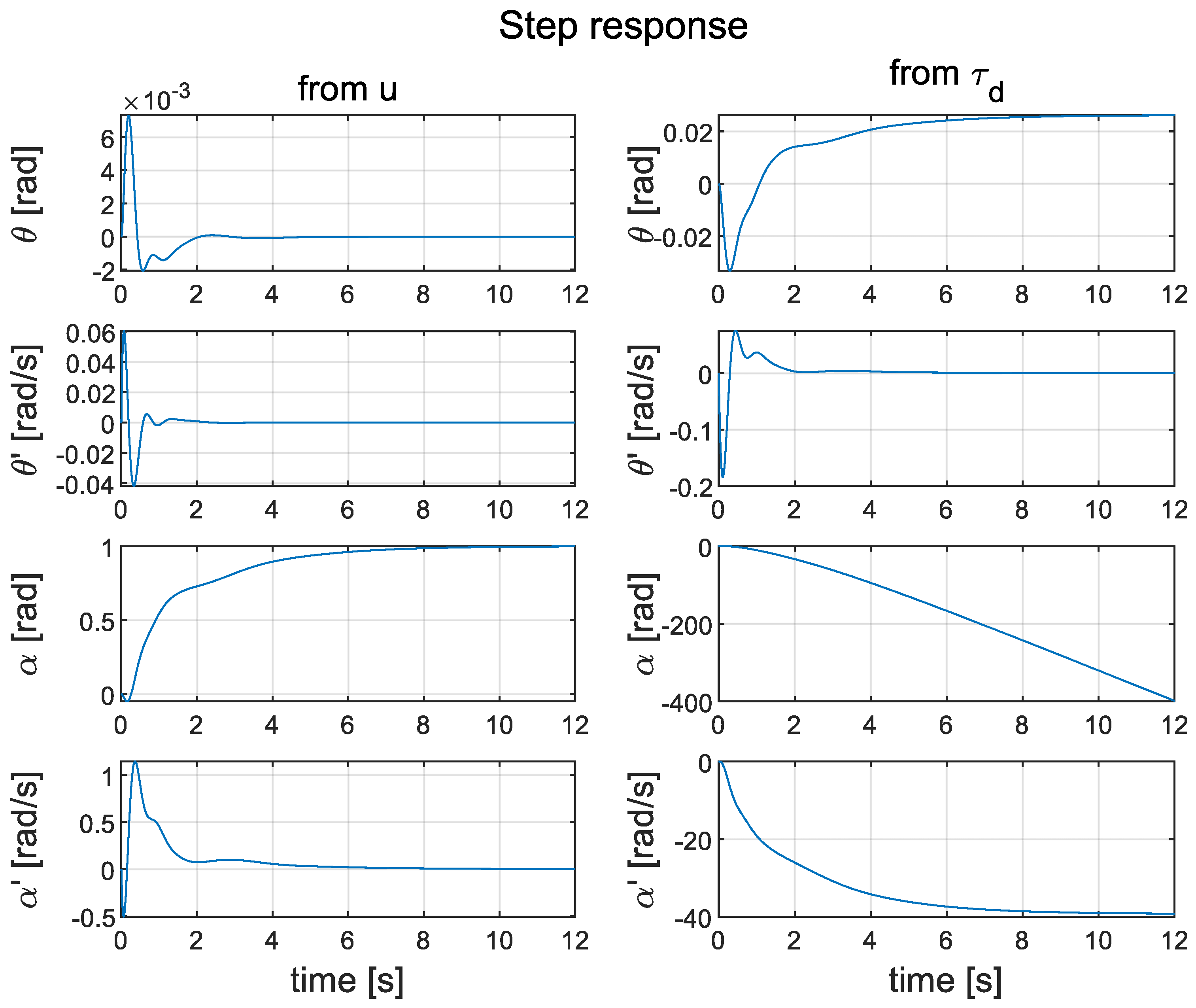
5.1. Impulse Disturbance Torque

Both control systems were tested at the under normal operating conditions. Additionally, in the steady state, the pendulum was lightly pushed with a wooden bar.

The cascade PID controller was able to stabilise the system. Interested readers can find a video of the controller’s performance on the following webpage: https://www.youtube.com/shorts/TG2SWD9OdJk. However, this method results in a non-zero reaction wheel speed ($\dot{\alpha }\ne 0$). This can be seen in Figure 15. It can also be observed that the control signal u is very noisy.

The LQG controller also successfully stabilised the pendulum. For a video of the controller’s performance, please visit the following webpage: https://youtube.com/shorts/Kn4MKzpV6JI. The system balances around its equilibrium point with the speed of the wheel $\dot{\alpha }$ oscillating around 0 rad/s. The control signal u is much less noisy than in the case of the cascade controller.

Both systems were able to function properly following a light push of the bar, but the LQG controller was much more robust. The results presented in Figure 15 include the response of the pendulum to pushes occurring at the time instants $t=63.6$ s and $t=64.2$ s, while Figure 16 presents the response of the pendulum when the bar was pushed at $t=146.5$ s, $t=149.4$ s, and $t=153.2$ s.

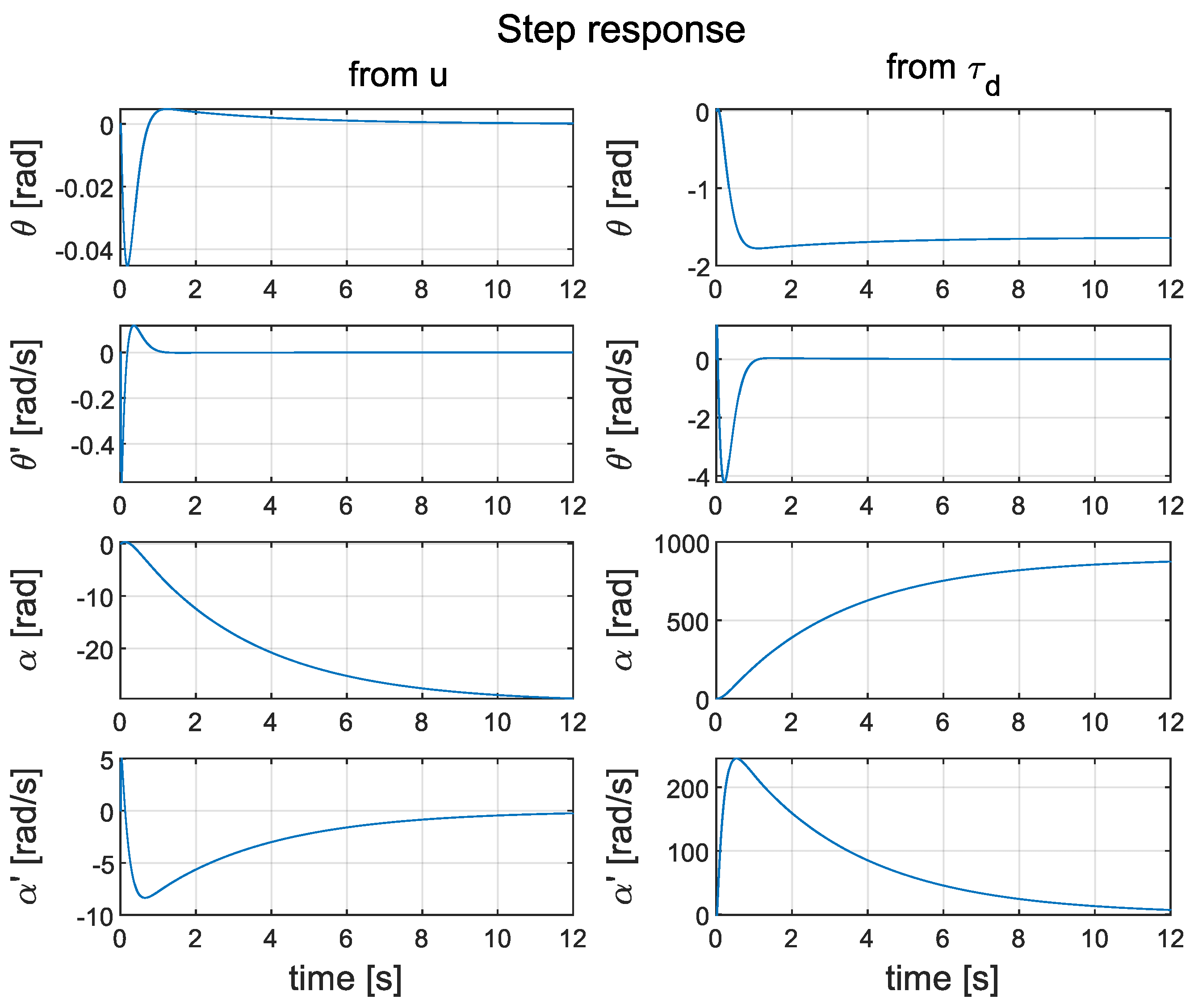
5.2. Constant Disturbance Torque

As part of this experiment, an arm was attached to the pendulum. Weights of 35 g each were added to the pendulum in a stepwise manner. The system recognises these weights as step changes in the disturbance torque signal ${\tau }_d$. A video showing the performance of the pendulum in the case of the cascade controller can be found at https://www.youtube.com/shorts/pgWTVsNW0Pg; a video showing the LQR controller can be found at https://youtu.be/yshctkoC1pk. A portion of the measured data for the cascade structure is shown in Figure 17; data for the LQR controller can be found in Figure 18. The closed-loop system with the LQR controller can handle additional weights very well. On the other hand, adding weights to the cascade design increases the average wheel speed $\dot{\alpha }$ during steady-state operation. It saturates the motor very quickly, which causes the pendulum to lose stability. It should be noted that the control signal u in the case of the LQR controller is, again, smoother than that in the cascade control system.

A constant, non-zero value of torque disturbance ${\tau }_d$ contributes a constant static error of $\theta$. This is true for both the cascade and LQR controllers. This appear to degrade the performance of the control system. However, it can be a desirable property. A constant ${\tau }_d$ shifts the equilibrium point of the pendulum. The LQR controller brings $\theta$ to such a position that the torque created by the gravity force neutralises the influence of the constant ${\tau }_d$.

6. Conclusions

In this study, the development of a mathematical model of a pendulum with a reaction wheel was described. Based on this, a physical inverted pendulum system was designed and successfully implemented. For this purpose, the appropriate sensors, motor, and microcontroller were selected. The linearised pendulum model was implemented in the Matlab environment. Based on this, cascade PID and LQG controllers were developed. Finally, they were implemented in the physical pendulum system. In order to collect the measurements, a connection was established between the microcontroller and a personal computer. The estimation of the model parameters was based on the knowledge acquired from the basic physical relations. This proved to be sufficient for developing a good mathematical model. Finally, the stabilisation of the RWIP was also successful. Both the cascade PID and LQG controllers were able to stabilise the pendulum. Using the cascade controller, the pendulum balanced at approximately $\pm 0.01$ rad around the equilibrium point, while the LQG controller balanced at approximately $\pm 0.025$ rad. However, it was evident that the LQG controller was able to deal much better with noise and disturbances. Moreover, the design process of the LQG controller was much easier than the cascade PID controller. The application of state feedback made it straightforward to move the poles of the device. Because of the coupling between $\theta$ and $\alpha$, designing a cascade controller was more difficult.

Note that the main limitation of this approach was eliminated by applying an unknown input Kalman filter, which served as a torque disturbance estimator, thereby enabling greater robustness to external disturbances.

Motivated by these promising results with the LQG approach, further research will be oriented towards:

• Investigating the selection of the Kalman filter covariance matrices in order to better deal with both changing noise and disturbances.
• Relaxing the small-angle assumption and deriving a linear parameter-varying (LPV) model of the pendulum.
• Designing LPV controllers and state observers.

References

1. Aranovskiy, S.; Biryuk, A.; Nikulchev, E.V.; Ryadchikov, I.; Sokolov, D. Observer design for an inverted pendulum with biased position sensors. J. Comput. Syst. Sci. Int. 2019, 58, 297–304. [Google Scholar] [CrossRef]
2. Xu, Q.; Stepan, G.; Wang, Z. Balancing a wheeled inverted pendulum with a single accelerometer in the presence of time delay. J. Vib. Control 2017, 23, 604–614. [Google Scholar] [CrossRef]
3. Hamza, M.F.; Yap, H.J.; Choudhury, I.A.; Isa, A.I.; Zimit, A.Y.; Kumbasar, T. Current development on using Rotary Inverted Pendulum as a benchmark for testing linear and nonlinear control algorithms. Mech. Syst. Signal Process. 2019, 116, 347–369. [Google Scholar] [CrossRef]
4. Mehedi, I.M.; Ansari, U.; Al-Saggaf, U.M. Three degrees of freedom rotary double inverted pendulum stabilization by using robust generalized dynamic inversion control: Design and experiments. J. Vib. Control. 2020, 26, 2174–2184. [Google Scholar] [CrossRef]
5. Baimukashev, D.; Sandibay, N.; Rakhim, B.; Varol, H.A.; Rubagotti, M. Deep learning-based approximate optimal control of a reaction-wheel-actuated spherical inverted pendulum. In Proceedings of the 2020 IEEE/ASME International Conference on Advanced Intelligent Mechatronics (AIM), Boston, MA, USA, 6–9 July 2020; pp. 1322–1328. [Google Scholar]
6. Du, D.; Zhang, C.; Song, Y.; Zhou, H.; Li, X.; Fei, M.; Li, W. Real-time Hinf control of networked inverted pendulum visual servo systems. IEEE Trans. Cybern. 2019, 50, 5113–5126. [Google Scholar] [CrossRef] [PubMed]
7. Bezci, Y.E.; Aghaei, V.T.; Akbulut, B.E.; Tan, D.; Allahviranloo, T.; Fernandez-Gamiz, U.; Noeiaghdam, S. Classical and intelligent methods in model extraction and stabilization of a dual-axis reaction wheel pendulum: A comparative study. Results Eng. 2022, 16, 100685. [Google Scholar] [CrossRef]
8. Nguyen, B.H.; Cu, M.P.; Nguyen, M.T.; Tran, M.S.; Tran, H.C. Lqr and fuzzy control for reaction wheel inverted pendulum model. Robot. Manag. 2019, 24. [Google Scholar]
9. Trentin, J.F.S.; Da Silva, S.; Ribeiro, J.M.D.S.; Schaub, H. Inverted pendulum nonlinear controllers using two reaction wheels: Design and implementation. IEEE Access 2020, 8, 74922–74932. [Google Scholar] [CrossRef]
10. Belascuen, G.; Aguilar, N. Design, modeling and control of a reaction wheel balanced inverted pendulum. In Proceedings of the 2018 IEEE Biennial Congress of Argentina (ARGENCON), San Miguel de Tucuman, Argentina, 6–8 June 2018; pp. 1–9. [Google Scholar]
11. Önen, Ü.; Çakan, A. Multibody modeling and balance control of a reaction wheel inverted pendulum using lqr controller. Int. J. Robot. Control Syst. 2021, 1, 84–89. [Google Scholar] [CrossRef]
12. Chinelato, C.I.G.; Neves, G.P.D.; Angélico, B.A. Safe control of a reaction wheel pendulum using control barrier function. IEEE Access 2020, 8, 160315–160324. [Google Scholar] [CrossRef]
13. Ding, H.; Zhou, Z.; Dang, H.; Zhao, Z. Control Wheel Rotation Inverted Pendulum Control Based on Unscented Kalman Filter. In Proceedings of the 2019 IEEE 2nd International Conference on Information Communication and Signal Processing (ICICSP), Weihai, China, 28–30 September 2019; pp. 81–86. [Google Scholar]
14. Türkmen, A.; Korkut, M.Y.; Erdem, M.; Gönül, Ö.; Sezer, V. Design, implementation and control of dual axis self balancing inverted pendulum using reaction wheels. In Proceedings of the 2017 10th International Conference on Electrical and Electronics Engineering (ELECO), Chengdu, China, 10–17 August 2017; pp. 717–721. [Google Scholar]
15. Hofer, M.; Muehlebach, M.; D’Andrea, R. The One-Wheel Cubli: A 3D inverted pendulum that can balance with a single reaction wheel. Mechatronics 2023, 91, 102965. [Google Scholar] [CrossRef]
16. Kim, Y.; Park, J.; Han, S. Balancing the Cubli Frame with LQR-controlled Reaction Wheel. J. Sens. Sci. Technol. 2018, 27, 165–169. [Google Scholar]
17. Ryadchikov, I.; Sokolov, D.; Biryuk, A.; Sechenev, S.; Svidlov, A.; Volkodav, P.; Mamelin, Y.; Popko, K.; Nikulchev, E. Stabilization of a hopper with three reaction wheels. In Proceedings of the ISR 2018, 50th International Symposium on Robotics, VDE, Munich, Germany, 20–21 June 2018; pp. 1–4. [Google Scholar]
18. Sontag, E.D. Mathematical Control Theory: Deterministic Finite Dimensional Systems; Springer Science & Business Media: Berlin/Heidelberg, Germany, 2013; Volume 6. [Google Scholar]
19. Georgiou, T.T.; Lindquist, A. The Separation Principle in Stochastic Control, Redux. IEEE Trans. Autom. Control 2013, 58, 2481–2494. [Google Scholar] [CrossRef]
20. Gillijns, S.; De Moor, B. Unbiased minimum-variance input and state estimation for linear discrete-time systems. Automatica 2007, 43, 111–116. [Google Scholar] [CrossRef]
Figure 1. Scheme of an inverted pendulum.
Electronics 13 00514 g001
Figure 2. Angled view of the inverted pendulum with reaction wheel. Graphical design stage: a model that was realised in Fusion 360 software (a). Implementation stage: the final form of the constructed laboratory stand (b).
Electronics 13 00514 g002
Figure 3. Conceptual connection diagram (a) and implementation chart flow (b).
Electronics 13 00514 g003
Figure 4. Free oscillations of the pendulum with the reaction wheel locked. θ d o w n = θ π indicates that the pendulum is pointing downwards.
Electronics 13 00514 g004
Figure 5. Simulink system model used to determine the value of the coefficient b θ .
Electronics 13 00514 g005
Figure 6. Step response of α with the pendulum’s arm locked.
Electronics 13 00514 g006
Figure 7. Open-loop rectangular pulse response: laboratory stand measurements (blue); system model outputs (orange).
Electronics 13 00514 g007
Figure 8. Control diagram using cascade PID controller.
Electronics 13 00514 g008
Figure 9. Pole–zero maps of the pendulum.
Electronics 13 00514 g009
Figure 10. Root locus for inner open loop: the P controller (a), the PI controller (b), and the PID controller (c).
Electronics 13 00514 g010
Figure 11. Root locus of open outer loop.
Electronics 13 00514 g011
Figure 12. Simulated step response for the cascade PID control system.
Electronics 13 00514 g012
Figure 13. Control system with the LQG controller.
Electronics 13 00514 g013
Figure 14. Simulated step response of closed system with LQR controller.
Electronics 13 00514 g014
Figure 15. Time waveforms of the implemented closed-loop system with the cascade PID controller: measured data (blue line); θ r e f value (orange line).
Electronics 13 00514 g015
Figure 16. Time waveforms of the implemented system with the LQG controller: measured data (blue line); estimated data (orange line).
Electronics 13 00514 g016
Figure 17. Step response for τ d of the cascade PID controller: measured data (blue line); θ r e f value (orange line).
Electronics 13 00514 g017
Figure 18. Step response for τ d of the LQG controller: collected data (blue line); data estimated by the Kalman filter (orange line).
Electronics 13 00514 g018