Comprehensive Analysis and Reconstruction of Sensor Faults in Interleaved Buck Converters Using Sliding Mode Observers

Abstract

This paper presents a fault signal reconstruction method for current sensors in an interleaved buck DC–DC converter, utilizing a sliding mode observer (SMO). A filter bank is used to design the observer within an extended-order system, effectively treating sensor faults as actuator faults, which enables precise estimation of the fault signal. Thus, the proposed approach allows for the identification of the faulty sensor and supports the implementation of fault-tolerant strategies. The paper provides an in-depth analysis of current sensor faults, verifies their impact on current balancing control, and demonstrates the challenge of achieving error-free current estimation in one phase using observers. A comprehensive set of simulation results is carried out, validating the method’s effectiveness and showing a strong correlation with theoretical principles.

1. Introduction

Multiphase or interleaved power electronic converters have proven to be an efficient solution for high-power energy conversion systems, as well as in applications requiring high reliability and robustness [1,2,3]. Interleaved DC–DC converters consist of multiple parallel power stages that allow the distribution of the output current required by the load. Since the current in each phase is lower, a significant reduction in conduction losses and lower thermal stress on semiconductor devices is achieved, resulting in higher efficiency and reliability [4]. Additionally, they exhibit low output current and voltage ripple, which allows for the reduction in passive components such as inductors and capacitors, thereby increasing the power density of the converter [5,6].

One of the main challenges faced by these converters is achieving an equitable distribution of the load current among the branches, known in the literature as current balancing [7,8,9]. The lack of a current balancing strategy can result in an uneven distribution of losses and increased stress on the semiconductor switches [1]. This underscores the critical importance of implementing effective current balancing. Additionally, the complexity of control strategies tends to escalate as the number of converter branches increases. The greater number of components not only complicates control but also raises the overall circuit cost at various stages of the converter. However, reliable methods for current estimation, including those using observers [10,11] or reconstructing the DC bus current [12], as well as strategies that exploit the nonlinearity of the inductor [13], can help reduce the excessive dependence on sensors.

Conversely, a greater number of converter branches improves the robustness of the system and supports the implementation of effective strategies in the event of sensor or actuator failures. This is a critical area of research since fault detection enables the isolation of the faulty phase, allowing it to be either removed from operation, managed using a fault-tolerant strategy, or reconfigured to adapt the converter topology [14]. For actuator faults in interleaved DC–DC converters, several approaches are based on the electrical characteristics of circuits, signal analysis, and the use of observers [15,16,17]. For instance, [18] presents a strategy for open-circuit fault (OCF) detection based on the behavior of the DC–link current derivative during faulty and normal operations. Similarly, [19] introduces a sensorless OCF identification method for interleaved boost converters using step changes in output voltage at specific sampling moments. A more advanced strategy based on harmonic analysis of output voltage and current is proposed in [20]. Meanwhile, [21] presents a real-time diagnosis and fault-tolerant method for power transistor faults in interleaved boost converters, which analyzes the logical relationship between the inductor voltage and the drive signal by using additional circuits. Additionally, [22] offers a scheme capable of detecting OCFs and reconfiguring the topology to ensure safe and continuous operation in DC microgrid applications.

Another critical aspect is sensor fault detection, as sensors play a fundamental role in converters. Sensors are essential not only for control and data acquisition, such as in energy management, but also because many techniques for detecting actuator or semiconductor faults depend on accurate sensor information. The strategies for sensor fault detection in DC–DC converters, which are the main focus of this work, can be categorized into the following groups based on the methods and approaches discussed in the literature: observer-based methods, model-based approaches, artificial intelligence and machine learning approaches, and redundancy-based approaches [23]. Other significant techniques that exhibit good performance include fault reconstruction schemes that incorporate filters in the measurements to enhance the system’s order and apply actuator fault detection strategies [24]. For instance, in [25], the authors propose a fault detection strategy based on higher-order sliding mode observers (HOSM) for voltage and current sensors in a DC microgrid’s buck converter. The method demonstrates effective detection of single and multiple sensor faults while maintaining system stability through a hierarchical controller that ensures equal current sharing among distributed generation units (DGUs). However, the strategy shows potential for false alarms if observer gains are not properly selected. Furthermore, in [26], a strategy is presented for sensor fault detection and system reconfiguration in DC–DC boost converters, demonstrating the use of Luenberger observers for fault detection by calculating a residual, comparing the measurement with the estimation. The study shows the results for various nonsimultaneous fault conditions in current and voltage sensors. The work [27] proposes a sensor fault detection scheme for DC–DC converters using a cross-EKF (extended Kalman filter) to ensure functional safety by detecting and isolating sensor faults. The method effectively replaces faulty sensor measurements with EKF-generated estimates, enabling continuous operation, and it is primarily designed to handle single sensor faults. Its performance is challenged by the structural nonconvexity of EKFs, which complicates the tuning process. To address this, a Particle Swarm Optimization (PSO) method is suggested by the authors as a potential solution for improving the tuning of the EKFs, which could enhance fault detection accuracy and overall system performance. In [28], an inversion-based fault detection strategy for DC–DC power converters is introduced, showcasing its efficacy in the real-time detection of faults such as switch and sensor failures. While their approach was robust against noise and uncertainties, challenges were faced in isolating multiple faults due to signal limitations, which led to the incorporation of a fuzzy logic-based isolation mechanism. The authors in [29] propose a method for sensor fault detection and fault-tolerant control in DC–DC buck converters. This method generates a residual signal, which is then compared against a threshold to detect faults. Once a fault occurs, system reconfiguration ensures stable operation by implementing fault-tolerant control based on current and voltage estimation instead of direct measurement. The reference [30] presents a model-based fault detection and identification (FDI) method for switching power converters, utilizing a model-based state estimator approach. The results demonstrate its efficacy for fast fault detection and identification across a variety of common fault events in switching power converters, including a DC–DC interleaved converter. This work demonstrates excellent results; however, it does not explore the impact of faults on current balancing control, nor does it propose a technique for reconstructing disturbances affecting the sensor, which would be essential for implementing fault-tolerant strategies. In [31], a residual-based fault diagnosis scheme is designed to detect and localize sensor faults in a DC–DC power converter in a timely manner, demonstrating effective results in identifying faults in both current and voltage sensors. The residual signals are derived from comparisons between estimates generated by a bank of extended Kalman filters, and a statistical test is employed to optimize the detection threshold value.

Despite significant advances in sensor fault detection and reconstruction, this area remains well established primarily in classical topologies, such as buck and boost converters. However, its application to interleaved converters has not been thoroughly explored. Moreover, to the best of the authors’ knowledge, the impact of current sensor failures on current balancing control has not been formally studied. Additionally, there is a lack of research that comprehensively investigates how these failures affect estimation errors when using observers.

In this work, a strategy is proposed for reconstructing fault signals in current sensors for an interleaved buck DC–DC converter using sliding mode observers, specifically an Edwards–Spurgeon-type observer. The primary contributions of this paper are the following:

• First, a detailed analysis is conducted on the effect of current sensor faults on current balancing control in the presence of an external voltage loop. To the best of the authors’ knowledge, this topic has not been documented in depth in the specialized literature.
• Second, the challenge of achieving error-free current estimation is studied. It is shown that it is not feasible to estimate currents with zero error using observers when one of the sensors is unreliable or faulty.
• Finally, a strategy based on sliding mode observer (SMO) is proposed to accurately estimate and reconstruct the fault signal in the sensors, enabling the identification of the faulty sensor and the application of fault-tolerant strategies. A filter bank is applied to the measurable outputs of the converter to design the observer for an extended-order system, which allows sensor faults to be treated as actuator faults.

Regarding the structure of this paper, it is organized as follows: after this introduction, Section 2 describes the interleaved buck DC–DC converter, its dynamic model, and the control strategy used; Section 3 analyzes the impact of current sensor faults on current balancing control and current estimation. In Section 4, a method is proposed for reconstructing fault signals using SMO. Section 5 presents the validation results through numerical simulation analysis, and Section 6 outlines the conclusions of this work and proposals for future research.

2. Description of the Interleaved Buck DC–DC Converter

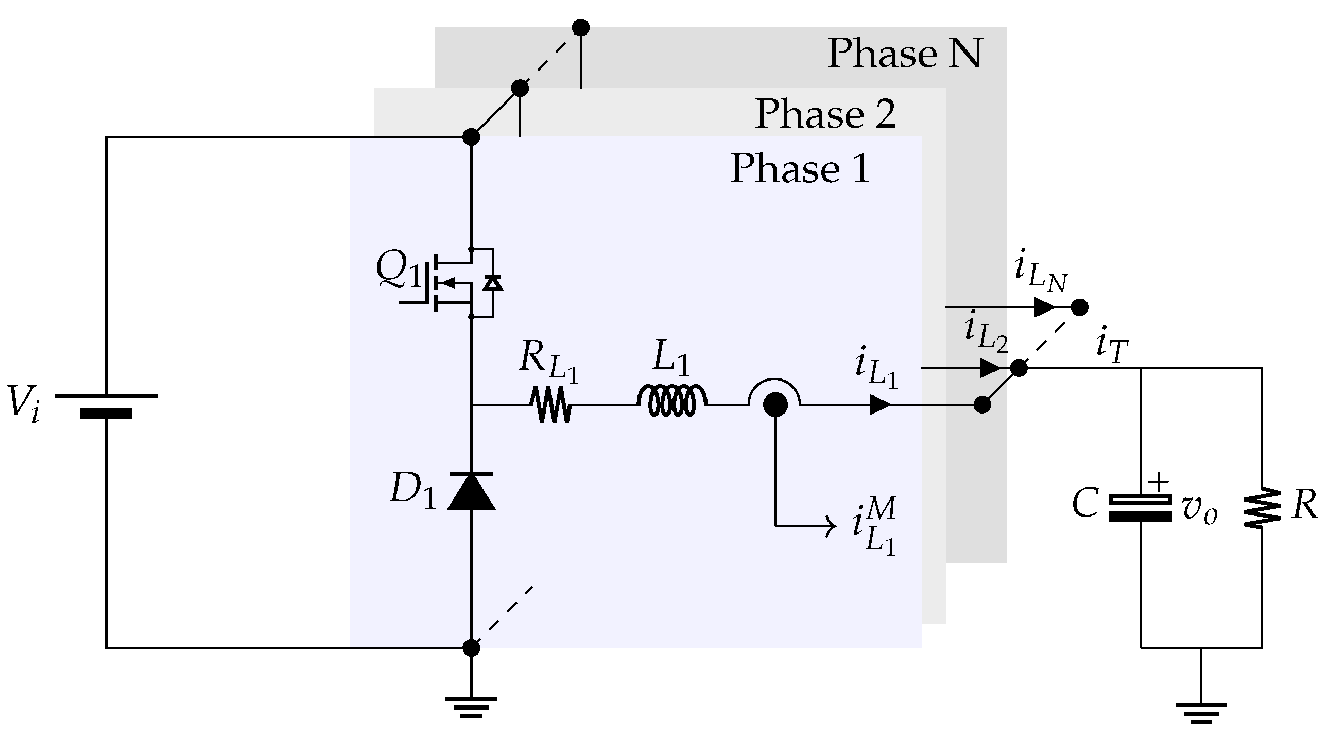
Figure 1 shows the schematic of a generalized interleaved buck converter for N branches or power stages. Each individual power stage is composed of a transistor $S_j$, a diode $D_j$, and an inductor $L_j$, considering the effect of its equivalent series resistance $R_j$, where the subscript $j=1,2,\dots ,N$ represents the branch number. All stages are connected to a common output capacitor C, and it is assumed that the converter powers a resistive load R. The reason for using this load is that the focus of this work is not on stabilizing the output voltage considering complex loads but rather on current equalization, distributing the load current equally among the branches, which in this case is given by $i_{L_j}=v_0/\left(NR\right)$.

Figure 1. Diagram of an N-phase interleaved buck converter.

2.1. Converter Model

The averaged model of the interleaved buck converter can be written as follows:

$$\begin{array}{ccc}\hfill {\displaystyle \frac{d{i}_{L_j}}{dt}}& =& {\displaystyle \frac{-R_{L_j}{i}_{L_j}}{L_j}}-{\displaystyle \frac{v_0}{L_j}}+{\displaystyle \frac{V_i}{L_j}}{\mu }_j,\hfill \\ \hfill {\displaystyle \frac{d{v}_0}{dt}}& =& \sum _{j=1}^N{\displaystyle \frac{i_{L_j}}{C}}-{\displaystyle \frac{v_0}{RC}},\hfill \end{array}$$

(1)

where $i_{L_j}$ are the inductor currents for each phase, $v_0$ is the output voltage, $V_i$ is the input voltage, and ${\mu }_j$ is the control signal for each switch.

2.2. Voltage Control and Current Balancing

This work employs a sliding mode (SM) control strategy based on Pulse Width Modulation (PWM) [32]. The control objectives of the interleaved buck converter are to regulate the output voltage to a desired value $V_{ref}$ and to balance the branch currents. To derive a control law that meets these objectives, the following sliding surfaces are proposed:

$${\sigma }_j={\displaystyle \frac{i_{ref}}{N}}-i_{L_j},$$

(2)

where $j=1,2,...,N$ corresponds to the number of branches or phases of the converter.

Furthermore, to ensure convergence to the surface in finite time, the following reaching law is proposed [33]:

$${\dot{\sigma }}_j=-\eta {\sigma }_j-\kappa \mathrm{sign}\left({\sigma }_j\right),$$

(3)

where $\eta$ and $\kappa$ are design constants.

The total current reference $i_{ref}$ is given by

$$i_{ref}=K_p(V_{ref}-v_o)+K_i\int (V_{ref}-v_o)dt,$$

(4)

where $K_p$ and $K_i$ are the gains of the proportional and integral correction terms, respectively.

By substituting Equation (4) into Equation (2) and differentiating it with respect to time—considering $V_{\mathrm{ref}}$ as the constant and utilizing the model information provided by Equation (1)—and equating it to Equation (3), it is possible to obtain the control actions for each branch ${\mu }_j$:

$${\mu }_j={\mu }_{eq,j}+{\mu }_{d,j},$$

(5)

where ${\mu }_{eq,j}$ is the equivalent sliding mode control and is given by

$${\mu }_{eq,j}={\displaystyle \frac{{\displaystyle \frac{K_p}{N}}\left({\displaystyle \frac{v_o}{CR}}-{\sum }_{j=1}^N{\displaystyle \frac{i_{L_j}}{C}}\right)+{\displaystyle \frac{K_i}{N}}(V_{ref}-v_o)+i_{L_j}{\displaystyle \frac{R_j}{L_j}}+{\displaystyle \frac{v_o}{L_j}}}{V_i/L_j}}.$$

(6)

The remaining term ${\mu }_{d,j}$ contains the discontinuous component of the control action and is given by

$${\mu }_{d,j}={\displaystyle \frac{\eta \sigma +\kappa \mathrm{sign}\left(\sigma \right)}{V_i/L_j}},$$

(7)

where the constants $\eta >0$ and $\kappa >0$ must be selected such that ${\mu }_{d,j}$ is a small fraction of the equivalent control, ensuring a convergence region based on the condition

$$0\le {\mu }_j\le 1.$$

(8)

In Figure 2, the trajectories of the sliding mode control adopted for the startup and different conditions are shown. According to (3), and if (8) is satisfied, it is ensured that the system will evolve to the surfaces ${\sigma }_j=0$ in finite time, and thus $i_{ref}/N=i_{L_j}$. It can be shown that $\eta >0$ and $\kappa >0$ are sufficient conditions for the global stability of the system, and that by selecting any $k_p>0$ and $k_i>0$, the system will always be stable regardless of the number of branches N.

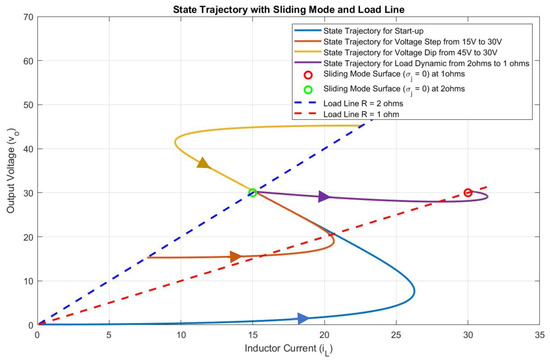
Figure 2. Trajectory of adopted sliding mode control.

3. Current Sensor Failures

A sensor failure represents abnormal operation and can generally be characterized as an open circuit failure, offset, or noise [34]. This section will analyze the impact of a current sensor failure on control and its estimation.

The current signal delivered by a faulty sensor, $i_{L_j}^M$, is represented as

$$i_{L_j}^M=i_{L_j}+{\gamma }_j,$$

(9)

where $i_{L_j}^M$ is the measured current, and ${\gamma }_j$ is the disturbance representing the failure of current sensor j, which generally corresponds to any of the aforementioned failure types.

For practical implementation, Equation (2) can be rewritten as

$${\sigma }_j={\displaystyle \frac{i_{ref}}{N}}-i_{L_j}^M.$$

(10)

In a first analysis, the converter control is assumed to be only current based, i.e., $i_{ref}=I_{ref}$, where $I_{ref}$ is a constant, and the current sensor in the phase k experiences a failure or disturbance ${\gamma }_k$. Therefore, in sliding mode, ${\dot{\sigma }}_k={\sigma }_k=0$, and in the event of a sensor failure, the current flowing through the inductor $L_k$ will be

$$i_{L_k}={\displaystyle \frac{I_{ref}}{N}}-{\gamma }_k.$$

(11)

On the other hand, the currents in the phases with healthy sensors are expressed as

$$i_{L_j}={\displaystyle \frac{I_{ref}}{N}},$$

(12)

with $k\ne j$.

This expression shows that, in the event of a current sensor failure, and with only current control being applied in the buck converter, only the current in the branch with the faulty sensor will be unbalanced. Therefore, in the case of a sensor fault, a simple failure detection strategy can be implemented. By using Equations (5) and (6), the following expression can be written:

$$i_{load}={\displaystyle \frac{v_o}{R}}\ne \sum _{j=1}^N{i}_{L_j}^M.$$

(13)

This brief analysis shows that the output current can be compared with the sum of the inductor currents, and any difference indicates an imbalance due to a sensor failure. This failure is easily identifiable in the case of a single sensor fault.

3.1. Influence of Sensor Failures on Current Balancing Considering the Effect of an External Voltage Loop

In the case where an external loop regulates the output voltage, the problem of current sensor fault detection becomes nontrivial. Although Equation (13) remains valid in the event of a sensor failure, identifying the faulty sensor becomes impossible, even in the case of a single faulty sensor. A detailed analysis of this issue is presented below.

Based on (10), the total reference current can be generally expressed as a function of the actual currents flowing through each inductor and the faults that the sensors may exhibit, represented as disturbances:

$$i_{ref}=\sum _{j=1}^N{i}_{L_j}^M=\sum _{j=1}^N(i_{L_j}+{\gamma }_j),$$

(14)

and additionally, using (4), the current reference under failure, $i_{ref}^{\gamma }$, is rewritten as

$$i_{ref}^{\gamma }=K_p(V_{ref}-v_o)+K_i\int (V_{ref}-v_o)dt+\sum _{j=1}^N{\gamma }_j,$$

(15)

from which it is clear that $i_{ref}^{\gamma }-i_{ref}={\sum }_{j=1}^N{\gamma }_j$.

Therefore, the branch current without sensor failure can be expressed as

$$i_{L_j}={\displaystyle \frac{i_{ref}}{N}}+\sum _{k=1}^N{\displaystyle \frac{{\gamma }_k}{N}},\mathrm{with}k\ne j,$$

(16)

and the actual current value in the phase with a sensor failure is written as

$$i_{L_j}={\displaystyle \frac{i_{ref}}{N}}-{\gamma }_j+\sum _{k=1}^N{\displaystyle \frac{{\gamma }_k}{N}}.$$

(17)

In the event of a failure, Equations (16) and (17) represent the deviation of the currents from the original current reference $i_{ref}$. This deviation is due to the disturbance ${\gamma }_j$ in conjunction with the integral action term included in the external voltage loop. This development shows that in a nested control scheme, a failure in one of the sensors will affect the rest of the currents, increasing the imbalance.

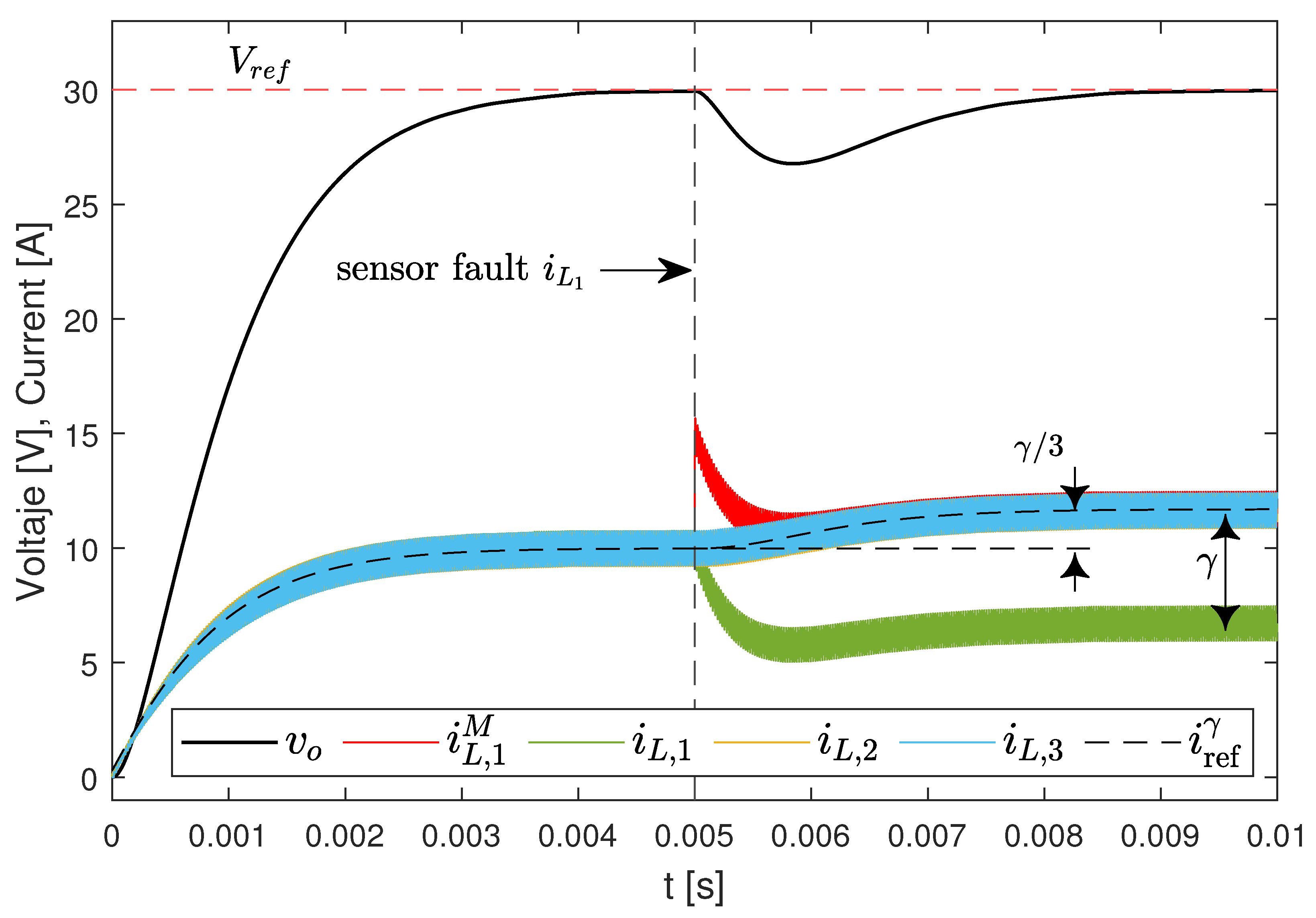
To further illustrate the above analysis, Figure 3 presents the simulation results for a three-phase converter ($N=3$), using the parameters listed in Table 1. At $t=0.005$ s, a fault is introduced in the current sensor of phase 1 with ${\gamma }_1=5$ [A], causing the measured current at that moment to be $i_{L,1}^M=15$ [A]. The balance control subsequently reduces $i_{L_1}^M$ and increases $i_{L_2}^M$ and $i_{L_3}^M$ until the measured currents reach equilibrium at $i_{ref}^{\gamma }=11.67$ [A] as described by Equation (16). Nevertheless, the actual current in phase 1 will be $i_{L_j}=6.67$ [A] according to Equation (17), exhibiting a clear imbalance due to the sensor fault.

Figure 3. Impact of sensor failure on current balancing control.

Table 1. Converter parameters.

Parameter	Description	Value
N	Branch Numbers	3
$V_i$	Input Voltage	60 V
R	Load Resistance	1 $\Omega$
C	Output Capacitor	0.22 mF
$L_j$	Inductor	60 μH
$R_j$	Resistance series with inductor	0.01 Ω
$f_s$	Switching Frequency	50 kHz
$K_p$	Proportional Gain	0.01
$K_i$	Integral Gain	9300
$\kappa$	Discontinuous gain term	700
$\eta$	Constant gain term	1500

3.2. Influence of Sensor Faults on Current Estimation

The use of observer-based methods for current estimation is beneficial in power converter applications, as they allow for the reduction in the number of required sensors and provide an attractive option for implementing fault-tolerant strategies. In particular, SMO demonstrates robustness against various types of disturbances, parametric variations, and unmodeled dynamics due to the incorporation of a discontinuous term for estimation correction [35]. However, this section presents an analysis of the performance of a SMO in estimating the phase currents of an interleaved buck converter in the presence of current sensor faults.

The model given by (1) can be written in a compact form as

$$\begin{array}{c}\dot{x}=Ax+B\mu ,\\ y=Cx+M_f\gamma ,\end{array}$$

(18)

where $x\in {\mathbb{R}}^n$ is the state vector, $A\in {\mathbb{R}}^{n\times n}$ is the system matrix, $B\in {\mathbb{R}}^{n\times m}$ is the input matrix, and $C\in {\mathbb{R}}^{n\times p}$ is the output matrix. $M_f$ is a fault distribution matrix $\in {\mathbb{R}}^{p\times q}$, where p is the number of measurable outputs, q is the number of unreliable or faulty sensors, and $\gamma \in {\mathbb{R}}^p$ is a vector representing the sensor faults, which is assumed to be bounded by $\left|\right|\gamma \left(t\right)\left|\right|<\alpha$.

Based on the converter model, it can be demonstrated that by selecting C to include $p=n-1$ measurable outputs, the system becomes observable. Thus, a sliding mode observer is proposed to estimate one of the currents using the measurements of the remaining currents and the output voltage. The goal is to demonstrate the estimation error that occurs in the presence of potential sensor faults.

The model given by (18) can be represented in canonical form using an orthogonal coordinate transformation $x\to T_{c}x$, where

$$T_c=\left[\begin{array}{c}{N}_c^T\\ C\end{array}\right],$$

(19)

is the transformation matrix whose submatrix $N_c$ spans the null space of C.

The system in the new coordinates is described by

$$\mathcal{A}=\left[\begin{array}{cc}{\mathcal{A}}_{11}& {\mathcal{A}}_{12}\\ {\mathcal{A}}_{21}& {\mathcal{A}}_{22}\end{array}\right],\mathcal{C}=\left[\begin{array}{cc}0& I_p\end{array}\right],$$

(20)

with ${\mathcal{A}}_{11}$∈${\mathbb{R}}^{(n-p)\times (n-p)}$, ${\mathcal{A}}_{21}$∈${\mathbb{R}}^{(n-p)\times p}$, ${\mathcal{A}}_{12}$∈${\mathbb{R}}^{p\times (n-p)}$ and ${\mathcal{A}}_{22}$∈${\mathbb{R}}^{(n-p)\times p}$ and $I_p$ is an identity matrix of order p.

In these new coordinates, an observer of the form can be proposed:

$$\begin{array}{c}\dot{\widehat{x}}=\mathcal{A}\widehat{x}+Bu-G_l{e}_y+G_n\nu \\ \widehat{y}=\mathcal{C}\widehat{x}\end{array},$$

(21)

where $\widehat{x}$ and $\widehat{y}$ are the estimates of x and y.

The discontinuous correction term $\nu$ is defined based on the output estimation error $e_{y,p}=\widehat{y_p}-y_p=C(\widehat{x}-x)$ as $\nu =\rho ,\mathrm{sign}\left(e_{y,p}\right)$, where $\rho$ is a positive constant. On the other hand,

$$G_n=\left[\begin{array}{c}L\\ -I_p\end{array}\right],$$

(22)

where $L=\left[L_1{L}_2{L}_3\right]$, and $G_l{e}_y$ is a linear correction term used to expand the convergence region to the sliding mode.

In the new coordinates and considering perturbed measurements, the error dynamics can be written as follows:

$$\begin{array}{ccc}\hfill {\dot{e}}_1& =& {\mathcal{A}}_{11}{e}_1+{\mathcal{A}}_{12}(e_y+M_f\gamma )+L\nu \hfill \\ \hfill {\dot{e}}_y+M_f\dot{\gamma }& =& {\mathcal{A}}_{21}{e}_1+{\mathcal{A}}_{22}(e_y+M_f\gamma )-\nu \hfill \end{array}.$$

(23)

To ensure the convergence of the errors $e_y$ to zero, $\rho$ must satisfy

$$\rho >\left|{\mathcal{A}}_{21}{e}_1+{\mathcal{A}}_{22}{e}_y\right|.$$

(24)

From the sliding mode conditions ($e_y=0$ and ${\dot{e}}_y=0$) and considering the steady state, that is, ${\dot{e}}_1=0$, the estimation error is obtained as

$$e_1={\displaystyle \frac{(-L{\mathcal{A}}_{22}{M}_f\gamma -{\mathcal{A}}_{12}{M}_f\gamma )+M_f\dot{\gamma }}{{\mathcal{A}}_{11}+L{\mathcal{A}}_{21}}}.$$

(25)

This equation demonstrates that, in the presence of a disturbance affecting the output of a measurable signal, an estimation error will arise. Specifically, with high gains and under the assumption that the disturbance varies slowly ($\dot{\gamma }\approx 0$), the estimation error will be approximately $e_1\approx \gamma$. This result is independent of the faulty sensor and holds true for any estimated current. To illustrate the case where high gains are employed, a simulation test is conducted using the observer described in Equation (21) on a 3-phase converter. The objective of the test is to estimate the phase 1 current, denoted as ${\widehat{i}}_{L,1}$, by measuring the remaining currents and the output voltage. Figure 4 presents the results of this test. During the interval $0.005\mathrm{s}\le t\le 0.015\mathrm{s}$, a fault in the current sensor $i_{L,1}$, characterized by ${\gamma }_1=5$ [A], is simulated. The measured current, $i_{L,1}^M$, is given by $i_{L,1}+{\gamma }_1$. It is observed that during this interval, the estimate $\widehat{i}L,1$ accurately tracks the mean value of the actual current in branch 1, $iL,1$. However, when a fault in the phase 2 sensor, denoted by ${\gamma }_2=5$ [A], occurs during the interval $0.025\mathrm{s}\le t\le 0.035\mathrm{s}$, the current estimate $\widehat{i}L,1$ becomes erroneous, following the mean value of the actual current $i_{L,2}$. This behavior can be generalized to any branch current, demonstrating the impossibility of accurately identifying the faulty sensor based solely on individual current measurements and estimates.

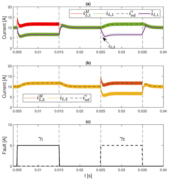
Figure 4. Effects of the fault in current estimation of ${\widehat{i}}_{L,1}$: (a) measured phase 1 current $i_{L,1}^M$, actual phase 1 current $i_{L,1}$, reference current $i_{\mathrm{ref}}$, and estimated current $\widehat{i}L,1$; (b) measured and actual phase 2 current, $i_{L,2}^M$ and $i_{L,2}$, respectively; (c) faults induced in the phase 1 and phase 2 sensors, ${\gamma }_1$ and ${\gamma }_2$, respectively.

4. Fault Reconstruction in Sensors

One way to identify sensor faults arises from Equation (25) in the previous development. If the matrix A is full rank, and considering that the disturbance is slowly varying ($\dot{\gamma }\approx 0$), the reconstruction of the sensor disturbance signal $\widehat{\gamma }$ in steady state (${\dot{e}}_1=0$) can be defined as

$$\widehat{\gamma }={(A_{21}{A}_{11}^{-1}{A}_{12}-A_{22})}^{-1}{\nu }_{eq}.$$

(26)

However, this estimation may present errors if the term $\dot{\gamma }$ is neglected. An effective solution to identify the faulty sensor is to use a dynamic fault reconstruction scheme through the use of filter banks [36]. Considering a new state vector $z_f$∈${\mathbb{R}}^p$, which consists of the filtered measurements of y,

$${\dot{z}}_f=-A_f{z}_f+A_{f}y,$$

(27)

where $A_f$∈${\mathbb{R}}^{p\times p}$ is a stable matrix.

Replacing y from (18),

$${\dot{z}}_f=-A_f{z}_f+A_{f}Cx+A_f{M}_f\gamma .$$

(28)

Based on Equations (18) and (28), the augmented state-space model of order $n+p$ is written as

$$\begin{array}{cc}\hfill {\dot{x}}_a& =A_a{x}_a+B_{a}u\left(t\right)+M_a\gamma ,\hfill \\ \hfill z_f& =C_a{x}_a,\hfill \end{array}$$

(29)

where $x_a={[x;z_f]}^T$ and the system matrices are given by

$$\begin{gathered} A_a=\left[\begin{array}{cc}A& 0\\ A_{f}C& -A_f\end{array}\right],B_a=\left[\begin{array}{c}B\\ 0\end{array}\right], \\ {M}_a=\left[\begin{array}{c}0\\ A_f{M}_f\end{array}\right],C_a=\left[0I_p\right]. \end{gathered}$$

(30)

One of the advantages of the augmented model given by (29) is that it allows expressing sensor faults as actuator faults. Thus, by designing an observer of order $n+p$, the fault vector $\gamma$ can be reconstructed using techniques applicable to these cases [16]. Figure 5 illustrates a simplified diagram of the fault reconstruction strategy, which is based on the design of an Edwards–Spurgeon observer. To facilitate this design, it is first necessary to perform a coordinate transformation of the form $x_a\to T_b{x}_a$:

$$\begin{array}{cc}\hfill {\dot{x}}_a& =A{x}_a+Bu\left(t\right)+M\gamma ,\hfill \\ \hfill y& =C{x}_a,\hfill \end{array}$$

(31)

with

$$\begin{gathered} \begin{array}{c}Aa=\left[\begin{array}{cc}{A}_{11}& A_{12}\\ \begin{array}{c}{A}_{211}\\ A_{212}\end{array}& A_{22}\end{array}\right],M=\left[\begin{array}{c}0\\ M_2\end{array}\right],\end{array} \\ C=\left[0T\right]. \end{gathered}$$

(32)

Here, $A_{11}\in {\mathbb{R}}^{(n+p)-p\times (n+p)-p}$, $A_{211}\in {\mathbb{R}}^{(p-q)-p\times (n+p)-p}$, $T\in {\mathbb{R}}^{p\times p}$ is an orthogonal matrix, and $M_2\in {\mathbb{R}}^{p\times q}$ has a structure in these coordinates:

$$M_2=\left[\begin{array}{c}0\\ M_o\end{array}\right],$$

(33)

where $M_o$ is nonsingular. It can be demonstrated that the transformation matrix $T_b$ will exist if $\mathrm{rank}\left(C_a{M}_a\right)=\mathrm{rank}\left(M_a\right)=q$, with $q<p$, and if the invariant zeros of $(A_a,M_a,C_a)$ are Hurwitz [16].

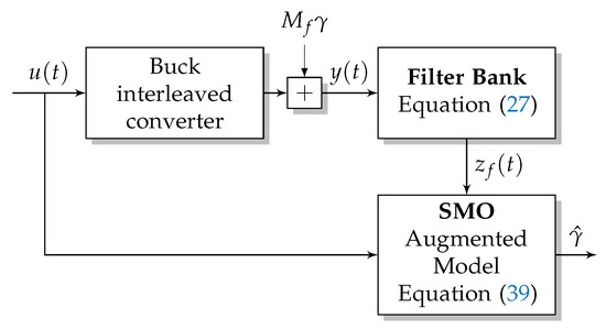
Figure 5. Scheme of the Fault Reconstruction Strategy.

In this work, it is assumed that all variables in the state vector are available as measurable and filtered outputs, i.e., $C_a=[0;I_n]$. Consequently, $T_b$ is constructed as follows:

$$T_b=\left[\begin{array}{cc}{I}_n& 0\\ 0& T^T\end{array}\right],$$

(34)

Additionally, T is constructed such that

$$T^T{A}_f{M}_f=\left[\begin{array}{c}0\\ M_o\end{array}\right].$$

(35)

Therefore, in the coordinates given by (32), and by designing an observer with the structure described by Equation (21) for the augmented model (29) of order $n+p$, the error dynamics are obtained as

$$\dot{e}=A_{o}e\left(t\right)+G_n\nu -M_f\gamma ,$$

(36)

where $A_o=(A-G_{l}C)$ and $e\left(t\right)={\widehat{x}}_a-x_a$. Regarding the design and gain matrices, $G_l$ is selected to ensure that $A_o$ is stable, and $G_n$ has the form:

$$G_n=\left[\begin{array}{c}-L\\ I_p\end{array}\right]T^T,L=\left[L_{o}0\right],$$

(37)

where the vector $L^o\in {\mathbb{R}}^{(n+p)-p\times (p-q)}$.

Finally, once the sliding mode is reached, with $e_y\left(t\right)={\dot{e}}_y\left(t\right)=0$, the error dynamics are given by

$$\begin{array}{cc}\hfill {\dot{e}}_1& =(A_{11}+L^0{A}_{211})e_1\left(t\right),\hfill \\ \hfill 0& =T{A}_{21}{e}_1\left(t\right)+{\nu }_{eq}-T{M}_2\gamma \left(t\right).\hfill \end{array}$$

(38)

With stable eigenvalues of $A_{11}+L^o{A}_{211}$, it is ensured that $e_1\to 0$, and from (38), the measurable reconstruction of the fault signal $\widehat{\gamma }\in {\mathbb{R}}^q$ can be defined as

$$\widehat{\gamma }={\left(M_2^T{M}_2\right)}^{-1}{M}_2^T{T}^T{\nu }_{eq},$$

(39)

where ${\left(M_2^T{M}_2\right)}^{-1}{M}_2^T{T}^T$ is the pseudo inverse matrix of $M_2$.

The advantage of this technique over the one proposed in Equation (26) is that it does not depend on $\dot{\gamma }$, and therefore provides a more accurate estimation of the fault signal.

However, the challenge of this technique lies in implementing the observer considering the augmented system. In other words, implementing the filter bank given by Equation (27) entails increasing the complexity and size of the circuit. It is possible to implement the strategy digitally both filter and SMO of the augmented model, as there are discrete design methods for sliding mode observers (SMOs) or numerical approximation methods that yield good results [37].

5. Results

The performance of the proposed method is evaluated through a numerical simulation analysis using the parameters listed in Table 1 and considering a converter with $N=3$ phases. To estimate the sensor faults using (39), an observer is designed with the structure of (21), in the coordinates given by (31), and considering $p=4$ measurable outputs ($i_{L_1}^M$, $i_{L_2}^M$, $i_{L_3}^M$, and $v_o$). Additionally, $A_f=3\times I_p$ is selected to filter the outputs, and the fault distribution vector is chosen as

$$M_f=\left[\begin{array}{c}{I}_q\\ 0\end{array}\right],$$

(40)

with $q=3$ corresponding to the number of current sensors, and $\gamma =[{\gamma }_1;{\gamma }_2;{\gamma }_3]$, it follows that all three current sensors are either deemed unreliable or prone to faults. Conversely, the gain matrix $G_l$ is designed to place the eigenvalues of $A_o$ at ${\lambda }_n=-9\times {10}^5$.

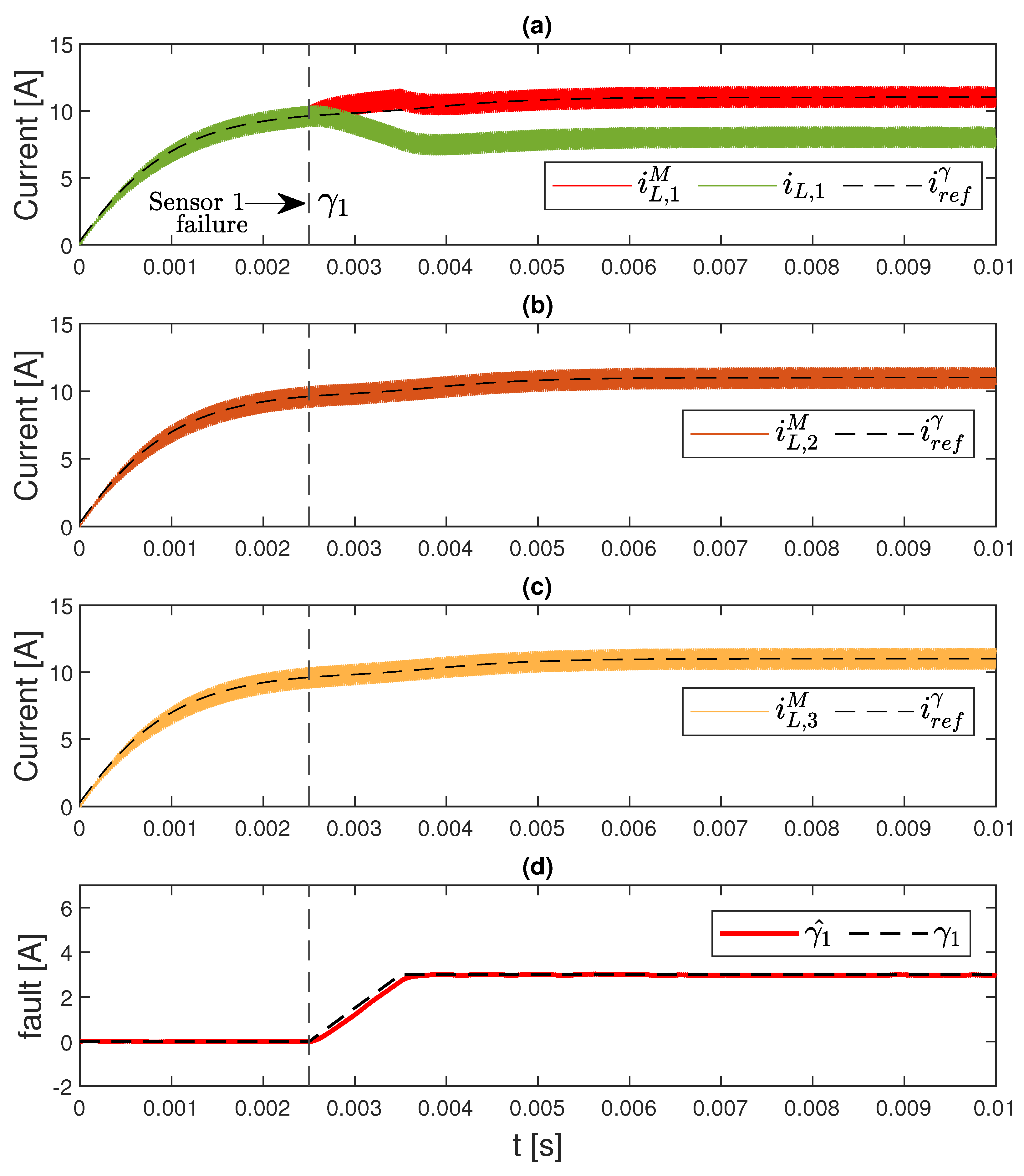
A first test is performed considering a fault in the phase 1 sensor, specifically $i_{L1}^M=i_{L_1}+{\gamma }_1$. The results of this test are shown in Figure 6. Figure 6a–c illustrate the evolution of the currents $i_{Lj}$ and their respective measurements $i_{Lj}^M$. Additionally, Figure 6d shows the emulated fault perturbation, ${\gamma }_1$, and its corresponding reconstruction, ${\widehat{\gamma }}_1$, using the technique proposed in this work. Initially, a voltage reference of $V_{ref}=30$ V is applied, and during the transient phase prior to the fault, all currents remain balanced. At time $t=0.0025$ s, a disturbance of ${\gamma }_1=3$ A is introduced, simulating an offset fault in the phase 1 sensor. As observed, due to the controller’s action, as detailed in Section 3, the currents converge to approximately $i_{\mathrm{ref}}^{\gamma }=11$ A. This leads to an imbalance, as the actual current in phase 1 becomes $i_{L1}=i_{L1}^M-{\gamma }_1=8$ A. Figure 6d demonstrates that, with this strategy, the disturbance is accurately estimated, unlike when using observers alone as discussed in Section 3.2.

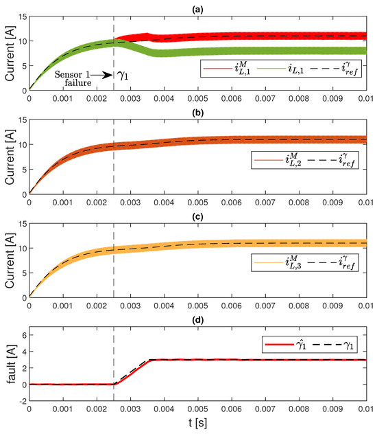
Figure 6. Fault reconstruction when a failure in sensor 1 occurs: (a) measured phase 1 current $i_{L,1}^M$, actual phase 1 current $i_{L,1}$, reference current $i_{\mathrm{ref}}$, and estimated current ${\widehat{i}}_{L,1}$; (b) measured and actual phase 2 current, $i_{L,2}^M$ and $i_{L,2}$, respectively; (c) measured and actual phase 3 current, $i^{M}L,3$ and $i_{L,3}$, respectively; (d) fault induced in the phase 1 ${\gamma }_1$ and its reconstruction ${\widehat{\gamma }}_1$.

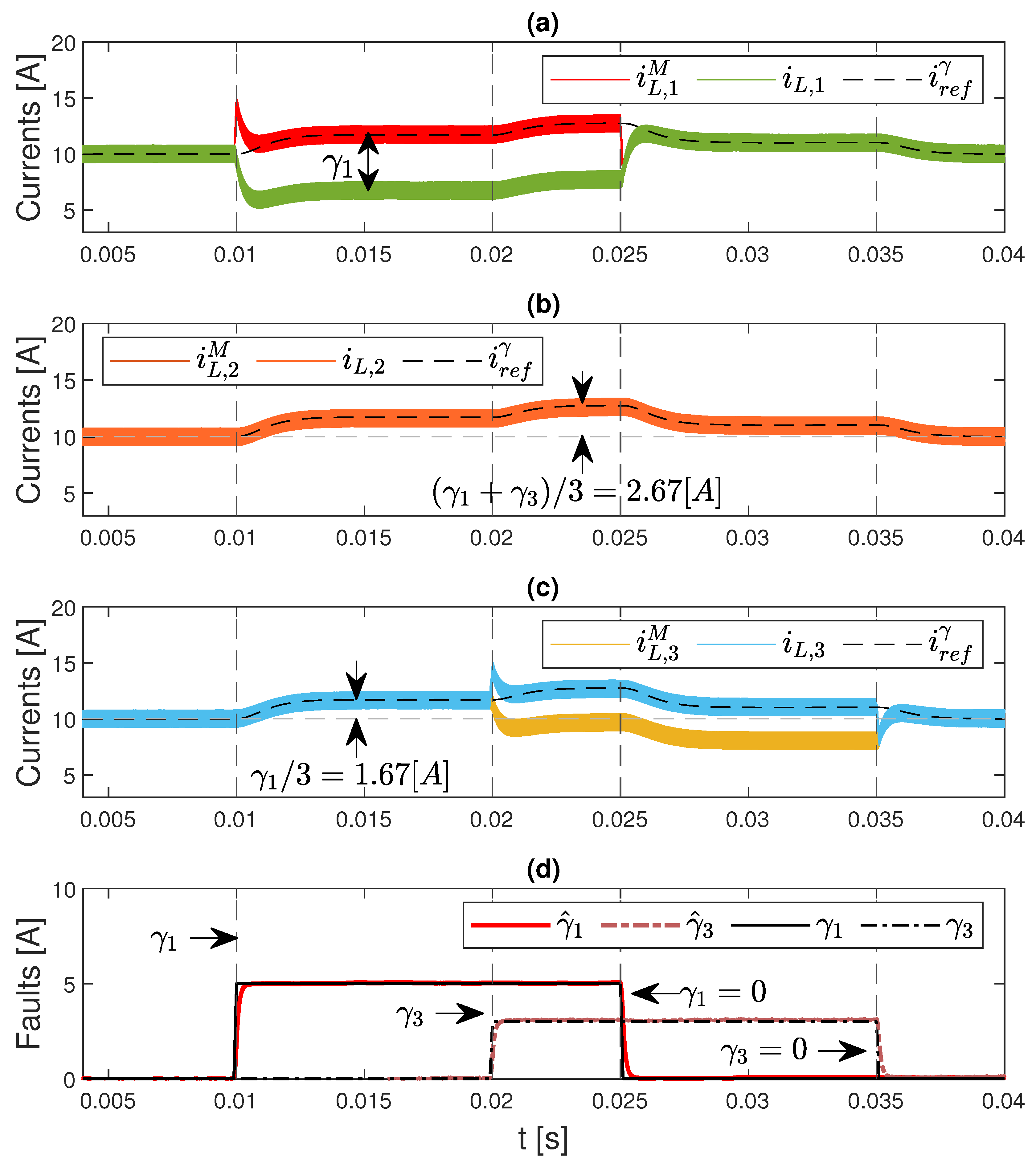
A second test is carried out to demonstrate the effectiveness of the strategy when simultaneous faults occur. Figure 7 shows the results of this test. First, a sensor fault in phase 1 is simulated during the interval $0.01\mathrm{s}\le t\le 0.025\mathrm{s}$. In Figure 7a, it can be observed that the actual current differs from the measured current due to fault ${\gamma }_1$, and it is correctly reconstructed by ${\widehat{\gamma }}_1$ (Figure 7d). During this time period, an imbalance in the phase currents occurs because the actual current of phase 1 will be $i_{L,1}=i_{L,1}^M-{\gamma }_1$. Additionally, it can be seen that this fault, due to the control action, affects the current reference, causing an increase in ${\gamma }_1/3=1.67$ [A]. Subsequently, during the interval $0.02\mathrm{s}\le t\le 0.035\mathrm{s}$, a fault of ${\gamma }_3=3\mathrm{A}$ is applied to sensor 3. It can be observed that the applied strategy correctly reconstructs both fault signals (${\widehat{\gamma }}_1$ and ${\widehat{\gamma }}_3$), even when they occur simultaneously. Moreover, it is also observed that when both sensors fail simultaneously, the new current reference is $i_{\mathrm{ref}}^{\gamma }=i_{\mathrm{ref}}+({\gamma }_1+{\gamma }_3)/3$ as shown in Equation (14).

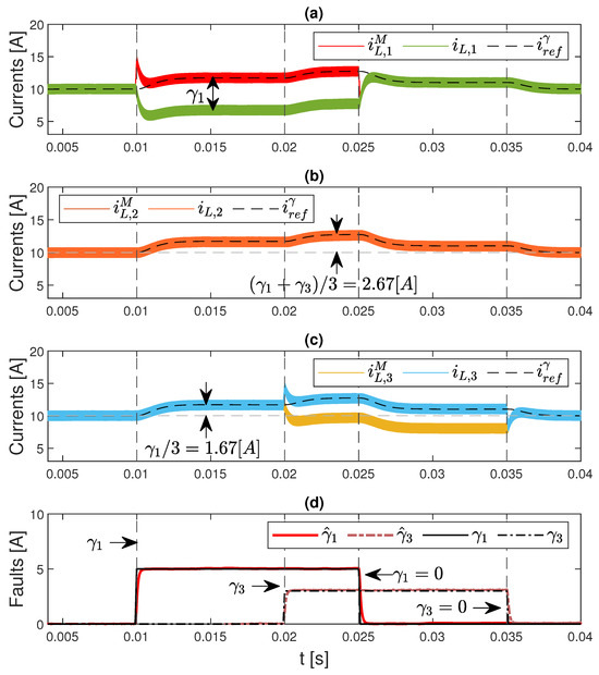
Figure 7. Fault reconstruction when a simultaneous failure occurs in sensors 1 and 2: (a) measured phase 1 current $i_{L,1}^M$, actual phase 1 current $i_{L,1}$, reference current $i_{\mathrm{ref}}$, and estimated current ${\widehat{i}}_{L,1}$; (b) measured and actual phase 2 currents, $i_{L,2}^M$ and $i_{L,2}$, respectively; (c) measured and actual phase 3 currents, $i^{M}L,3$ and $i_{L,3}$, respectively; (d) faults induced in phases 1 (black line) and 3 (black dashed line), ${\gamma }_1$ and ${\gamma }_3$ and their reconstruction ${\widehat{\gamma }}_1$ (red line) and ${\widehat{\gamma }}_3$ (red dashed line).

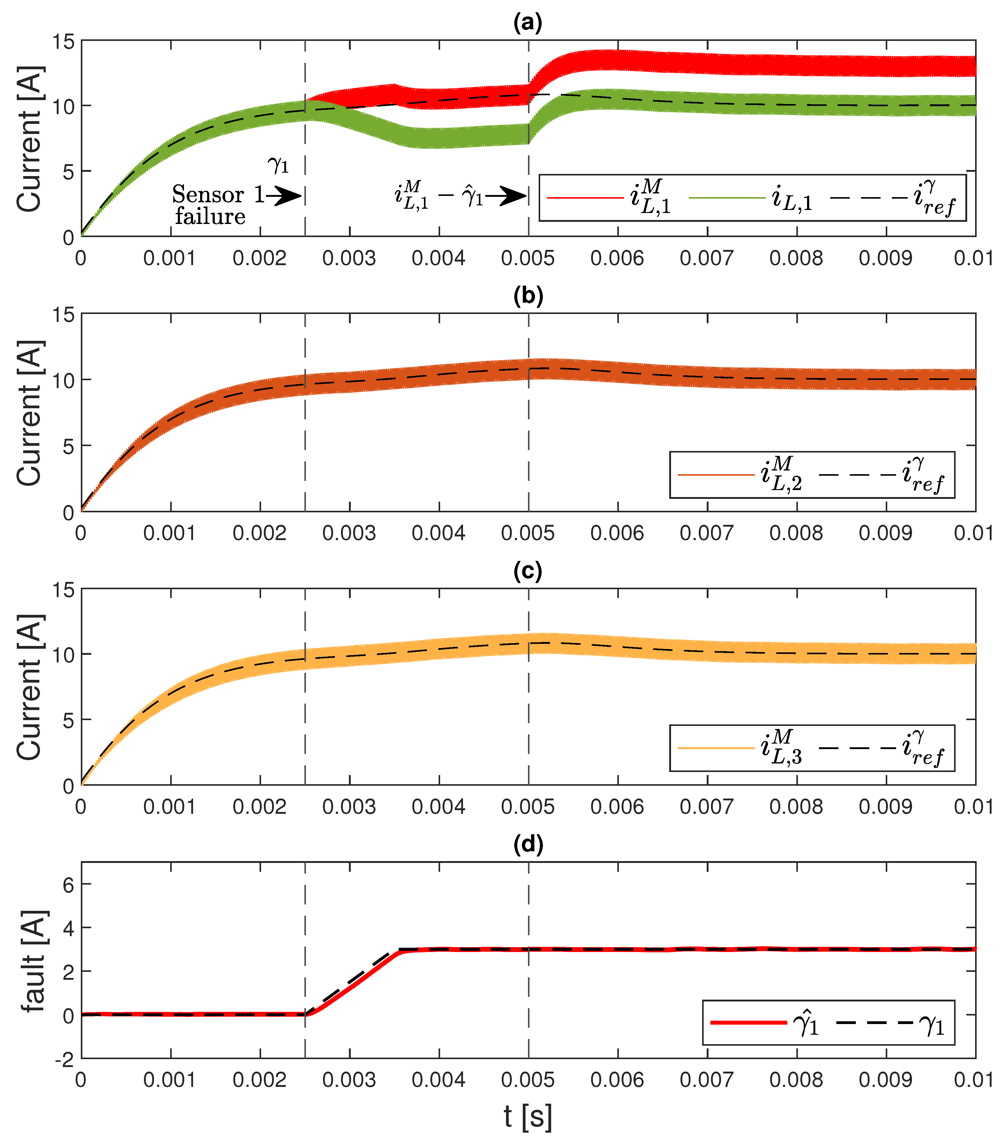
In order to demonstrate the capabilities of the strategy when implementing fault-tolerant strategies, in this case, a fault in phase 1 is simulated at $t=0.0025$ s, as in the first scenario. Once the fault is reconstructed at $t=0.005$ s, a fault-tolerant strategy is applied. Specifically, the surface of controller 1 is evaluated as ${\sigma }_1=i_{\mathrm{ref}}-i_{L,1}^M-{\widehat{\gamma }}_1$. The results for this test are shown in Figure 8. It can be observed that after correcting the faulty sensor signal, all currents are properly balanced, just as in the fault-free case.

Figure 8. Tolerant strategy when a failure in sensor 1 occurs: (a) measured phase 1 current $i_{L,1}^M$, actual phase 1 current $i_{L,1}$, reference current $i_{\mathrm{ref}}$, and estimated current ${\widehat{i}}_{L,1}$; (b) measured and actual phase 2 currents, $i_{L,2}^M$ and $i_{L,2}$, respectively; (c) measured and actual phase 3 currents, $i_{L,3}^M$ and $i_{L,3}$, respectively; (d) fault induced in the phase 1 ${\gamma }_1$ and its reconstruction ${\widehat{\gamma }}_1$.

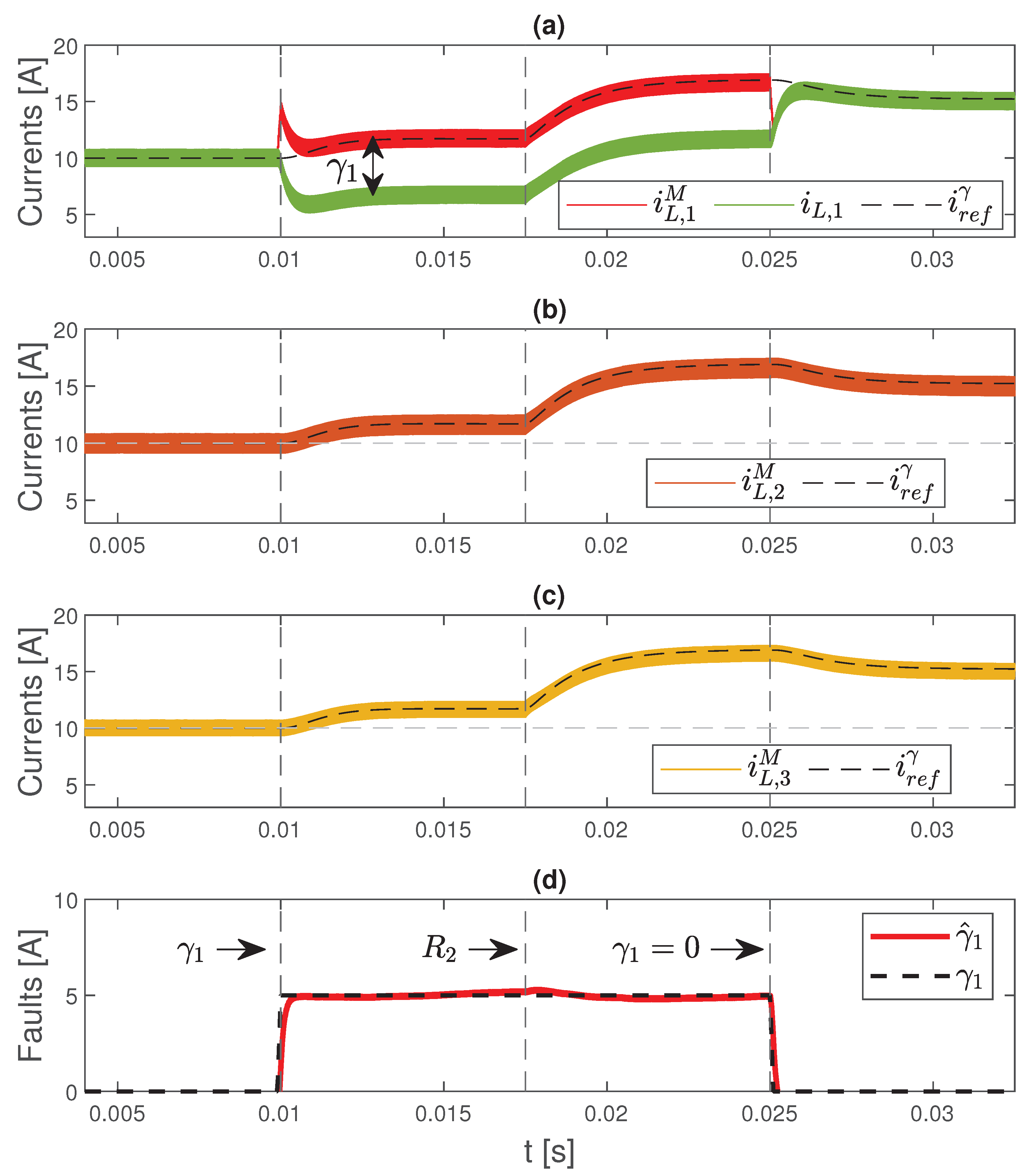
A final test is conducted to assess the performance of the strategy under parametric variations and load changes. A parametric variation in $L_2\to -10\%$, $L_3\to +10\%$, and $C\to 10\%$ is considered. Figure 9 shows the results of this test. It can be observed that when a fault, ${\gamma }_1$, occurs in the phase sensor at time $t=0.01$ s, the strategy successfully reconstructs the disturbance, ${\widehat{\gamma }}_1$, in the sensor without error. Additionally, at time $t=0.0175$ s, a load change is applied by introducing a new resistance $R_2=2R$ in parallel with the load resistance R. It is observed that in this case as well, the strategy continues to accurately reconstruct the disturbance.

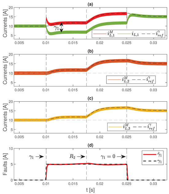
Figure 9. Results under parametric variations and load change: (a) measured phase 1 current $i_{L,1}^M$, actual phase 1 current $i_{L,1}$, reference current $i_{\mathrm{ref}}$, and estimated current $\widehat{i}L,1$; (b) measured and actual phase 2 currents, $i^{M}L,2$ and $i_{L,2}$, respectively; (c) measured and actual phase 3 currents, $i^{M}L,3$ and $i_{L,3}$, respectively; (d) fault induced in the phase 1 ${\gamma }_1$ and its reconstruction ${\widehat{\gamma }}_1$.

6. Conclusions

This paper presents a strategy for fault reconstruction in the current sensors of an interleaved buck DC–DC converter using a sliding mode observer. First, a detailed analysis and characterization of sensor faults and their adverse effects on current balancing and output voltage regulation controllers are performed. The impact of these faults on the design error of the current observer is then examined, highlighting the inability to identify which sensor is faulty by estimating the currents from the remaining phase currents and output voltage measurements. Regardless of the sensor or the estimated current, an estimation error is inevitable. Finally, a fault reconstruction strategy is proposed, using a filter bank to increase the system’s order and then designing an Edwards–Spurgeon observer. This approach treats the fault as if it were an actuator fault, enabling the application of a suitable reconstruction technique and subsequent identification of the faulty sensor. Using this strategy, correct fault reconstruction is achieved, treating the faults as disturbances in the current measurement, even when simultaneous faults occur. The proposed fault reconstruction can be implemented digitally; however, considerations and modifications will be necessary for discrete implementation. The setup of the experimental platform and the application of the proposed scheme will be initiated in future research.

References

- Alajmi, B.N.; Marei, M.I.; Abdelsalam, I.; Ahmed, N.A. Multiphase interleaved converter based on cascaded non-inverting buck-boost converter. IEEE Access 2022, 10, 42497–42506. [Google Scholar] [CrossRef]
- Cheng, X.F.; Peng, Z.; Yang, Y.; Liang, Z.; Wu, C.; Shao, Z.; Wang, D. A 5.6 kW 11.7 kW per kg Four-Phase Interleaved Buck Converter for the Unmanned Aerial Vehicle. J. Electr. Eng. Technol. 2022, 17, 1077–1086. [Google Scholar] [CrossRef]
- Koundi, M.; El Idrissi, Z.; El Fadil, H.; Belhaj, F.Z.; Lassioui, A.; Gaouzi, K.; Rachid, A.; Giri, F. State-Feedback Control of Interleaved Buck–Boost DC–DC Power Converter with Continuous Input Current for Fuel Cell Energy Sources: Theoretical Design and Experimental Validation. World Electr. Veh. J. 2022, 13, 124. [Google Scholar] [CrossRef]
- Ramos, R.; Biel, D.; Fossas, E.; Griñó, R. Sliding mode controlled multiphase buck converter with interleaving and current equalization. Control. Eng. Pract. 2013, 21, 737–746. [Google Scholar] [CrossRef]
- Aprilianto, R.A.; Ariefianto, R.M. Interleaving technique for improving conventional buck converter performance. In Proceedings of the 2022 International Conference on Technology and Policy in Energy and Electric Power (ICT-PEP), Bali, Indonesia, 3–5 September 2022; pp. 249–254. [Google Scholar]
- Ma, X.; Wang, P.; Wang, Y.; Tao, L.; Cheng, P. Penalty and Barrier-Based Numerical Optimization for Efficiency and Power Density of Interleaved Buck/Boost Converter. IEEE Trans. Power Electron. 2022, 37, 12095–12107. [Google Scholar] [CrossRef]
- Chen, H.C.; Lu, C.Y.; Rout, U.S. Decoupled master-slave current balancing control for three-phase interleaved boost converters. IEEE Trans. Power Electron. 2017, 33, 3683–3687. [Google Scholar] [CrossRef]
- Lu, L.; Li, Q.; Yang, Y.; Huang, Y.; Li, Z.; Zhang, D. Use of Threshold Median Adjustment to Achieve Accurate Current Balancing of Interleaved Buck Converter with Constant Frequency Hysteresis Control. Electronics 2024, 13, 3521. [Google Scholar] [CrossRef]
- Choi, H.-W.; Kim, S.-M.; Kim, J.; Cho, Y.; Lee, K.-B. Current-balancing strategy for multileg interleaved DC/DC converters of electric-vehicle chargers. J. Power Electron. 2021, 21, 94–102. [Google Scholar] [CrossRef]
- Viatkin, A.; Ricco, M.; Mandrioli, R.; Kerekes, T.; Teodorescu, R.; Grandi, G. Sensorless current balancing control for interleaved half-bridge submodules in modular multilevel converters. IEEE Trans. Ind. Electron. 2022, 70, 5–16. [Google Scholar] [CrossRef]
- Li, J.; Zhang, L.; Wu, X.; Zhou, Z.; Dai, Y.; Chen, Q. Current Estimation and Optimal Control in Multi-Phase DC–DC Converters with Single Current Sensor. IEEE Trans. Instrum. Meas. 2024, 73, 1–14. [Google Scholar]
- Mahmud, M.H.; Zhao, Y. Sliding mode duty cycle control with current balancing algorithm for an interleaved buck converter-based PV source simulator. IET Power Electron. 2018, 11, 2117–2124. [Google Scholar] [CrossRef]
- Yao, Z.; Lu, S. A Simple Approach to Enhance the Effectiveness of Passive Currents Balancing in an Interleaved Multiphase Bidirectional DC–DC Converter. IEEE Trans. Power Electron. 2019, 34, 7242–7255. [Google Scholar] [CrossRef]
- Xu, L.; Ma, R.; Xie, R.; Xu, J.; Huangfu, Y.; Gao, F. Open-circuit switch fault diagnosis and fault-tolerant control for output-series interleaved boost DC–DC converter. IEEE Trans. Transp. Electrif. 2021, 7, 2054–2066. [Google Scholar] [CrossRef]
- Kumar, G.K.; Elangovan, D. Review on fault-diagnosis and fault-tolerance for DC–DC converters. IET Power Electron. 2020, 13, 1–13. [Google Scholar] [CrossRef]
- Tan, C.P.; Edwards, C. Sliding mode observers for detection and reconstruction of sensor faults. Automatica 2002, 38, 1815–1821. [Google Scholar] [CrossRef]
- Zhuo, S.; Gaillard, A.; Xu, L.; Liu, C.; Paire, D.; Gao, F. An observer-based switch open-circuit fault diagnosis of DC–DC converter for fuel cell application. IEEE Trans. Ind. Appl. 2020, 56, 3159–3167. [Google Scholar] [CrossRef]
- Ribeiro, E.; Cardoso, A.J.M.; Boccaletti, C. Open-circuit fault diagnosis in interleaved DC–DC converters. IEEE Trans. Power Electron. 2013, 29, 3091–3102. [Google Scholar] [CrossRef]
- Li, C.; Yu, Y.; Yang, Z.; Wang, W.; Peng, X. A Sensorless Open-Circuit Fault Identification Method for Interleaved Boost Converter. IEEE Trans. Instrum. Meas. 2024, 73, 1–8. [Google Scholar] [CrossRef]
- Ahmad, M.W.; Gorla, N.B.Y.; Malik, H.; Panda, S.K. A fault diagnosis and postfault reconfiguration scheme for interleaved boost converter in PV-based system. IEEE Trans. Power Electron. 2020, 36, 3769–3780. [Google Scholar] [CrossRef]
- Zhuoxun, L.; Zhengwang, X.; Xiaohua, Z. A novel real-time fast fault-tolerance diagnosis and fault adjustment strategy for m-phase interleaved boost converter. IEEE Access 2021, 9, 11776–11786. [Google Scholar]
- Mahdavi, M.S.; Karimzadeh, M.S.; Rahimi, T.; Gharehpetian, G.B. A fault-tolerant bidirectional converter for battery energy storage systems in DC microgrids. Electronics 2023, 12, 679. [Google Scholar] [CrossRef]
- Aviña-Corral, V.; Rangel-Magdaleno, J.d.J.; Barron-Zambrano, J.H.; Rosales-Nuñez, S. Review of fault detection techniques in power converters: Fault analysis and diagnostic methodologies. Measurement 2024, 234, 114864. [Google Scholar] [CrossRef]
- Li, J.; Pan, K.; Zhang, D.; Su, Q. Robust fault detection and estimation observer design for switched systems. Nonlin. Anal. Hybrid Syst. 2019, 34, 30–42. [Google Scholar] [CrossRef]
- Narzary, D.; Veluvolu, K.C. Higher order sliding mode observer-based sensor fault detection in DC microgrid’s buck converter. Energies 2021, 14, 1586. [Google Scholar] [CrossRef]
- Li, J.; Zhang, Z.; Li, B. Sensor fault detection and system reconfiguration for DC–DC boost converter. Sensors 2018, 18, 1375. [Google Scholar] [CrossRef]
- Schmidt, S.; Oberrath, J.; Mercorelli, P. A sensor fault detection scheme as a functional safety feature for DC–DC converters. Sensors 2021, 21, 6516. [Google Scholar] [CrossRef]
- Silveira, A.M.; Araújo, R.E. A new approach for the diagnosis of different types of faults in dc–dc power converters based on inversion method. Electr. Power Syst. Res. 2020, 180, 106103. [Google Scholar] [CrossRef]
- Li, J.; Pan, K.; Su, Q.; Zhao, X.-Q. Sensor fault detection and fault-tolerant control for buck converter via affine switched systems. IEEE Access 2019, 7, 47124–47134. [Google Scholar] [CrossRef]
- Poon, J.; Jain, P.; Konstantakopoulos, I.C.; Spanos, C.; Panda, S.K.; Sanders, S.R. Model-based fault detection and identification for switching power converters. IEEE Trans. Power Electron. 2016, 32, 1419–1430. [Google Scholar] [CrossRef]
- Al-Sheikh, H.; Hoblos, G.; Moubayed, N.; Karami, N. A sensor fault diagnosis scheme for a DC/DC converter used in hybrid electric vehicles. IFAC-PapersOnLine 2015, 48, 713–719. [Google Scholar] [CrossRef]
- Wang, J.; Li, S.; Yang, J.; Wu, B.; Li, Q. Extended state observer-based sliding mode control for PWM-based DC–DC buck power converter systems with mismatched disturbances. IET Control. Theory Appl. 2015, 9, 579–586. [Google Scholar] [CrossRef]
- Wu, L.; Liu, J.; Vazquez, S.; Mazumder, S.K. Sliding mode control in power converters and drives: A review. IEEE/CAA J. Autom. Sin. 2021, 9, 392–406. [Google Scholar] [CrossRef]
- Li, J.; Pan, K.; Su, Q. Sensor fault detection and estimation for switched power electronics systems based on sliding mode observer. Appl. Math. Comput. 2019, 353, 282–294. [Google Scholar] [CrossRef]
- Shahzad, E.; Khan, A.U.; Iqbal, M.; Saeed, A.; Hafeez, G.; Waseem, A.; Albogamy, F.R.; Ullah, Z. Sensor fault-tolerant control of microgrid using robust sliding-mode observer. Sensors 2022, 22, 2524. [Google Scholar] [CrossRef]
- Alwi, H.; Edwards, C.; Tan, C.P. Fault Detection and Fault-Tolerant Control Using Sliding Modes; Springer: Berlin/Heidelberg, Germany, 2011. [Google Scholar]
- Da Silva, G.S.; Vieira, R.P.; Rech, C. Discrete-time sliding-mode observer for capacitor voltage control in modular multilevel converters. IEEE Trans. Ind. Electron. 2017, 65, 876–886. [Google Scholar] [CrossRef]
Disclaimer/Publisher’s Note: The statements, opinions and data contained in all publications are solely those of the individual author(s) and contributor(s) and not of MDPI and/or the editor(s). MDPI and/or the editor(s) disclaim responsibility for any injury to people or property resulting from any ideas, methods, instructions or products referred to in the content. |
© 2024 by the authors. Licensee MDPI, Basel, Switzerland. This article is an open access article distributed under the terms and conditions of the Creative Commons Attribution (CC BY) license (https://creativecommons.org/licenses/by/4.0/).