Abstract
Electronic speckle pattern interferometry (ESPI) is widely used in fields such as materials science, biomedical research, surface morphology analysis, and optical component inspection because of its high measurement accuracy, broad frequency range, and ease of measurement. Phase extraction is a critical stage in ESPI. However, conventional phase extraction methods exhibit problems such as low accuracy, slow processing speed, and poor generalization. With the continuous development of deep learning in image processing, the application of deep learning in phase extraction from electronic speckle interferometry images has become a critical topic of research. This paper reviews the principles and characteristics of ESPI and comprehensively analyzes the phase extraction processes for fringe patterns and wrapped phase maps. The application, advantages, and limitations of deep learning techniques in filtering, fringe skeleton line extraction, and phase unwrapping algorithms are discussed based on the representation of measurement results. Finally, this paper provides a perspective on future trends, such as the construction of physical models for electronic speckle interferometry, improvement and optimization of deep learning models, and quantitative evaluation of phase extraction quality, in this field.
1. Introduction
Electronic speckle pattern interferometry (ESPI) is a nondestructive optical measurement technique known for its simplicity, high speed, large field of view, excellent anti-interference performance, and suitability for dynamic measurements [1,2,3,4]. ESPI has numerous research applications in fields such as industry and engineering, including strain [5,6], displacement [7,8], vibration measurements [9,10], and material defect detection [11,12]. Phase information can be extracted by analyzing the interference fringe image, and the measured physical quantities, such as displacement and deformation, are closely related to the phase. As a result, one challenge in ESPI is the accurate extraction of phase information from interference fringe images for the analysis of the measured physical phenomena. Therefore, the difficulty, accuracy, generalization, and extraction speed of phase extraction methods are crucial for this technology.
Typically, image sensors and human eyes perceive and record the intensity distribution of light field through the photoelectric conversion effect. Because the frequency of a light wave being much larger than the sampling frequency, it is impossible to directly perceive and record the phase information of a light field. Fortunately, the phase delay changes the intensity distribution as the light field propagates. Consequently, the corresponding phase distribution can be deduced from the recorded light field intensity distribution, and the physical quantity to be measured can then be calculated through the phase transformation [13]. This process is known as phase extraction.
Current methods for phase extraction in ESPI can be categorized into two types, namely classical phase extraction methods, which are represented by techniques such as phase shifting [14] and carrier methods [15], and emerging data-driven methods based on deep learning. Phase shifting methods consider the known phase differences between multiple frames of fringe patterns, whereas carrier methods consider the frequency spectrum distribution characteristics of fringe patterns to extract phase information. Classical phase extraction methods have been widely used in industrial engineering, providing rich phase information and enabling economical and efficient noncontact full-field measurements. However, these methods involve complex and cumbersome steps requiring manual parameter tuning. Furthermore, dealing with noise, background interference, and phase discontinuities remains challenging. These challenges necessitate researchers to investigate novel methods for addressing these problems.
Deep learning network models, with convolutional neural networks (CNN) as a representative, have demonstrated the capability to extract complex features and patterns from images and achieved satisfying results in computer vision, data image processing, and related fields [16]. Some scholars have introduced deep learning into ESPI phase extraction and achieved notable results [17].
Because of the differences in measurement methods, the measurement results of ESPI technology typically manifest as ESPI fringe patterns or ESPI-wrapped phase maps. Deep learning methods are increasingly being used in both these results. This paper provides an overview of the fundamental principles and image characteristics of ESPI, emphasizing the application of existing deep learning methods in these two distinct measurement results. In addition, this paper compares the performance of various deep learning methods and highlights their advantages in addressing the challenges faced by conventional methods. Furthermore, the limitations of existing methods are detailed, and a prospective analysis of the development trends, covering aspects such as the construction of physical models for ESPI, improvement and optimization of deep learning models, and quantitative evaluation of phase extraction quality, is presented. This paper provided valuable insights for the advancement of phase extraction in ESPI.
The main contributions of this paper are as follows:
- (1)
- The application of the existing deep learning methods for phase extraction in the field of ESPI is comprehensively analyzed and summarized. By comparing the performance of different methods and the potential advantages of deep learning compared with traditional methods, this paper provides readers with a comprehensive understanding and evaluation of this topic.
- (2)
- The development prospects of deep learning methods for phase extraction in the field of ESPI are explored. This paper discusses the possible challenges of current deep learning methods in ESPI phase extraction, and it proposes directions for future improvement and development to provide a reference for researchers.
- (3)
- This paper provides knowledge and guidance for scholars who want to use deep learning methods to measure ESPI strain and displacement in the future.
2. Production of ESPI Images
Speckle was initially regarded as a common optical phenomenon. However, in holography, speckles considerably affect the quality of holographic images Therefore, in holography, speckles are considered noise, and reduction of speckle interference is a critical topic of research. In 1966, Ennos [18] discovered that randomly distributed speckles can be used as information carriers, including information on light intensity and phase. Since then, people have conducted considerable research on speckle measurement technology. In ESPI, a charge-coupled device is used to record speckle images, which are processed on a computer. Speckle is a noncontact full-field optical measurement method. This technology overcomes the limitations of previous optical measurement technology applications and is a speckle interferometric measurement method implemented by electronics and digital methods. This method has high accuracy, rapid response, and full-field noncontact.
Currently, the ESPI technology measurement system consists of several key components, including lasers, CCD cameras, computers, image acquisition cards, and some optical elements. Figure 1 displays a typical ESPI measurement optical path, where M represents a reflective prism, and BS1 and BS2 are spectral prisms. The laser beam is categorized into a measurement beam and a reference beam after passing through spectral prism BS1, and the measurement beam is irradiated onto the measured object. After passing through the beam expander, the measurement beam interferes with the reference beam after passing through reflective prism BS2, and the CCD camera records interference fringes, transfers the image information to the computer for processing, and displays the test results in real time.
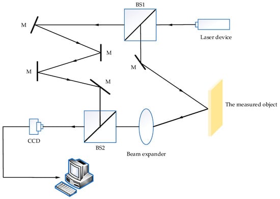
Figure 1.
A typical ESPI measurement optical path.
The recorded speckle information before and after object deformation is expressed as follows:
where and represent the intensity of the speckle field before and after deformation, respectively; and represent the intensity of the two coherent beams, respectively; is the phase difference in the speckle field on the object plane; is the change inphase difference caused by object deformation. The relationship between and deformation displacement is as follows:
By subtracting the light intensity of the speckle pattern before and after the deformation of the measured object, as follows:
With the change in the value of , the light intensity difference also changes, which allows us to observe fringe information that is not visible in a certain light field intensity, resulting in alternating bright and dark fringe images.
The measurement results of ESPI are usually the ESPI fringe pattern derived from the formula and the ESPI-wrapped phase map obtained by installing a phase shifter on the reference optical path and using a stepwise phase shift. As displayed in Figure 2, both contain considerable noise, and the ESPI fringe pattern presents a black and white, alternating light and dark fringe structure, with the density and direction of the fringes reflecting the phase difference changes on the object surface. The ESPI-wrapped phase map limits the phase information to the range and displays it in grayscale or pseudo-color. The physical quantity to be measured is directly related to the phase distribution information of both. Therefore, studying advanced electronic speckle interferometry phase extraction methods is critical for quickly and accurately analyzing the measured physical quantity from the ESPI fringe pattern or wrapped phase map and has become a critical topic of research in current ESPI.
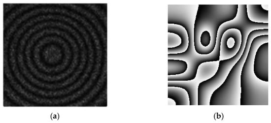
Figure 2.
Two measurement results of ESPI technology ((a) ESPI fringe pattern and (b) ESPI-wrapped phase map).
3. Application of Deep Learning in the Phase Extraction of ESPI Fringe Patterns
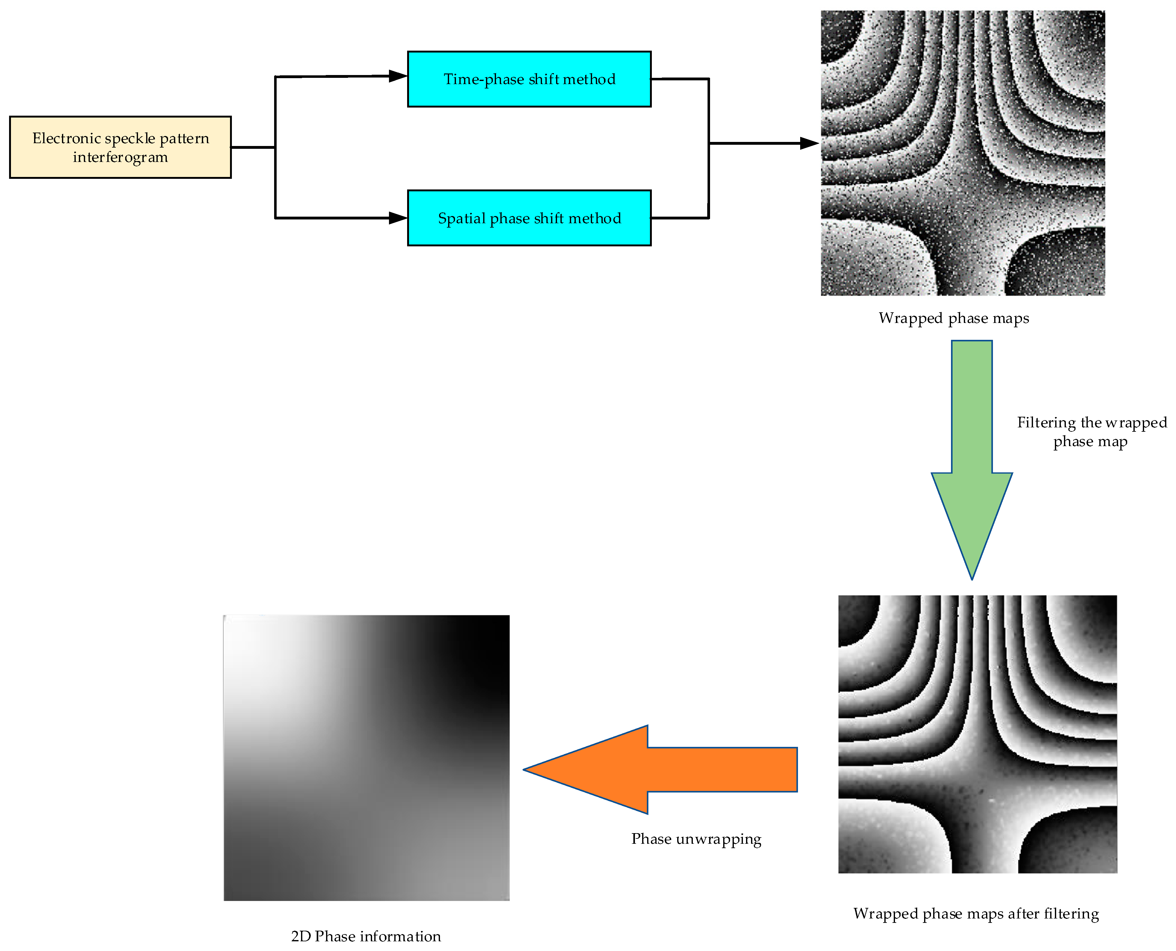
The fringe centerline method is a classic phase extraction method for ESPI fringe patterns. Compared with other phase extraction methods, such as Fourier transform and wavelet transform, the fringe centerline method is the most direct phase extraction method based on a single fringe pattern. In this method, first, the fringe pattern is filtered for noise removal, the skeleton line of the ESPI fringe pattern is extracted, the series of skeleton lines is identified, and the phase values at the location of the skeleton lines are obtained. Finally, a specific algorithm was used to interpolate the identified skeleton lines to obtain full-field phase information. Figure 3 displays the steps of the method. The following sections explain the application of deep learning in this method.
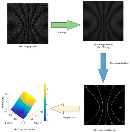
Figure 3.
Phase extraction steps of ESPI fringe pattern [19].
3.1. Application of Deep Learning in ESPI Fringe Pattern Filtering
The ESPI fringe pattern obtained from actual measurement contains considerable speckle noise. Therefore, prior to extracting the phase, the first step is to perform filtering processing. According to the various densities of fringes, the ESPI fringe pattern can be categorized into low-density fringe pattern, high-density fringe pattern, variable-density fringe pattern, and discontinuous fringe pattern. Conventional fringe pattern filtering methods include the sine and cosine mean method, the window Fourier transform method, and the two-dimensional wavelet transform method [20]. These methods are classified according to various objects. In the actual processing process, the following problems are persistent:
- (1)
- Slow processing speed, rendering handling multiple frames simultaneously impossible.
- (2)
- Suboptimal denoising effect on complex images, such as high- and variable-density ESPI fringe patterns.
- (3)
- Poor generalization, necessitating repeated fine-tuning for various objects, and lack of a general model.
- (4)
- Substantial computational parameters.
To address the problems of slow speed and the inability to process multiple frames simultaneously in conventional filtering methods, in 2019, Hao et al. from Tianjin University were inspired by the FFD-Net model [21] and introduced it into ESPI fringe pattern denoising [22]. This method can process 50 images simultaneously and requires only 8 s for processing, but the speed of the method is slow.
In 2020, Lin et al. [23] from Shandong University addressed the challenge of poor denoising performance of conventional methods for ESPI fringe patterns with high variation in density. They introduced the FPD–CNN network, which considerably outperformed the conventional windowed Fourier transform (WFT) method and coherence enhancing diffusion (CED) method, achieving the peak-signal-to-noise ratio (PSNR), the mean of structural similarity index (SSIM), and the mean absolute error (MAS) metrics of 27.88 (dB), 0.972, and 7.642, respectively, at a processing speed of just 0.57 s (Figure 4). The FPD–CNN method provides superior denoising performance for fringe patterns with varying densities. In 2022, Wang et al. [24] from Shenyang Aerospace University incorporated the squeeze and excitation (SE) attention mechanism into the DnCNN denoising model, introducing the AD-CNN network for ESPI fringe pattern denoising. This method achieved a PSNR of 20.1532 (dB) on a self-made dataset, surpassing the performance of the classic denoising model DnCNN and the WFF method, which achieved PSNR values of 17.0934 and 17.0068 dB, respectively.
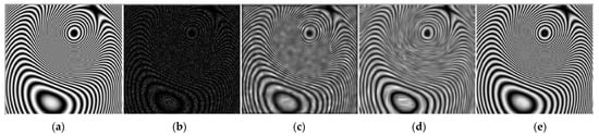
Figure 4.
Comparison of denoising high-variation density fringe patterns obtained using various methods [23]. (a) Noise-free image. (b) Noisy image. (c) WFF method. (d) CED method. (e) FPD-CNN method.
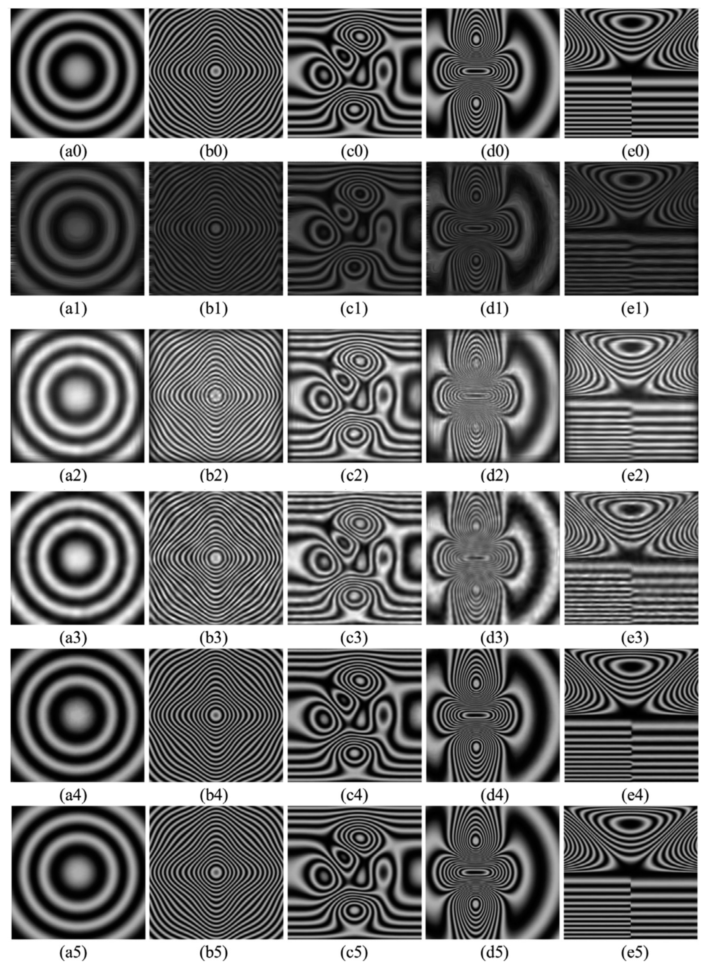
To improve the generalization ability of the model, in 2022, Xu et al. from Tianjin University [25] constructed an MDD-Net network model using a skip connection method to filter various types of ESPI fringe patterns. The team applied this method to the measurement of the out-of-plane displacement of thermal changes in PCB boards, and its measurement accuracy can reach the nanometer level. This method outperforms existing SOOPDE, WFF, and BL-Hilbert-L2 methods in terms of detail protection, speckle reduction, and shape preservation under various types of density fringes. MDD-Net outperforms the FFD-Net proposed in reference [22] in discontinuous density fringe filtering denoising, the former having an SNR of 40.6 and SSIM of 0.991, which are superior to the latter’s SNR of 38.387 and SSIM of 0.965, indicating its superior generalization ability. Figure 5 displays the specific filtering effect.
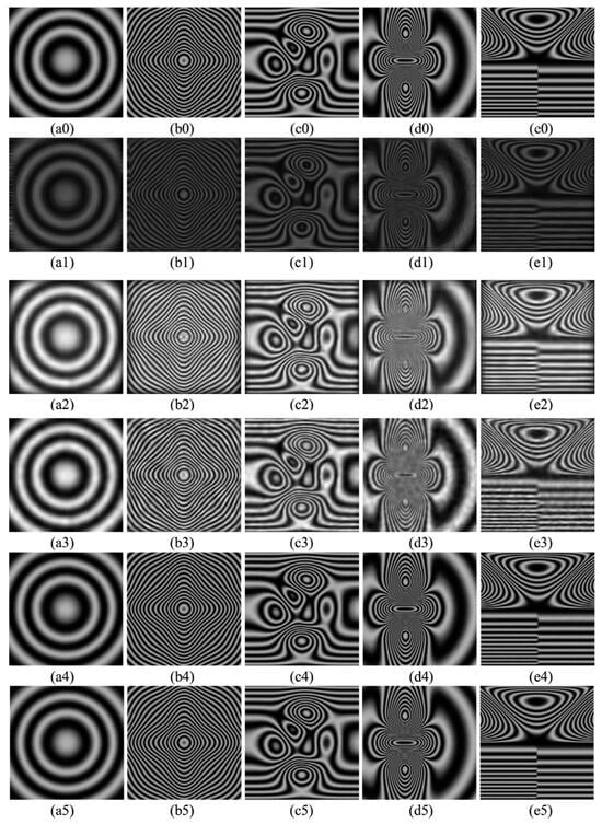
Figure 5.
Comparison experiments of ESPI fringe pattern filtering (a–e), respectively represent low-density, high-density, variable-density, greatly variable density, and discontinuous fringe samples. (a0–e0), (a1–e1), (a2–e2), (a3–e3), (a4–e4), and (a5–e5) are the true labels of the simulated ESPI fringe patterns, SOOPDE, WFF, BL-Hilbert-L2, FDD-Net, and MDD-Net methods, respectively) [25].
This research achieved considerable success in terms of generalization and accuracy, but increased the model parameter size and reduced the processing speed. To solve this problem, in 2022, Gurrola-Ramos et al. from the Mathematics Research Center, Guanajuato, Mexico, proposed a lightweight residual dense network based on the U-Net structure (LRDUNet) [26]. This network reduced the number of parameters using grouped convolution and density convolution modules. The number of parameters in this method was only 4.21 M, and the processing speed reached 0.00665 s. This method has excellent denoising performance, with a PSNR of 40.1427 dB. Figure 6 displays the specific structure of this network.
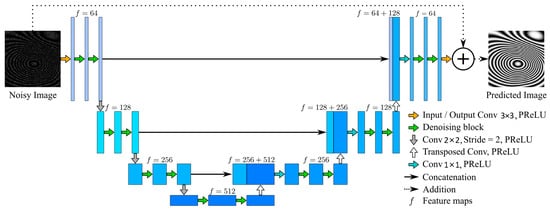
Figure 6.
LRDUNet network model [26].
Table 1 compares the denoising performance indicators for each model, where the “Parameters” values of the FFD-Net and MDD-Net model were converted from the literature [22,26], respectively. The conversion formula is 1 M = 1024 K.

Table 1.
Comparison of denoising performance indicators for each model [21,23,24,25,26].
In the above formula, is the number of samples in the dataset, and and prime represent the true value and predicted value of the ith sample, respectively. is the maximum value of the image point color; if each sample point is represented by 8 bits, then it is 255. μx and μy represent the mean values of images and , respectively. and represent the variances of images and , respectively. represents the covariance of images and . and are constants.
The existing deep learning ESPI fringe pattern denoising methods require large models with poor generalization to different types of fringe patterns. Therefore, future development requires adaptability, high accuracy, and small model parameters.
3.2. Application of Deep Learning in the Fringe Skeleton Extraction Method
After filtering, the fringe skeleton lines should be extracted. The quality of skeleton line extraction directly affects the accuracy of phase extraction. The conventional fringe skeleton line is based on image binarization technology, which performs morphological operations and connectivity analysis on binarized images to extract fringe skeleton lines. Early representative skeleton extraction methods included a binarization threshold refinement algorithm [27], stripe peak tracking method [28], and binary graph method based on two-dimensional derivative symbols [19]. Subsequent studies have considered the characteristics of stripe direction and proposed new stripe skeleton line extraction methods, such as the coupled gradient vector flow field method [29], direction-coupled gradient vector flow field extraction method [30], anisotropic gradient vector flow field extraction method [31], and gradient vector field of variational image segmentation solution [32]. The conventional fringe skeleton line extraction method considers the image features and directionality of fringes, but has the following problems:
- (1)
- Low accuracy, poor generalization, slow extraction speed, and inability to process multiple frames simultaneously.
- (2)
- Poor extraction of damaged fringe patterns.
Deep learning has a higher tolerance to structural changes and requires less prior knowledge of the input image structure than conventional methods. Therefore, this method is used for extracting fringe skeleton lines. According to the processing methods, this method can be divided into image segmentation tasks and image generation tasks.
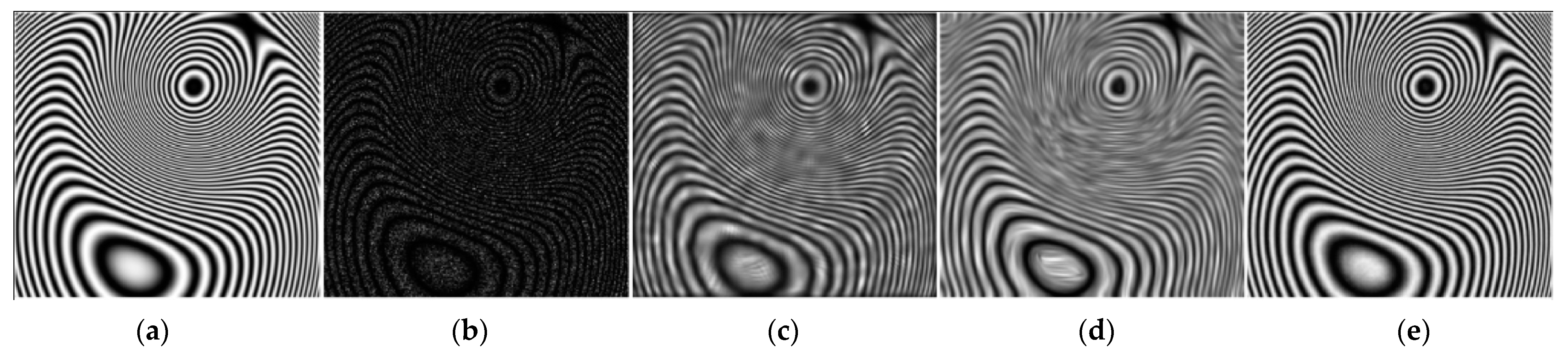
For (1), in 2019, Li et al. at Tianjin University proposed using the U-Net network for ESPI fringe skeleton line extraction [33]. This method treats skeleton line extraction as an image segmentation task from the background, successfully achieving skeleton line extraction. The method achieved an accuracy of 0.91 and a processing speed of 0.5 FPS and can extract different types of fringe skeleton lines with excellent generalization. However, this method performs poorly on fringe patterns with low contrast and considerable speckle noise. In 2022, the team improved on previous work by introducing the Channel-wise Cross Fusion Transformer into the U-Net network [34], which solved the problem of low accuracy. This method achieved an accuracy of 0.9878 and simultaneously performed phase extraction on the extracted fringe skeleton lines. Compared with conventional methods, the phase obtained by this method is smoother, and the performance regarding evaluation metrics is better, with an SSIM of 0.908 and root mean square error (RMSE) of 0.003. However, this method did not mention the average time for fringe extraction. Figure 7 displays a comparison of phase extraction results of various methods in the literature [34].
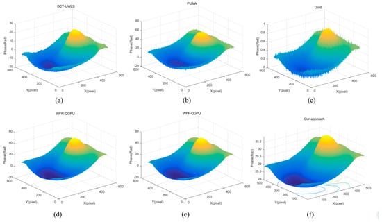
Figure 7.
Comparison of phase extraction results using different methods (a–f) show the methods of UWLS, Graphcut, Goldstein, WFR-QG, WFF-QG, and the literature [34], respectively).
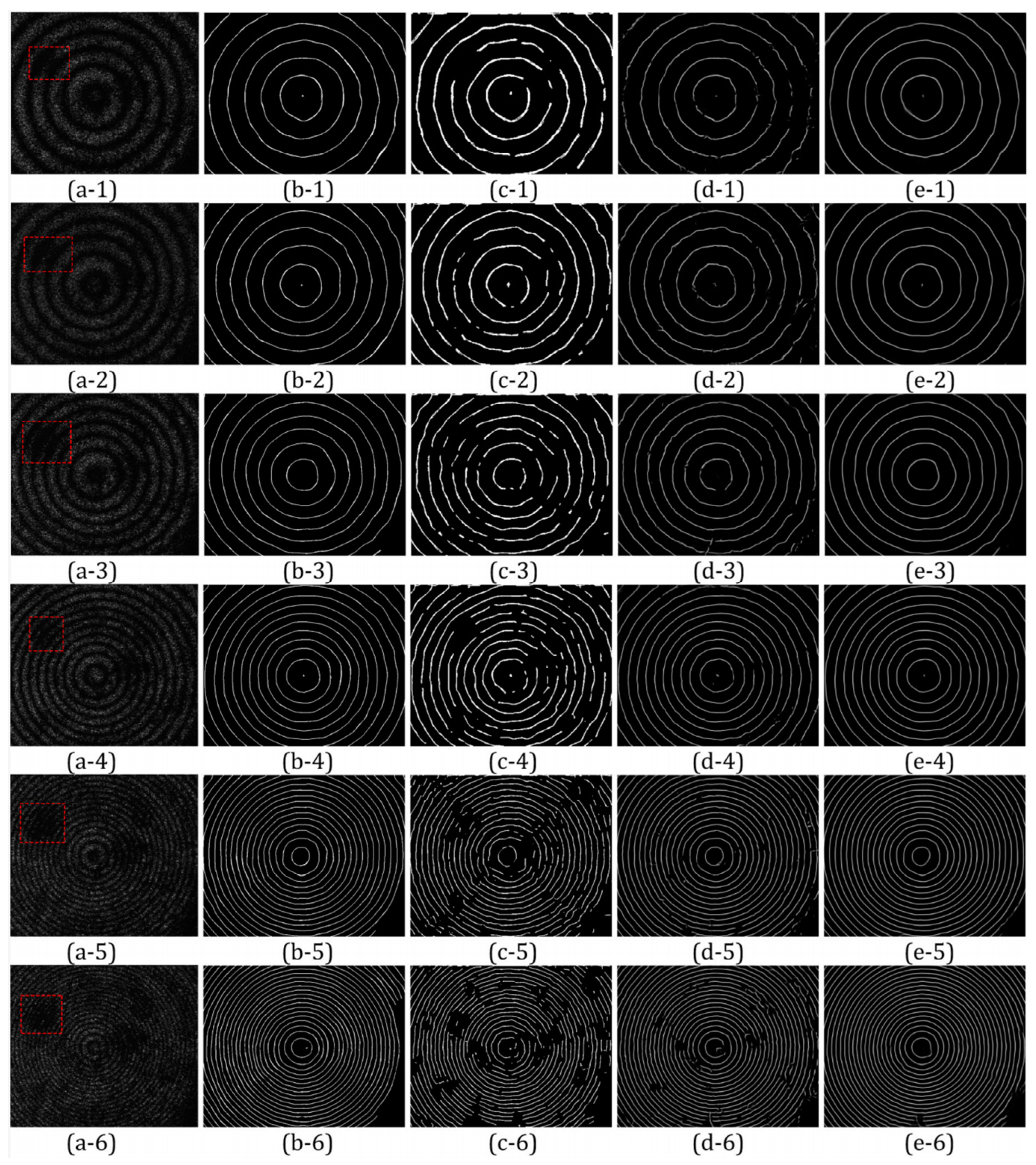
For problem (2), Liu et al. from Tianjin University proposed the M-Net network in 2020, which is an image segmentation task [35]. This method was used to analyze the experimental results obtained from the dynamic measurement of the thermal deformation of ceramic plates under strong light. Compared with conventional gradient vector field (VID-GVF) based on variational image decomposition [32] and U-Net [33] networks, M-Net achieved a superior extraction effect on the skeleton broken or missing stripes and can automatically fill in the damaged and broken parts. In terms of evaluation indicators, the accuracy, recall rate, and AUC score of the M-Net network were 0.959, 0.680, and 0.968, respectively, which were higher than those of VID-GVF (0.911, 0.531, and 0.735) and U-Net (0.952, 0.582, and 0.949). Figure 8 displays the specific experimental results, with red boxes representing damaged fringes.
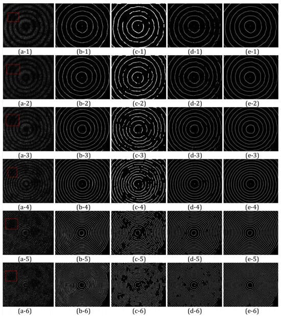
Figure 8.
Comparison of skeleton line extraction methods under thermal deformation of ceramic plates [35]. (a–e) Extracted skeleton lines using the measured fringe pattern and ideal skeleton line. (a-1–a-6) Input test images. (b-1–b-6) Ideal skeletons corresponding to the test images. (c-1–c-6) VID-GVF extraction method. (d-1–d-6) U-net extraction method. (e-1–e-6) M-Net extraction method. Red boxes represent damaged fringes.
At Hebei University of Technology, Wang et al. [36] considered skeleton line extraction as an image generation task. In the literature [36], Wang et al. used Pix2pix cGan [37] as a skeleton line extraction network, which can extract stripe skeleton lines and solve problem (1). This method is fast, reaching 11.7 FPS and an accuracy of 0.9704. Table 2 exhibits the comparison of the performance of five methods for extracting skeleton lines.
Table 2.
Comparison of the performance of five methods for extracting skeleton lines [32,33,34,35,36].
True Positive (TP): the number of samples that are actually positive and correctly predicted as positive.
True Negative (TN): the number of samples that are actually negative and correctly predicted as negative.
False Positive (FP): the number of samples that are actually negative but incorrectly predicted as positive.
False Negative (FN): the number of samples that are actually positive but incorrectly predicted as negative.
Existing deep learning methods have fewer applications in fringe skeleton line extraction, partly because the physical model for filtering denoising is more explicit, and more mature CNN models have been devised in other image processing fields, which can be directly imported into ESPI denoising. Most deep learning-based fringe skeleton line extraction methods add structural components in the encoder and decoder paths to adapt to ESPI fringe processing. Compared with the following methods, the previous method still requires specific algorithms for skeleton line extraction after filtering denoising, which increases the difficulty of fringe skeleton line extraction. Therefore, directly extracting fringe skeleton lines from the original fringe image without preprocessing could be the focus of research in the future.
3.3. Application of Deep Learning in the Interpolation Algorithm
The extracted fringe skeleton lines are discrete sampling points. To obtain the phase information of the entire field, an interpolation algorithm is required to predict the unsampled phase distribution of the entire field. Classic interpolation algorithms include bilinear interpolation [38], nearest neighbor interpolation [39], C spline interpolation [40], and interpolation methods based on the heat conduction theory [31]. Although these methods are simple and fast, they exhibit the following problems:
- (1)
- The interpolation result is not sufficiently accurate, and the resulting phase is not sufficiently smooth.
- (2)
- The quality requirements for the skeleton line are high.
- (3)
- Interpolation speed is slow.
Currently, the phase extraction interpolation algorithm for ESPI fringe patterns still relies on neural networks or simple machine learning methods, as the previous method displays in image format, whereas the subsequent one is related to mathematical methods.
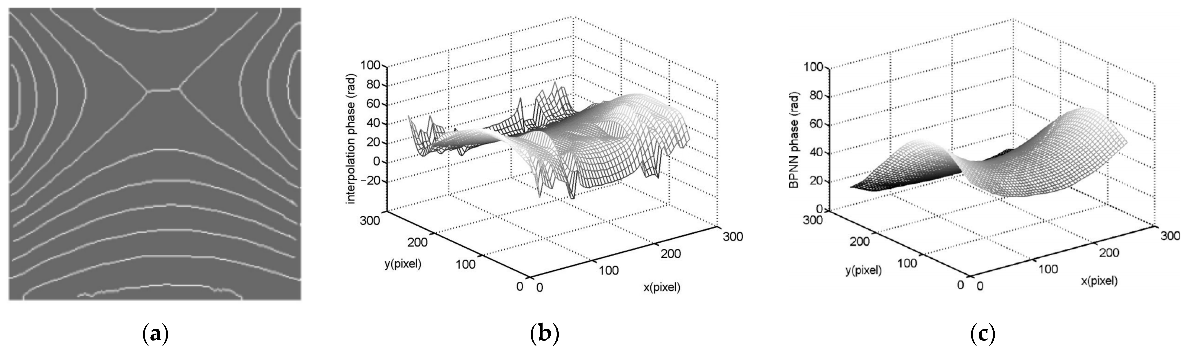
In 2007, Tang et al. at Tianjin University first proposed using a BP neural network for fringe skeleton line interpolation [41]. Figure 9 displays the results, which reveal that the phase information obtained by the network is smoother. However, this method requires specialized partial differential equation methods for preprocessing and lacks specific evaluation metrics to quantify the interpolation results. Determining the true phase accuracy obtained from the interpolated image alone is impossible.

Figure 9.
Interpolation results of different methods [41] (a–c) white striped skeleton line, C spline interpolation method ‘s result, and BPNN method’s result).
In 2011, Wang et al. from North China University of Technology proposed the radial basis function (RBF) neural network interpolation method, which solves the problem of high-quality requirements for skeleton lines and can obtain excellent results even for severely fractured skeleton lines [42]. However, similar to [41], specific quantitative metrics for evaluating the phase information obtained after interpolation were not provided. In addition, this method did not fully leverage the experimental data information from ESPI fringe patterns.
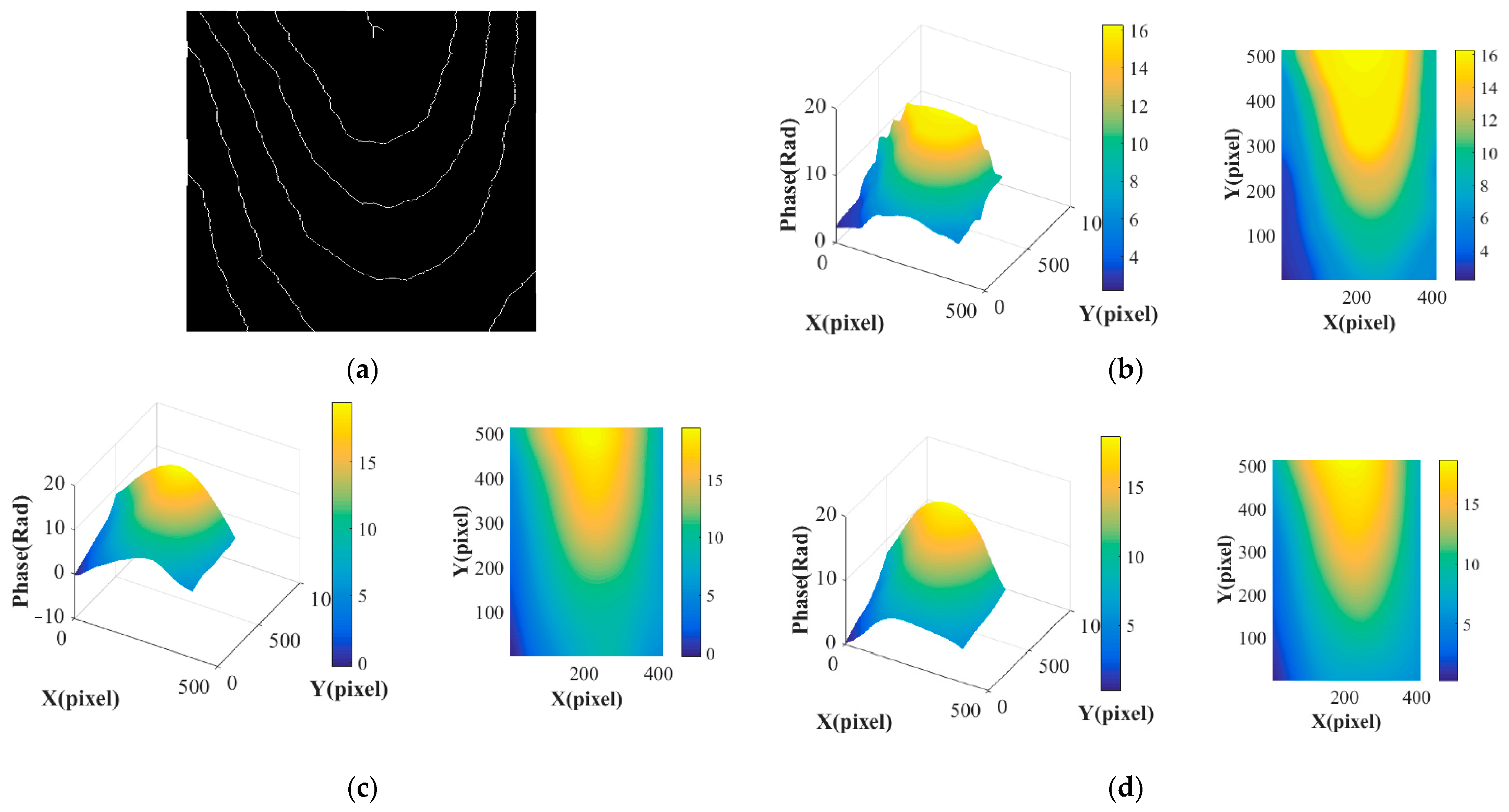
In 2020, Chen from Tianjin University proposed using hierarchical recurrent neural networks for interpolation processing, which solved the problem of slow processing speed [19]. In the thermal deformation experiment of steel plates under high-intensity laser irradiation, this method could perform interpolation operations on the fringe patterns obtained from dynamic measurements in only 4 s, which considerably lowered the 25 s required in the conventional method. Compared with the BP neural network method, the processing time of both methods was identical, but the phase information of the previous method was smoother. Figure 10 displays the specific interpolation results.

Figure 10.
Three-dimensional phase maps and two-dimensional pseudo-color phase maps interpolated using three different methods [19]. (a) Dynamic measurement fringe pattern of steel plate hot deformation. (b–d) Three-dimensional phase pattern and two-dimensional pseudo-color phase pattern from C-spline interpolation, a BP neural network, and reference [19], respectively.
Currently, interpolation algorithms have not been improved considerably, and the existing literature lacks quantitative evaluation metrics for phase information after interpolation. In this paper, because the evaluation of phase information only based on the smoothness of the image was inadequate, other evaluation metrics were required for quantification, For example, comparing the phase information after interpolation of classic methods with that based on neural network interpolation, calculating SSIM or RMSE between the two can make the performance comparison between methods more specific.
4. Application of Deep Learning in Phase Extraction of the ESPI-Wrapped Phase Image
Figure 11 displays the phase extraction method based on wrapped phase maps. The wrapped phase map is obtained using phase shifting, is then filtered and denoised, and finally unwrapped to obtain the final full-field phase information. The following sections describe the application of deep learning in the phase extraction of ESPI-wrapped phase maps.
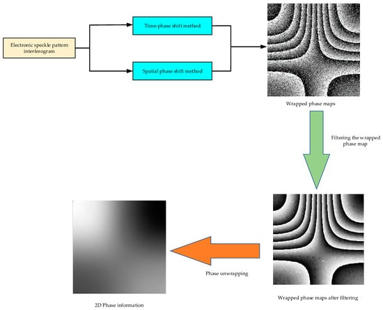
Figure 11.
Schematic of the phase extraction method based on the wrapped phase map [19].
4.1. Application of Deep Learning in the Phase Shift Method
According to the different methods of changing the phase difference, the classical phase shift method can be divided into the time phase shift and spatial phase shift method. The time phase shift method changes the phase shift amount on the time series to measure the deformation of the object and obtain deformation information. The spatial phase shift method obtains phase information by applying various phase shifts at one time. According to the different phase shift amounts, the three-step phase shift method [43], four-step phase shift method [44], five-step phase shift method [45], and so on have emerged successively. Their main difference is in the number of interferometric images used and the measurement accuracy. This article is focused on the most commonly used four-step phase shift algorithm. The four-step phase shift method collects four speckle patterns before and after object deformation, with a phase shift of 90° for each time in the speckle pattern collection. The intensity distribution of the four speckle interference patterns collected by the CCD can be expressed as follows:
Solving the above equations simultaneously, we can obtain the following phase of the optical field:
Improved four-step phase shift methods such as 4 + 2 [46] and 4 + 1 time phase shift techniques [47] have since emerged.
From a mathematical perspective, the classical phase shifting method involves adding a known phase shift under various conditions to increase the number of equations, rendering the number of equations greater than or equal to the unknowns, and subsequently solving for the phase value. When using conventional phase shifting methods for phase extraction, selecting an appropriate method based on the differences in processing objects and acquisition speed is necessary. In practice, the following problems are observed:
- (1)
- Conventional phase shifting requires the use of multiple images for phase extraction, whereas phase extraction based on a single fringe pattern exhibits lower accuracy. Balancing the two to achieve higher phase accuracy using fewer images remains challenging.
- (2)
- The process of time phase shifting requires the acquisition of multiple images, which requires considerable time and limits dynamic measurement.
In 2019, at the Nanjing University of Science and Technology, Feng et al. first demonstrated that deep neural networks can be trained to perform fringe analysis [48]. This study proposed a two-stage convolutional neural network. In the first network, the background intensity information in the fringe pattern was removed, and the output of the second network was the numerator and denominator of the arctangent function, as shown in Equation (17). Finally, the phase was calculated based on the output of network using the arctangent function. In this method, the phase was extracted using a single fringe pattern, and conventional phase shifting methods were combined to solve problem (1). The average absolute error of phase extraction using this method, Fourier transform (FT), and WFT was 0.087, 20, and 0.19 rad, respectively. Thus, the phase extraction accuracy improved considerably. However, this method requires the calculation of numerous accurate intermediate data from experimental data before training.
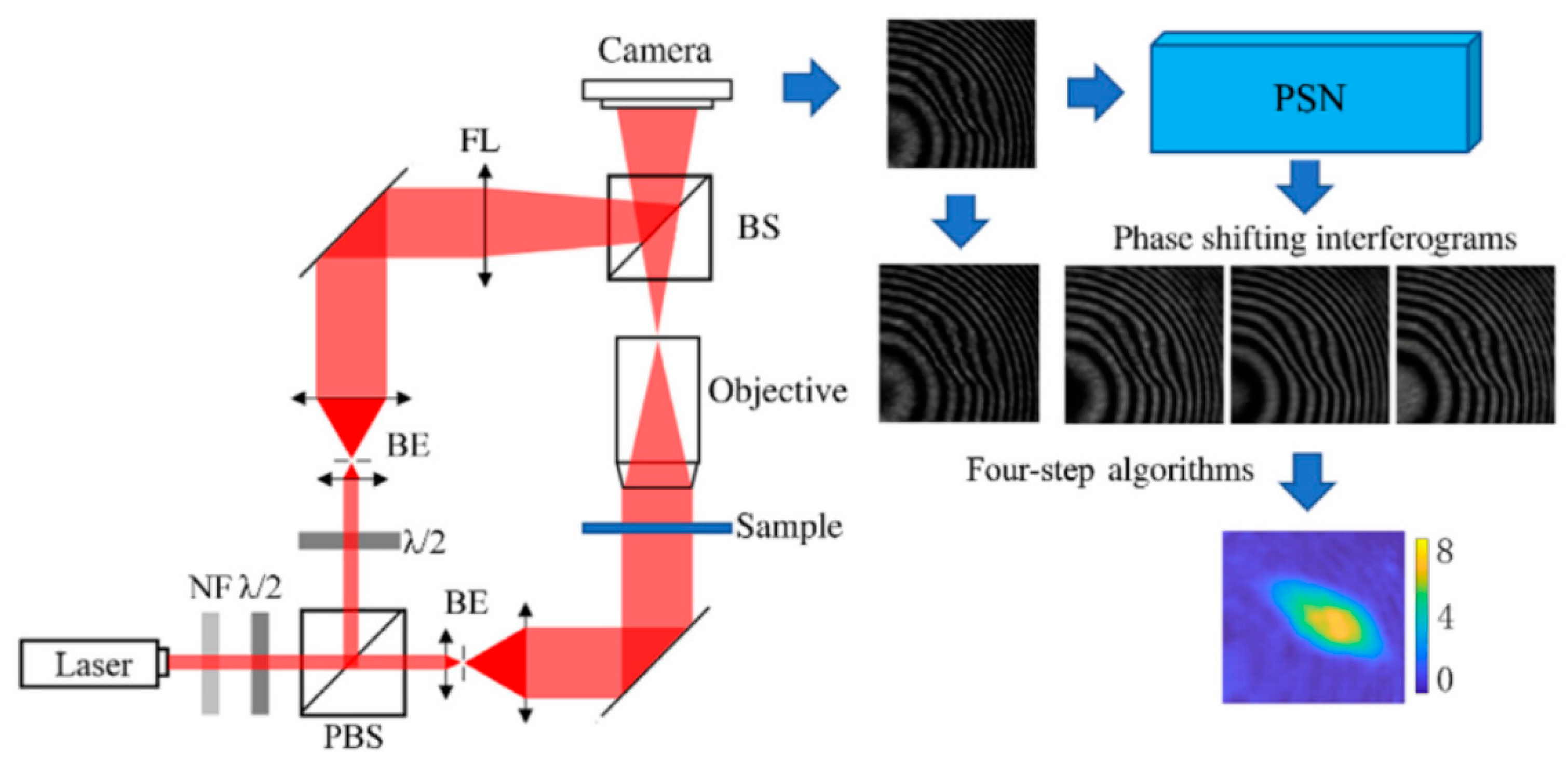
To solve problem (2), Zhang et al., at Shenzhen University, proposed a training strategy for phase shifting networks (PSNs) in 2021 [49]. The input of the method is a single frame of built-in interferogram, whereas the output comprises multiple phase shifting interferograms. This simulates the process of acquiring multiple images in conventional phase shifting. The speed of this method is only 65 ms, which is faster than the 160 ms of classic four-step phase shifting and slightly lower than the 30 ms of the single-frame interferogram phase extraction method. However, in terms of phase extraction RMSE, this method is only 0.11 rad, which is considerably lower than the 0.51 rad of the single-frame interferogram phase extraction method and close to the 0.09 rad of the classic four-step phase shifting. Figure 12 displays the specific method of reference [49].

Figure 12.
Method strategy from the literature [49].
4.2. Application of Deep Learning in ESPI-Wrapped Phase Image Filtering
The result obtained using the phase shifting method is an ESPI-wrapped phase map. The phase of the wrapped phase map is typically in the range and contains considerable noise. Therefore, filtering should be performed before applying the unwrapping algorithm to obtain the full-field phase. Compared with ESPI fringe filtering, the filtering of ESPI-wrapped phase maps mainly deals with noise and false phase jumps. Classic filtering methods include the module filtering method and the window Fourier filtering method based on convex optimization [19], but the following problems exist:
When severe noise is present in the ESPI-wrapped phase map, it leads to numerous false phase jumps. Conventional methods encounter challenges in handling false phase jumps during the denoising process, resulting in inaccurate unwrapping of denoised results.
- (1)
- Conventional filtering methods are time-consuming and require considerable parameter calculation.
- (2)
- Conventional methods have poor denoising capabilities for high-density and unevenly distributed phase maps.
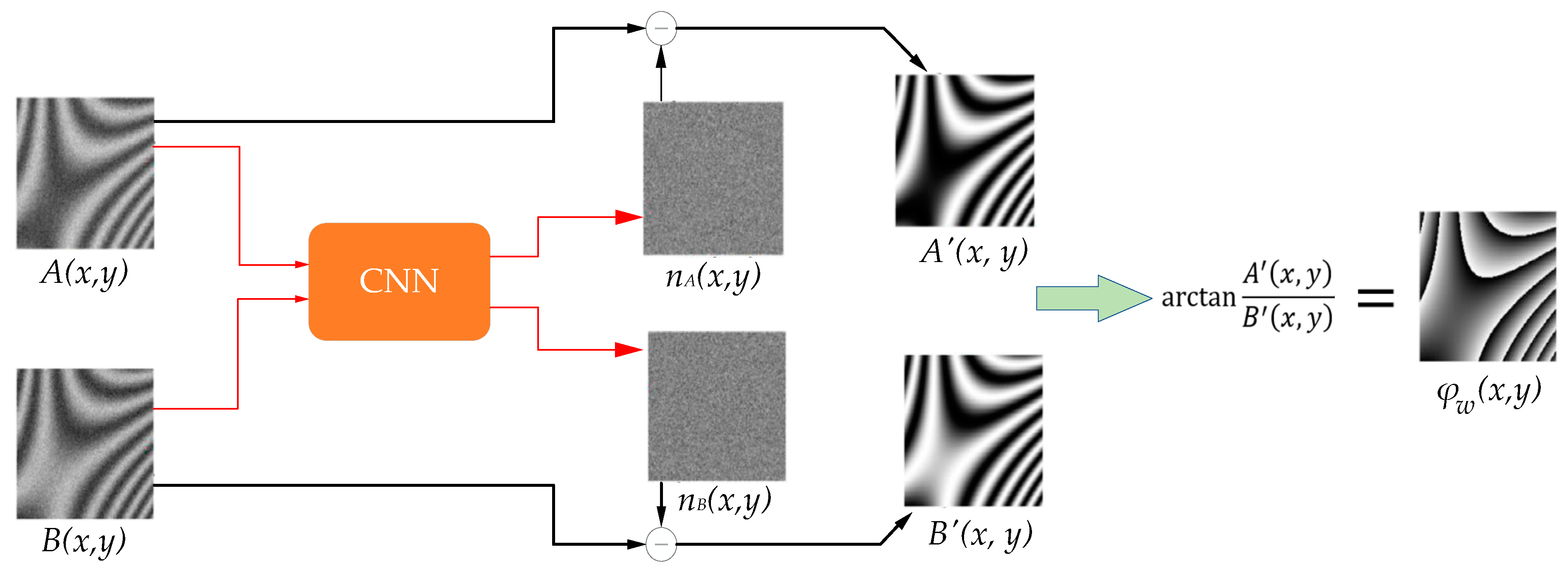
To solve problem (1), Yan et al. from Shanghai University and Nanyang Technological University in Singapore used CNN to denoise the numerator and denominator of the noisy arctan function and subsequently obtain a clear wrapped phase map using the denoised numerator and denominator [50]. This method can remove noise levels with an SNR of −4 dB at a speed of only 8.4 s. Furthermore, using this method to denoise the wrapped phase map for phase extraction, the RMSE increased with the increase in the phase frequency but was less than 0.055 rad. Figure 13 displays the specific method.
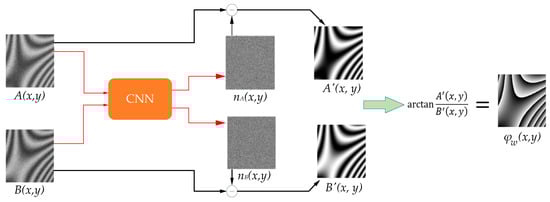
Figure 13.
Schematic of the denoising method proposed in [50]. Here, ( and are the results of and input into CNN, respectively).
To solve problem (2), in 2021, Tianjin University’s Li et al. introduced the DBDNet denoising network from other image denoising fields into the field of ESPI-wrapped phase map denoising [51]. The input of this network is the noisy wrapped phase map and the denoised phase map is the output, which theoretically reduces network parameters. Compared with conventional denoising methods OCPDE, WFLPF, and deep learning method FFD-Net, this method had a PSNR of 20.5648, which is significantly higher than the values of the previous three methods, 14.0865, 12.7554, and 17.3057, respectively. However, the method does not mention specific network calculation parameters. In subsequent work, the team improved and proposed a new network DBDNet2 in 2022 to solve problem (3) [52]. In ablation experiments, the denoising effect quantitative indexes (PSNR and SSIM) of this method were 19.1034 and 0.9078, respectively, which were higher than DBDNet’s 18.8819 and 0.8984, respectively. Table 3 summaries the ESPI package phase map-filtering methods based on deep learning.
Table 3.
Comparison of ESPI package phase map filtering methods based on deep learning [50,51,52].
Conventional ESPI image filtering methods and deep learning-based filtering methods have achieved considerable success, with their own advantages and disadvantages. Table 4 is a comparison of both methods.
Table 4.
Conventional and deep learning-based filtering methods.
Thus, conventional ESPI image filtering methods exhibit considerable advantages in physical model interpretability and algorithm simplicity, whereas deep learning methods have advantages in adaptability and handling complex relationships. Therefore, for datasets in various application scenarios, appropriate methods should be selected according to the needs.
4.3. Application of Deep Learning in the Phase Unwrapping Algorithm
The phase distribution obtained after the phase shifting process is typically encapsulated in an arctangent function, as shown in Formula (17). This phase distribution is wrapped, that is, the phase value only changes within the range . This is a discontinuous phase distribution that does not match the true phase distribution. To obtain continuous and meaningful phase information, a phase unwrapping operation is required. Phase unwrapping is the process of unfolding the wrapped speckle phase into a continuous phase distribution to eliminate the periodic accumulation of phases, rendering the phase continuous and meaningful throughout the domain.
Currently, phase unwrapping methods based on deep learning can be classified into two categories, namely image segmentation-based methods and one-step direct unwrapping methods. “Segmentation” denotes determining the addition of two unknown integral multiples at each pixel in the wrapped phase to recover the true phase. One-step direct unwrapping methods learn the feature mapping between the wrapped phase map and the unwrapped image through convolutional networks.
4.3.1. Unwrapping Algorithm Based on Image Segmentation
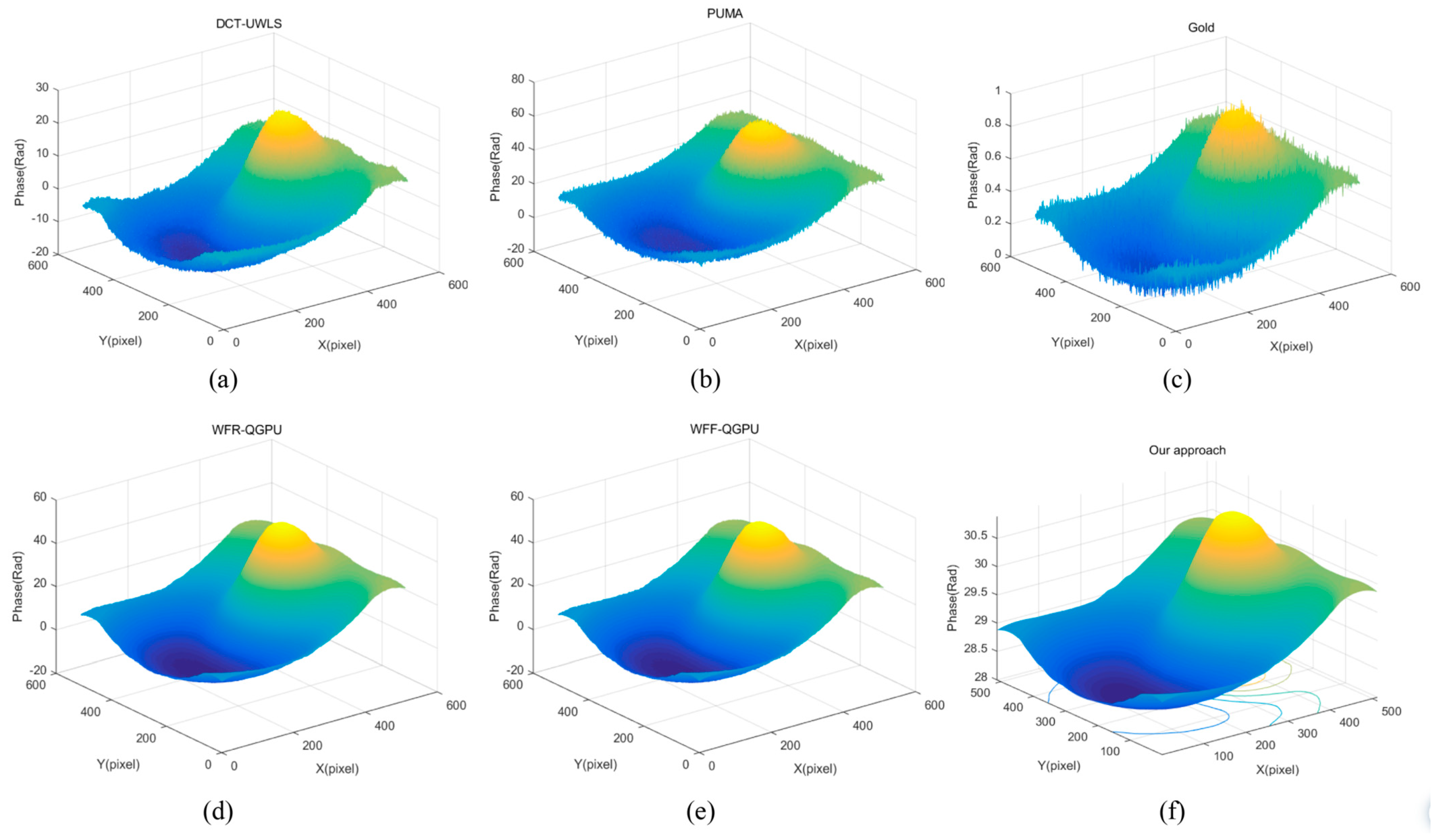
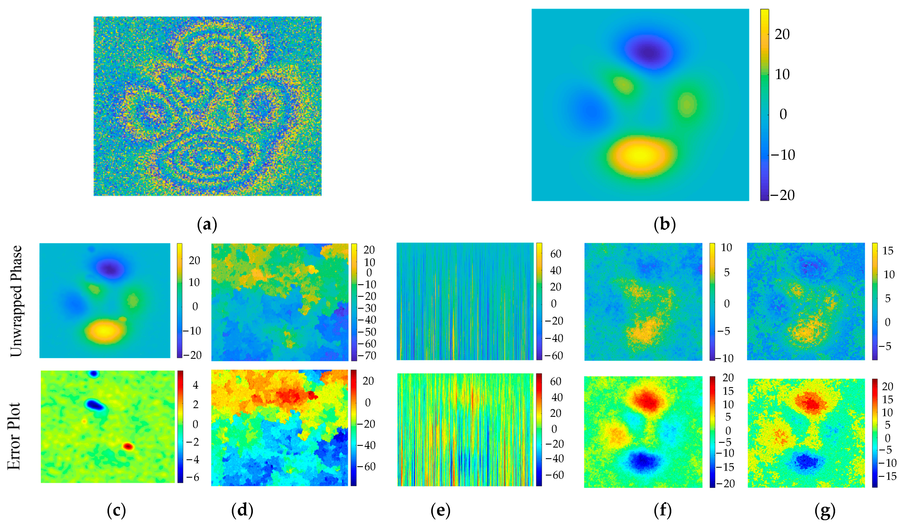
In some cases, phase unwrapping is considered an image segmentation task. In 2018, G.E. Spoorthi et al. [53] of the Indian Institute of Technology proposed the deep learning phase unwrapping framework PhaseNet. Compared with the unwrap function in MATLAB and the quality-guided phase unwrap method (QGPU), PhaseNet has a phase MSE of 2 and a time cost of 0.18 s at an SNR of 0 dB, which is considerably better than the values obtained by the unwrap function (11 and 24 s for phase MSE and time cost, respectively) and QGPU (17 and 0.05 s, respectively). However, this method requires post-processing steps and can only unwrap phases within the range −36 to +36 radians. In 2020, the team proposed PhaseNet2.0, which increased the unwrapping range to 100 radians and eliminated the necessity for post-processing in PhaseNet [54]. Compared to QGPU, MATLAB unwrap function, least square phase unwrapping (LSPU), and calibrated least square phase unwrapping (CLSPU) methods, PhaseNet2.0 unwraps phases more smoothly on the image, with root mean square of 2.5%, which is significantly better than the values of 178.2%, 85.6%, 24.3%, and 26.3%, respectively, obtained by the former methods. Figure 14 displays the specific unwrapping effect.
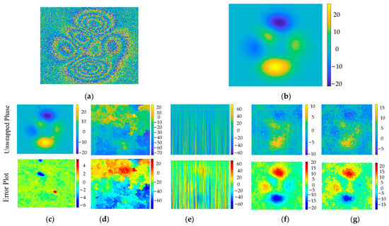
Figure 14.
Comparison of the unwrapping phase method in reference [54] to other methods. (a) Wrapped phase at SNR = −4 dB. (b) Ground truth. (c) Reference [54]’s method. Qualitative analysis of the proposed method at SNR = −4 dB compared to (d) quality-guided phase unwrapping (QGPU), (e) MATLAB’s unwrap function, (f) least square phase unwrapping (LSPU), and (g) calibrated least square phase unwrapping (CLSPU).
Similarly, considering phase unwrapping as an image segmentation task, in 2019, Zhang et al. from Hangzhou Dianzi University used an extended DeepLabV3+ network as the backbone to solve the problem of conventional methods being prone to failure in high-noise datasets [55]. Using a Gaussian white noise dataset for phase unwrapping, the RMSE of this method is 1.2325, demonstrating considerably superior unwrapping performance compared with the conventional path-following method with an RMSE of 19.7591. In 2019, Zhang et al. from Shenyang Institute of Automation of the Chinese Academy of Sciences and the School of Optical Sciences of the University of Arizona in the United States combined CNN denoising network and CNN segmentation network to improve performance [56]. The RMSE of this method is only 0.0027, and the processing speed of the GPU is 0.22 s, which is significantly better than 6.5202 and 19.53 s of the branch cutting algorithm, and 6.2683 and 330.44 s of the QGPU method, respectively.
4.3.2. One-Step Direct Unwrapping Algorithm
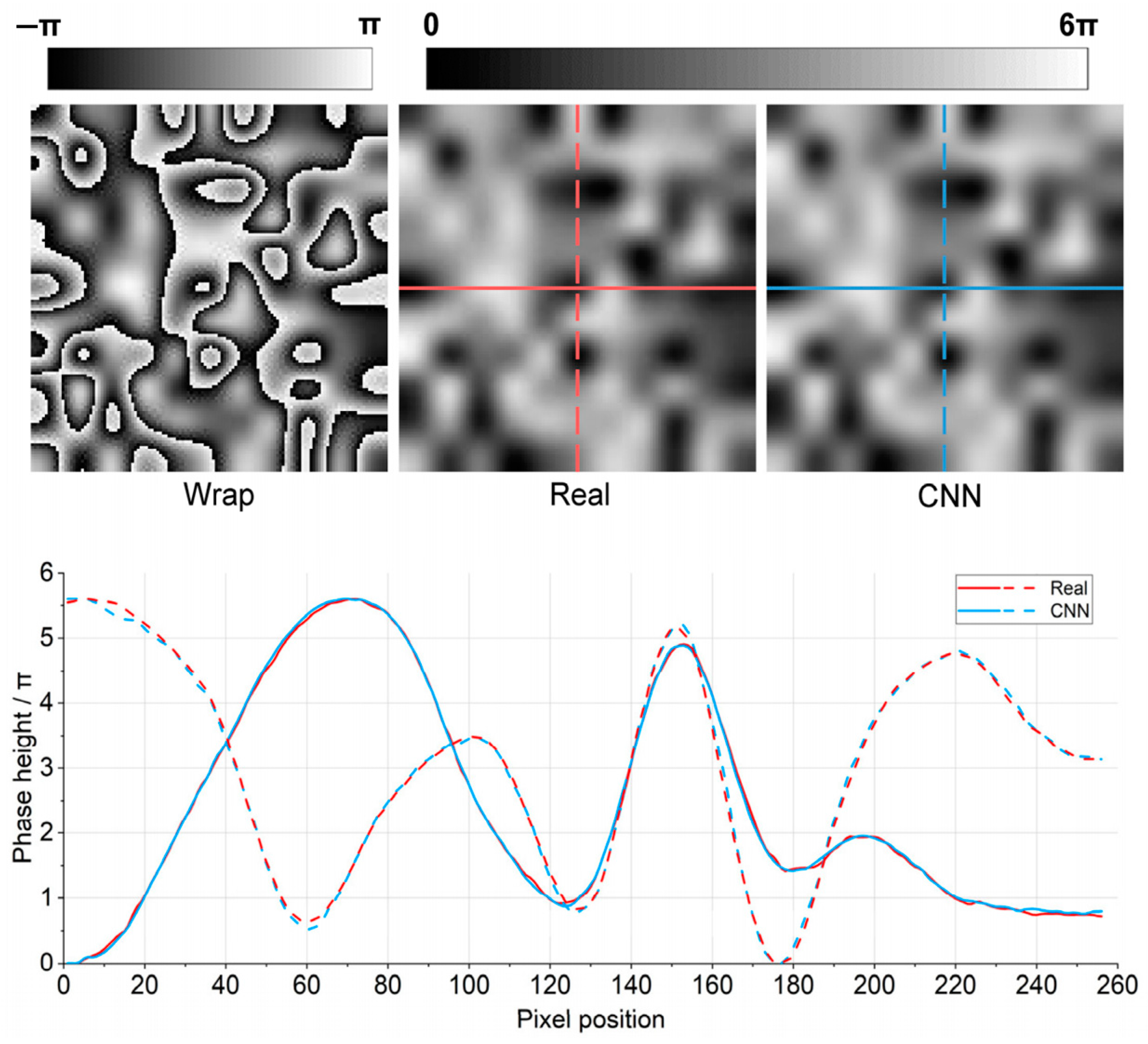
Another group of scholars considered the one-step unwrapping method. In 2019, at the Northwestern Polytechnical University, Wang et al. introduced Residual Block into the U-Net network and proposed a one-step unwrapping method deep learning phase unwrapping (DLPU) [57], as displayed in Figure 15. The SSIM of the phase-unwrapped image and the reference image reached 0.991. In terms of robustness, compared with the least squares (LS) method and the quality guidance (QG) method, when the true phase height increased from 5 to 100, the SSIM index of DLPU decreased from 0.99 to 0.80, which was significantly better than those LS and QG methods (down to 0.2). The maximum error pixel ratio of DLPU is 0.2, which is 3.55 times lower than the ratios of the LS and QG methods (0.71). Subsequently, at the Beijing University of Technology in 2020, Qin et al. were inspired by VGG, U-Net, and ResNet, and proposed the VUR-Net method [58]. Xu et al. from Tianjin University [59] considered reducing the computational burden when improving the accuracy of phase unwrapping and proposed the PU-M-Net method. This approach effectively reduced speckles during the phase unwrapping process. On a high-noise dataset, PU-M-Net achieved an SSIM of 0.810 and MSE of 1.673, outperforming the LS method with 6.870 and 0.562, as well as the QGPU method with 2.585 and 0.771, respectively. Table 5 compares all the deep learning-based unwrapping methods mentioned above.
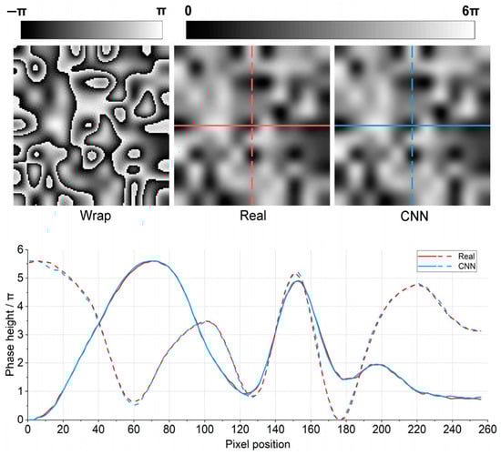
Figure 15.
Comparison of the DLPU method unwrapping and phase method [57]. Upper row: the wrapped, real and CNN-output unwrapped phase images; Lower row: the comparison of phase height across the central lines indicated in real phase (red lines) and CNN-output unwrapped phase (blue lines).
Table 5.
Summary of unwrapping methods based on deep learning [53,54,55,56,57,58,59].
Based on the analysis, phase unwrapping methods based on image segmentation usually use simple networks and require preprocessing or post-processing to obtain reliable results. However, one-step direct unwrapping methods use more complex networks and can directly obtain reliable results.
Compared with conventional unwrapping algorithms, deep learning-based unwrapping methods exhibit a strong generalization ability, fast processing speed, and accurate phase information. However, these methods still require a large-scale dataset. Therefore, improving the accuracy and feature extraction efficiency of the network as well as reducing the requirements of the dataset are problems that need to be addressed in the current research. Addressing dataset requirements while achieving one-step direct unwrapping of the phase with high accuracy becomes a prominent topic in this field.
5. Summary and Outlook
Compared with conventional methods of phase extraction from electronic speckle interferometric images, deep learning methods have demonstrated advancements in terms of accuracy, processing speed, and generalization. Research in this field is still in its nascent stages, and several promising avenues warrant in-depth exploration:
- (1)
- Integration of the physical model into the deep learning model.
The generation mechanism of ESPI images is well understood, whereas deep learning models are considered “black boxes” with challenging internal mechanisms. Integrating prior knowledge with the mature generation process of ESPI images into deep learning models for different application scenarios can become a novel research direction for developing new data-driven deep learning models.
- (2)
- Improvement and optimization of deep learning models.
Most existing deep learning models focus on the classical models such as CNN and their enhancements. With the continuous development of deep learning technology, novel models are expected to emerge. In the next phase, investigating the application of various models to phase extraction in electronic speckle interferometric images is crucial. Moreover, existing deep learning models are limited to specific steps in the phase extraction process and lack an end-to-end complete model. Therefore, introducing new deep learning models and constructing end-to-end phase extraction models will become a prominent research direction in the future.
- (3)
- Quantitative evaluation of phase extraction quality.
Existing phase extraction methods based on deep learning models are typically applied to specific steps, such as filtering and fringe skeleton extraction. Evaluation metrics for the algorithm are confined to these intermediate steps, without focusing on the quality of phase extraction. This renders the quantitative evaluation and comparative analysis of phase extraction quality challenging. Therefore, addressing the urgent need for a quantitative evaluation of phase extraction quality is essential.
- (4)
- Limited practical engineering applications.
At present, the ESPI phase extraction method based on deep learning is in its early stage of development, and thus is mainly only applied in the laboratory. There are only a few notable applications of these algorithms outside the laboratory, and there are currently very few practical applications in the field of industrial engineering. The application of deep learning methods to ESPI phase extraction has great potential in industrial engineering and other fields. This application may result in more efficient and accurate phase extraction methods and provide better support for industrial applications in related fields.
- (5)
- Expanding the dataset.
Currently, limited publicly available ESPI image datasets are available in the industry, hindering the validation of the practical generalization ability of deep learning models and impeding meaningful horizontal comparisons between research outcomes. In the next step, studies should focus on generating ESPI image datasets through numerical simulation and constructing experimental systems in conjunction with practical application scenarios. A comprehensive analysis of factors influencing image quality and further dataset expansion is essential.
Author Contributions
Conceptualization, W.J. and T.R.; methodology, T.R. and Q.F.; validation, W.J. and T.R.; data curation, W.J. and T.R.; investigation, T.R. and Q.F.; writing—original draft preparation, T.R. and Q.F.; writing—review and editing, W.J.; supervision, W.J.; funding acquisition, W.J. All authors have read and agreed to the published version of the manuscript.
Funding
This work was supported by Sichuan Science and Technology Program, under grant no. 2021JDJQ0027, and the Natural Science Foundation of China, under grant no. 61875166.
Data Availability Statement
The data underlying the results presented in this paper are not publicly available at this time but may be obtained from the authors upon reasonable request.
Acknowledgments
Wenbo Jiang would like to acknowledge the Sichuan Provincial Academic and Technical Leader Training Plan, and the Overseas Training Plan of Xihua University (09/2014-09/2015, University of Michigan, Ann Arbor, US). We would also like to thank LetPub (www.letpub.com accessed on 15 January 2024) for its linguistic assistance and scientific consultation during the preparation of this manuscript.
Conflicts of Interest
The authors declare no conflicts of interest.
References
- Vaz, B.F.; Ferracini, E.; Santos, A.A.; Gonçalves, R. Measuring stress fields in connecting rods using laser interferometry (ESPI). J. Test. Eval. 2015, 43, 735–748. [Google Scholar] [CrossRef]
- Martínez, A.; Rayas, J.A.; Rodríguez-Vera, R.; Puga, H.J. Three-dimensional deformation measurement from the combination of in-plane and out-of-plane electronic speckle pattern interferometers. Appl. Opt. 2004, 43, 4652–4658. [Google Scholar] [CrossRef] [PubMed]
- Nitta, I.; Sato, T.; Tsukiyama, Y. 3D surface profile measurement by single shot interferometry with wide field of view. In Proceedings of the Asian Conference on Experimental Mechanics, Niigata City, Japan, 7–10 October 2019. [Google Scholar]
- Kumar, M.; Gaur, K.K.; Shakher, C. Measurement of material constants (Young’s modulus and Poisson’s ratio) of polypropylene using digital speckle pattern interferometry (DSPI). J. Jpn. Soc. Exp. Mech. 2015, 15, s87–s91. [Google Scholar]
- Kennedy, D.M.; Schauperl, Z.; Greene, S. Application of ESPI-method for strain analysis in thin wall cylinders. Opt. Lasers Eng. 2004, 41, 585–594. [Google Scholar] [CrossRef]
- Labbe, F. Strain-rate measurements by electronic speckle-pattern interferometry (ESPI). Opt. Lasers Eng. 2007, 45, 827–833. [Google Scholar] [CrossRef]
- Loukil, M.S.; Ayadi, Z.; Varna, J. ESPI analysis of crack face displacements in damaged laminates. Compos. Sci. Technol. 2014, 94, 80–88. [Google Scholar] [CrossRef]
- Yang, L.; Xie, X.; Zhu, L.; Wu, S.; Wang, Y. Review of electronic speckle pattern interferometry (ESPI) for three dimensional displacement measurement. Chin. J. Mech. Eng. 2014, 27, 1–13. [Google Scholar] [CrossRef]
- Shuhai, J.; Kaiduan, Y.; Yushan, T. The system of double-optical-path ESPI for the vibration measurement. Opt. Lasers Eng. 2000, 34, 67–74. [Google Scholar] [CrossRef]
- Farrant, D.I.; Petzing, J.N.; Tyrer, J.R. Geometrically qualified ESPI vibration analysis of an engine. Opt. Lasers Eng. 2004, 41, 659–671. [Google Scholar] [CrossRef]
- Li, X.; Sung, P.; Patterson, E.; Wang, W.; Christian, W. Identification of defects in composite laminates by comparison of mode shapes from electronic speckle pattern interferometry. Opt. Lasers Eng. 2023, 163, 107444. [Google Scholar] [CrossRef]
- Ferretti, D.; Rossi, M.; Royer-Carfagni, G. An ESPI experimental study on the phenomenon of fracture in glass. Is it brittle or plastic? J. Mech. Phys. Solids 2011, 59, 1338–1354. [Google Scholar] [CrossRef]
- Wang, K.; Song, L.; Wang, C.; Ren, Z.; Zhao, G.; Dou, J.; Di, J.; Barbastathis, G.; Zhou, R.; Zhao, J.; et al. On the use of deep learning for phase recovery. Light Sci. Appl. 2024, 13, 4. [Google Scholar] [CrossRef] [PubMed]
- Zuo, C.; Feng, S.; Huang, L.; Tao, T.; Yin, W.; Chen, Q. Phase shifting algorithms for fringe projection profilometry: A review. Opt. Lasers Eng. 2018, 109, 23–59. [Google Scholar] [CrossRef]
- de Groot, P. Phase-shift calibration errors in interferometers with spherical Fizeau cavities. Appl. Opt. 1995, 34, 2856–2863. [Google Scholar] [CrossRef] [PubMed]
- LeCun, Y.; Bengio, Y.; Hinton, G. Deep learning. Nature 2015, 521, 436–444. [Google Scholar] [CrossRef] [PubMed]
- Zuo, C.; Qian, J.; Feng, S.; Yin, W.; Li, Y.; Fan, P.; Han, J.; Qian, K.; Chen, Q. Deep learning in optical metrology: A review. Light Sci. Appl. 2022, 11, 39. [Google Scholar] [CrossRef] [PubMed]
- Archbold, E.; Burch, J.M.; Ennos, A.E.; Taylor, P.A. Visual observation of surface vibration nodal patterns. Nature 1969, 222, 263–265. [Google Scholar] [CrossRef]
- Chen, M. Research and Application of A New Method for Phase Extraction in Electronic Speckle Interferometry Based on Machine Learning. Ph.D. Thesis, Tianjin University, Tianjin, China, 2020. (In Chinese). [Google Scholar]
- Tang, C.; Han, L.; Ren, H.; Zhou, D.; Chang, Y.; Wang, X.; Cui, X. Second-order oriented partial-differential equations for denoising in electronic-speckle-pattern interferometry fringes. Opt. Lett. 2008, 33, 2179–2181. [Google Scholar] [CrossRef]
- Zhang, K.; Zuo, W.; Zhang, L. FFDNet: Toward a fast and flexible solution for CNN-based image denoising. IEEE Trans. Image Process. 2018, 27, 4608–4622. [Google Scholar] [CrossRef]
- Hao, F.; Tang, C.; Xu, M.; Lei, Z. Batch denoising of ESPI fringe patterns based on convolutional neural network. Appl. Opt. 2019, 58, 3338–3346. [Google Scholar] [CrossRef]
- Lin, B.; Fu, S.; Zhang, C.; Wang, F.; Li, Y. Optical fringe patterns filtering based on multi-stage convolution neural network. Opt. Lasers Eng. 2020, 126, 105853. [Google Scholar] [CrossRef]
- Wang, L.; Li, R.; Tian, F.; Fang, X. Application of attention-DnCNN for ESPI fringe patterns denoising. J. Opt. Soc. Am. A Opt. Image Sci. Vis. 2022, 39, 2110–2123. [Google Scholar] [CrossRef] [PubMed]
- Xu, M.; Tang, C.; Hong, N.; Lei, Z. MDD-Net: A generalized network for speckle removal with structure protection and shape preservation for various kinds of ESPI fringe patterns. Opt. Lasers Eng. 2022, 154, 107017. [Google Scholar] [CrossRef]
- Gurrola-Ramos, J.; Dalmau, O.; Alarcon, T. U-Net based neural network for fringe pattern denoising. Opt. Lasers Eng. 2022, 149, 106829. [Google Scholar] [CrossRef]
- Lam, L.; Lee, S.W.; Suen, C.Y. Thinning methodologies a comprehensive survey. IEEE Trans. Pattern Anal. Mach. Intell. 1992, 14, 869–885. [Google Scholar] [CrossRef]
- Quan, C.; Tay, C.J.; Yang, F.; He, X. Phase extraction from a single fringe pattern based on guidance of an extreme map. Appl. Opt. 2005, 44, 4814–4821. [Google Scholar] [CrossRef] [PubMed]
- Tang, C.; Lu, W.; Cai, Y.; Han, L.; Wang, G. Nearly preprocessing-free method for skeletonization of gray-scale electronic speckle pattern interferometry fringe patterns via partial differential equations. Opt. Lett. 2008, 33, 183–185. [Google Scholar] [CrossRef]
- Tang, C.; Ren, H.; Wang, L.; Wang, Z.; Han, L.; Gao, T. Oriented couple gradient vector fields for skeletonization of gray-scale optical fringe patterns with high density. Appl. Opt. 2010, 49, 2979–2984. [Google Scholar] [CrossRef]
- Zhang, F.; Wang, D.; Xiao, Z.; Geng, L.; Wu, J.; Xu, Z.; Sun, J.; Wang, J.; Xi, J. Skeleton extraction and phase interpolation for single ESPI fringe pattern based on the partial differential equations. Opt. Express 2015, 23, 29625–29638. [Google Scholar] [CrossRef]
- Chen, X.; Tang, C.; Li, B.; Su, Y. Gradient vector fields based on variational image decomposition for skeletonization of electronic speckle pattern interferometry fringe patterns with variable density and their applications. Appl. Opt. 2016, 55, 6893–6902. [Google Scholar] [CrossRef]
- Li, B.; Tang, C.; Zheng, T.; Lei, Z. Fully automated extraction of the fringe skeletons in dynamic electronic speckle pattern interferometry using a U-Net convolutional neural network. Opt. Eng. 2019, 58, 023105. [Google Scholar] [CrossRef]
- Li, B.; Li, Z.; Zhang, J.; Sun, G.; Mei, J.; Yan, J. Channel transformer U-Net: An automatic and effective skeleton extraction network for electronic speckle pattern interferometry. Appl. Opt. 2023, 62, 325–334. [Google Scholar] [CrossRef] [PubMed]
- Liu, C.; Tang, C.; Xu, M.; Hao, F.; Lei, Z. Skeleton extraction and inpainting from poor, broken ESPI fringe with an M-net convolutional neural network. Appl. Opt. 2020, 59, 5300–5308. [Google Scholar] [CrossRef] [PubMed]
- Wang, H.; Zhang, Z.; Zhu, Q.; Wang, X.; Dong, Z.; Men, G.; Wang, J.; Lei, J.; Wang, W. Batch skeleton extraction from ESPI fringe patterns using pix2pix conditional generative adversarial network. Opt. Rev. 2022, 29, 97–105. [Google Scholar] [CrossRef]
- Isola, P.; Zhu, J.Y.; Zhou, T.; Efros, A.A. Image-to-image translation with conditional adversarial networks. In Proceedings of the 2017 IEEE Conference on Computer Vision and Pattern Recognition (CVPR), Honolulu, HI, USA, 21–27 July 2017; pp. 5967–5976. [Google Scholar]
- Parker, J.A.; Kenyon, R.V.; Troxel, D.E. Comparison of interpolating methods for image resampling. IEEE Trans. Med. Imaging 1983, 2, 31–39. [Google Scholar] [CrossRef] [PubMed]
- Lehmann, T.M.; Gonner, C.; Spitzer, K. Survey: Interpolation methods in medical image processing. IEEE Trans. Med. Imaging 1999, 18, 1049–1075. [Google Scholar] [CrossRef] [PubMed]
- Maeland, E. On the comparison of interpolation methods. IEEE Trans. Med. Imaging 1988, 7, 213–217. [Google Scholar] [CrossRef]
- Tang, C.; Lu, W.; Chen, S.; Zhang, Z.; Li, B.; Wang, W.; Han, L. Denoising by coupled partial differential equations and extracting phase by backpropagation neural networks for electronic speckle pattern interferometry. Appl. Opt. 2007, 46, 7475–7484. [Google Scholar] [CrossRef]
- Wang, G.; Li, Y.J.; Zhou, H.C. Application of the radial basis function interpolation to phase extraction from a single electronic speckle pattern interferometric fringe. Appl. Opt. 2011, 50, 3110–3117. [Google Scholar] [CrossRef]
- Huang, P.S.; Zhang, S. Fast three-step phase-shifting algorithm. Appl. Opt. 2006, 45, 5086–5091. [Google Scholar] [CrossRef]
- Schwider, J.; Falkenstoerfer, O.R.; Schreiber, H.; Zoeller, A.; Streibl, N. New compensating four-phase algorithm for phase-shift interferometry. Opt. Eng. 1993, 32, 1883–1885. [Google Scholar] [CrossRef]
- Novak, J. Five-step phase-shifting algorithms with unknown values of phase shift. Optik 2003, 114, 63–68. [Google Scholar] [CrossRef]
- Ponslet, E.; Steinzig, M. Residual stress measurement using the hole drilling method and laser speckle interferometry part III: Analysis technique. Exp. Tech. 2003, 27, 45–48. [Google Scholar] [CrossRef]
- Bi, H.; Zhang, Y.; Ling, K.V.; Wen, C. Class of 4 + 1-phase algorithms with error compensation. Appl. Opt. 2004, 43, 4199–4207. [Google Scholar] [CrossRef] [PubMed]
- Feng, S.; Chen, Q.; Gu, G.; Tao, T.; Zhang, L.; Hu, Y.; Yin, W.; Zuo, C. Fringe pattern analysis using deep learning. Adv. Photonics 2019, 1, 025001. [Google Scholar] [CrossRef]
- Zhang, Q.; Lu, S.; Li, J.; Li, D.; Lu, X.; Zhong, L.; Tian, J. Phase-shifting interferometry from single frame in-line interferogram using deep learning phase-shifting technology. Opt. Commun. 2021, 498, 127226. [Google Scholar] [CrossRef]
- Yan, K.; Yu, Y.; Sun, T.; Asundi, A.; Kemao, Q. Wrapped phase denoising using convolutional neural networks. Opt. Lasers Eng. 2020, 128, 105999. [Google Scholar] [CrossRef]
- Li, J.; Tang, C.; Xu, M.; Fan, Z.; Lei, Z. DBDNet for denoising in ESPI wrapped phase patterns with high density and high speckle noise. Appl. Opt. 2021, 60, 10070–10079. [Google Scholar] [CrossRef]
- Li, J.; Tang, C.; Xu, M.; Lei, Z. Uneven wrapped phase pattern denoising using a deep neural network. Appl. Opt. 2022, 61, 7150–7157. [Google Scholar] [CrossRef]
- Spoorthi, G.E.; Gorthi, S.; Gorthi RK, S.S. PhaseNet: A deep convolutional neural network for two-dimensional phase unwraping. IEEE Signal Process. Lett. 2018, 26, 54–58. [Google Scholar] [CrossRef]
- Spoorthi, G.E.; Gorthi RK, S.S.; Gorthi, S. PhaseNet 2.0: Phase unwrapping of noisy data based on deep learning approach. IEEE Trans. Image Process. 2020, 29, 4862–4872. [Google Scholar] [CrossRef]
- Zhang, T.; Jiang, S.; Zhao, Z.; Dixit, K.; Zhou, X.; Hou, J.; Zhang, Y.; Yan, C. Rapid and robust two-dimensional phase unwrapping via deep learning. Opt. Express 2019, 27, 23173–23185. [Google Scholar] [CrossRef] [PubMed]
- Zhang, J.; Tian, X.; Shao, J.; Luo, H.; Liang, R. Phase unwrapping in optical metrology via denoised and convolutional segmentation networks. Opt. Express 2019, 27, 14903–14912. [Google Scholar] [CrossRef] [PubMed]
- Wang, K.; Li, Y.; Kemao, Q.; Di, J.; Zhao, J. One-step robust deep learning phase unwrapping. Opt. Express 2019, 27, 15100–15115. [Google Scholar] [CrossRef]
- Qin, Y.; Wan, S.; Wan, Y.; Weng, J.; Liu, W.; Gong, Q. Direct and accurate phase unwrapping with deep neural network. Appl. Opt. 2020, 59, 7258–7267. [Google Scholar] [CrossRef]
- Xu, M.; Tang, C.; Shen, Y.; Hong, N.; Lei, Z. PU-M-Net for phase unwrapping with speckle reduction and structure protection in ESPI. Opt. Lasers Eng. 2022, 151, 106824. [Google Scholar] [CrossRef]


Disclaimer/Publisher’s Note: The statements, opinions and data contained in all publications are solely those of the individual author(s) and contributor(s) and not of MDPI and/or the editor(s). MDPI and/or the editor(s) disclaim responsibility for any injury to people or property resulting from any ideas, methods, instructions or products referred to in the content. |
© 2024 by the authors. Licensee MDPI, Basel, Switzerland. This article is an open access article distributed under the terms and conditions of the Creative Commons Attribution (CC BY) license (https://creativecommons.org/licenses/by/4.0/).