Abstract
In recent years, deep learning approaches have achieved remarkable results in the field of Single-Image Super-Resolution (SISR). To attain improved performance, most existing methods focus on constructing more-complex networks that demand extensive computational resources, thereby significantly impeding the advancement and real-world application of super-resolution techniques. Furthermore, many lightweight super-resolution networks employ knowledge distillation strategies to reduce network parameters, which can considerably slow down inference speeds. In response to these challenges, we propose a Residual Network with an Efficient Transformer (RNET). RNET incorporates three effective design elements. First, we utilize Blueprint-Separable Convolution (BSConv) instead of traditional convolution, effectively reducing the computational workload. Second, we propose a residual connection structure for local feature extraction, streamlining feature aggregation and accelerating inference. Third, we introduce an efficient transformer module to enhance the network’s ability to aggregate contextual features, resulting in recovered images with richer texture details. Additionally, spatial attention and channel attention mechanisms are integrated into our model, further augmenting its capabilities. We evaluate the proposed method on five general benchmark test sets. With these innovations, our network outperforms existing efficient SR methods on all test sets, achieving the best performance with the fewest parameters, particularly in the area of texture detail enhancement in images.
1. Introduction
Single-Image Super-Resolution (SISR) [1] is one of the classical problems in the field of computer vision and image processing; its main objective is to reconstruct a high-resolution image from an input low-resolution image. To solve this highly ill-posed problem, many different approaches have been proposed, among which, Convolutional Neural Networks (CNNs), with their powerful feature extraction capabilities, have become the mainstream approach in this field in recent years [2,3,4]. Recently, due to its success in Natural Language Processing (NLP), transformers [5] have attracted the attention of the computer vision field, and after its success in advanced computer vision [6,7], transformers have also provided new approaches to underlying vision tasks [8,9] and super-resolution [10,11].
With the development of deep learning and convolutional neural networks, it has been realized that deeper networks [2,12] can substantially improve the quality of recovered images. Their remarkable achievements can be attributed in part to the utilization of large-scale models characterized by dense parameters. This trend has, however, resulted in an escalating demand for hardware resources in Super-Resolution (SR) networks. Such resource intensiveness imposes constraints on the progress and real-world applicability of SR techniques. To address this problem, many lightweight SR networks have been proposed. The main approaches currently include Neural Architecture Search (NAS) [13,14], recursive operations [15], information or feature distillation mechanisms [16,17], and single-pass shallow networks [15,18]. However, these methods often do not aggregate global information well due to the limitations of the convolution operation, which leads to the problem of artifacts in the recovered images.
With the emergence of transformers, many image restoration methods based on it have achieved significant progress [11]. Particularly, a recently designed SwinIR network has made groundbreaking advancements in super-resolution tasks. However, existing transformer-based super-resolution networks still face challenges such as excessive parameter counts and slow inference speeds. Additionally, these networks are relatively weak for spatial and channel modeling, leaving room for improvement. Moreover, there is a limited amount of research on lightweight transformer networks specifically designed for super-resolution tasks. Therefore, the objective of this study is to develop a lightweight transformer network suitable for single-image super-resolution tasks.
Currently, most efficient SR models [16,17] employ feature distillation techniques to reduce the parameter count. However, this approach is not hardware-friendly and significantly reduces the inference speed [19]. To address these limitations, we propose a Residual Network with Efficient Transformer (RNET) for lightweight image SR. This introduces a novel approach called ‘local residual connections’. This method effectively balances the parameter count and restoration performance while maintaining hardware-friendliness. To achieve superior visual quality, we design a Hybrid Feature Extraction Block (HFEB); it consists of three main components: (1) a local feature extraction module built using Blueprint-Separable Convolution (BSConv) [20], which is an improved version of Deep Separable Convolution (DSConv) [21], to achieve efficient separation and reduce redundancy by better exploiting intra-kernel correlations; (2) an attention module, which consists of Enhanced Spatial Attention (ESA) [16] and Contrast-aware Channel Attention (CCA) [22] to enhance the model’s ability; and (3) an efficient transformer module, consisting of Multi-BSConv head Transposed Attention (MBTA) that performs feature interactions across channels, and a Gated-BSConv Feed-forward Network (GBFN). This transformer module has linear complexity that greatly reduces the computational pressure and makes the network better able to aggregate long-distance features. By incorporating these components, our RNET significantly improves the performance of super-resolution tasks while producing visually appealing and detail-rich restored images.
Our main contributions are as follows:
- We propose a local feature extraction module that utilizes BSConv and two efficient attention modules and demonstrate its effectiveness at SR tasks.
- We propose an efficient transformer module that enhances global feature extraction without significantly increasing computational complexity. This module contributes to producing more-detailed restored images.
- We propose a strategy of local residual connections, which differs from the commonly used feature distillation approach. This strategy maintains a low parameter count and achieves excellent performance.
2. Related Work
2.1. CNN-Based Image Super-Resolution
In recent years, the successful application of deep Convolutional Neural Networks (CNNs) in the underlying vision tasks has been widely recognized [23,24]. In particular, SRCNN [2] was the first to introduce deep convolutional neural networks to the image SR task; the authors used a pioneering three-layer convolutional neural network to map the correlation between LR and HR images; they achieved encouraging results and provided a new approach to the single-image super-resolution task. A number of approaches have been subsequently proposed to further enhance the capabilities of convolutional neural networks in SR tasks, among which, increasing the depth of the network and using residual connection are widely recognized as effective approaches. Kim et al. [3] proposed VDSR, which uses a 19-layer convolutional neural network to achieve SISR. Lim et al. [12] modified SRResNet [25] to construct a deeper and wider residual network, called EDSR, which has a large number of learnable parameters that greatly improve SR performance and has served as a baseline to inspire many subsequent works [16,26]. For example, Zhang et al. [4] added a dense block to the original residual block, and soon after that, Zhang et al. [26] used residual channel attention to further improve the ability of the network. In the last five years, several works have explored different network frameworks, such as recurrent neural networks [15,16], graphical neural networks [27], and generative adversarial networks (GANs) [25,28]. Specially, Xintao et al. [28] used a network with a residual-in-residual structure and successfully recovered more-realistic texture detail information with the training strategy of a GAN.
2.2. Efficient Super-Resolution
Existing SR models often need to introduce large computational cost in order to improve performance, which limits the practical application of these methods. To solve this problem, many lightweight networks have been designed. For example, Deep Recurrent Convolutional Network (DRCN) [29] and Deep Recurrent Residual Network (DRRN) [30] reduce computation by introducing recursive layers to share parameters. Lai et al. [31] combine a traditional image algorithm using a Laplacian pyramid with deep learning to achieve real-time reconstruction. Tai et al. [32] propose MemNet, which uses a gating mechanism to link deep features with shallow information. Zhang et al. [33] use a reparameterization module to build a fast inference model that can be used for mobile devices. The IDN proposed by Hui et al. [17] compresses the model size by using group convolution and combining short-term and long-term features. Hui et al. [22] then propose an information distillation strategy based on IDN that extracts hierarchical features step-by-step through a splitting operation to further improve the efficiency of the model. Based on this work, Liu et al. [16] further improve the information multiple distillation block in IMDN and achieve better results. In addition, Han et al. [34] propose self-calibrating convolution and pixel-focused blocks and achieve a performance improvement without increasing the complexity. Wang et al. [35] propose a lightweight Contextal Transformation Layer (CTL) and build a Contextal Transformation Network (CTN) based on it. CTN achieves good results in both lightweight remote-sensing-image super-resolution tasks and natural-image super-resolution tasks.
2.3. Vision Transformer
The success of transformers [5] in the field of natural language processing has also attracted the attention of the computer vision community. The core idea of transformers is self-attention, which captures long-term information between sequence elements. Transformers have been successfully applied to many advanced vision tasks, including image classification [6], target detection [36], and segmentation [37]. Although transformers have shown strong capability for studying long-term dependencies between image pixels, there is still a lot of work to show that convolution can help transformers achieve better visual representation [38,39]. ViT [6] was the first work to replace convolution with a transformer. To generate sequence elements, ViT flattens 2D image patches into vectors and feeds them into a transformer. Also, transformers have been introduced to underlying vision tasks [8,9], especially super-resolution [10,11]. Liang et al. [11] proposed SwinIR, which introduced swin transformers [7] to SISR for the first time and demonstrated the great potential of transformers in SR tasks. Wang et al. [40] propose Detail-Preserving Transformer (DPT), which introduces a new self-attention mechanism that considers global space-angle relationships. DPT has become the SOTA method in the field of light-field-image SR. Currently, most ViTs segment images into a series of patches and then learn their dependencies by self-attention. This helps networks build excellent long-range or global dependencies. However, self-attention mechanisms bring huge computation and GPU resource consumption. Therefore, designing efficient vision transformers has become a hot and open research topic in recent years.
3. Method
In this section, we first present the overall architecture of the Residual Network with Efficient Transformer (RNET). Then, we introduce the Hybrid Feature Extraction Block (HFEB), which can efficiently extract the texture information of the image. Finally, we introduce the Efficient Transformer (ET) block.
3.1. Network Structure
The overall structure of our method Residual Network with Efficient Transformer (RNET) is shown in Figure 1. RNET is composed of three main parts: a shallow feature extraction module, a deep feature extraction module, and an image reconstruction module.
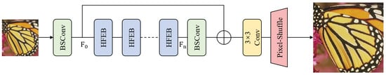
Figure 1.
The structure of the proposed RNET for lightweight image super-resolution.
Regarding the shallow feature extraction module: first, given the input low-resolution image , we use BSConv to obtain the shallow features . The structure of BSConv is shown in Figure 3. The process can be expressed as follows:
where denotes BSConv. Next, the deep feature extraction module consists of multiple directly connected Hybrid Feature Extraction Blocks (HFEBs), and this process can be expressed as:
where denotes the nth HFEB. and , respectively, denote the input features and output features of the nth HFEB. In addition, we use a BSConv layer to smooth the depth features. Lastly, the image reconstruction module consists of a standard convolution with pixel shuffling: the objective is to upsample the fused features and recover them to HR size. Finally, we fuse shallow and deep features by adding global residual connections. The process can be expressed as:
where indicates the final recovered image through the above network.
3.2. Hybrid Feature Extraction Block
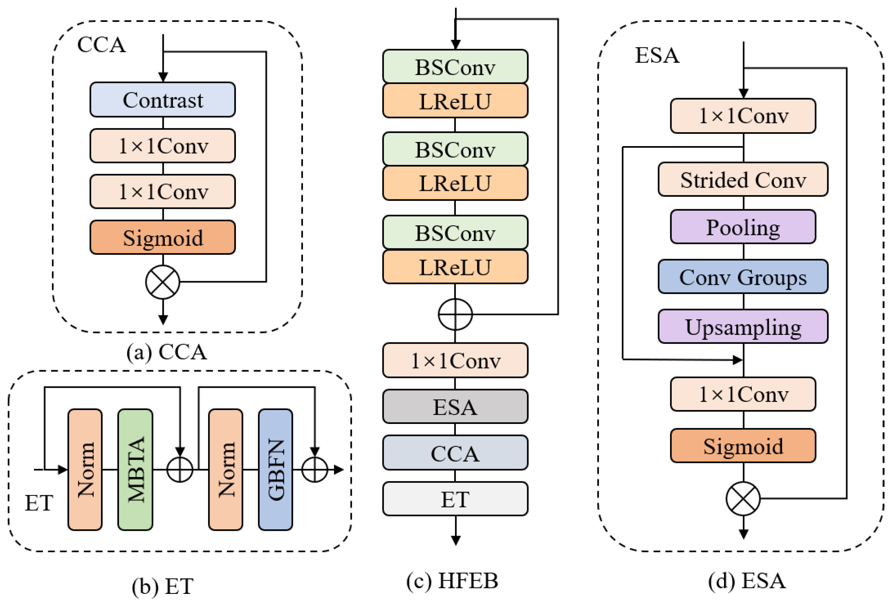
In this subsection, we introduce the Hybrid Feature Extraction Block (HFEB): the specific structure of this module is shown in Figure 2c. We use BSConv instead of traditional convolution, which greatly reduces the computational burden. Also, we use local residual connections instead of separable distillation structures. Kong et al. [19] demonstrate that the local residual structure can significantly reduce inference time while maintaining the model’s capability.
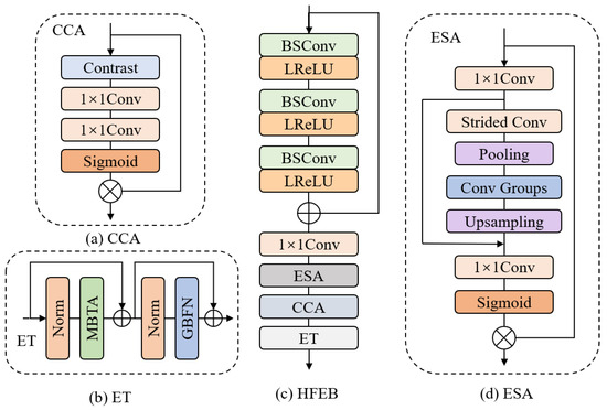
Figure 2.
(a) The architecture of CCA block. (b) The architecture of ET block (c) The architecture of our Hybrid Feature Extraction Block (HFEB). (d) The architecture of ESA block.
HFEB is divided into three main parts to extract image features: namely, a local feature extraction module, a hybrid attention mechanism, and an efficient transformer. First, we use several stacked BSConv and LeakyRelu layers to extract local features. Specifically, each BSConv layer is equipped with a LeakyRelu activation function. Given the input feature , this part can be described as:
where denotes the output of the nth BSConv and LeakyRelu combination module, denotes the LeakyRelu activation function, denotes BSConv opration, and represents the output of the entire local feature extraction module.
Next, to get more-detailed information, we first pass the output of the local feature part through a convolution before feeding it to the hybrid attention module. This module consists of a lightweight Enhanced Spatial Attention (ESA) block [16] and a Contrast-aware Channel Attention (CCA) block [22], and this process can be formulated as:
and represent the CCA block and ESA block, respectively. represents the 1 × 1 convolution. represents the output of the hybrid attention module.
Finally, to better aggregate global information, we feed the output of the hybrid attention module into the Efficient Transformer (ET) module. This module consists of Multi-BSConv head Transposed Attention (MBTA) and Gated-BSConv Feed-forward Network (GBFN); it retains the global feature extraction capability of a transformer while greatly reducing the computational burden. The whole process can be described as:
where represents the ET block. and represent the GBFN and MBTA, respectively. represents the output of the whole HFEB.
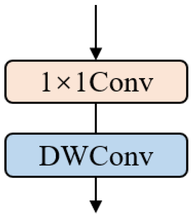
3.2.1. BSConv
BSConv is a method that decomposes the standard convolution into a point-wise convolution and a depth-wise convolution. It can be regarded as a variant of depth-separable convolution. The structure of BSConv is shown in Figure 3. Similar to depth-separable convolution, it has less computational burden than standard convolution, and it has been shown that BSConv has better results than standard convolution in most cases [20].
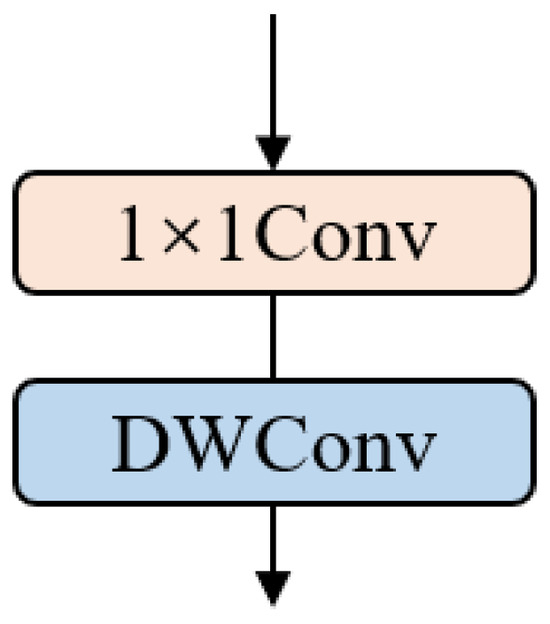
Figure 3.
The structure of BSConv, where DWConv represents the depth-wise convolution.
3.2.2. ESA and CCA
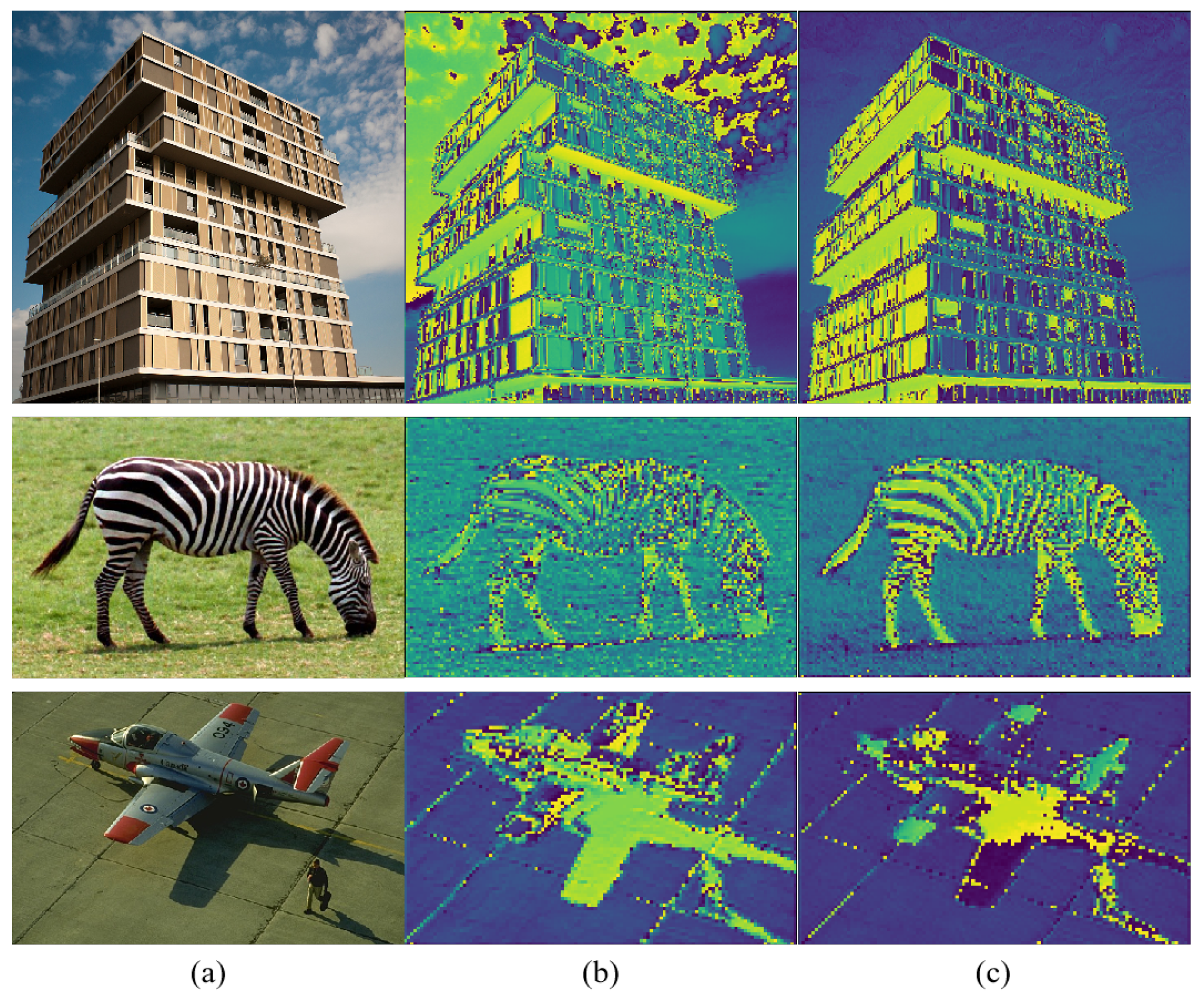
The effectiveness of ESA and CCA modules for SR tasks has been demonstrated [16,22], so we introduce these two modules into our HFEB. The structure of ESA is shown in Figure 2d. It uses a convolution to reduce the input channel, and it uses strided convolution and strided max-pooling to reduce the spatial size. Then, to obtain better results and higher efficiency, a group of BSConv layers are used to extract features instead of standard convolution. Features are processed by a convolution to restore the origin channel. Finally, a Sigmoid function generates the attention matrix and the multiplied input feature. In order to achieve both spatial and channel information, we add the CCA block [22] after the ESA block. The structure of the CCA module is shown in Figure 2a; the structure represents a channel attention module specifically designed for low-level image processing. In contrast to conventional channel attention modules, CCA adopts the sum of the standard deviation and mean instead of global pooling. This modification proves advantageous for enhancing image details and texture structure information. Figure 4 presents the visualization results of feature maps before and after the incorporation of these two modules. Upon integrating the ESA and CCA modules, the proposed HFEB in this paper demonstrates improved capability to extract clearer edge and texture information. The inclusion of these two attention modules allows our network to further enhance the accuracy of SISR.

Figure 4.
Feature map visualization results. Column (a) is the input image. Column (b) is the feature map visualization result without adding ESA and CCA modules. Column (c) is the feature map visualization result after adding ESA and CCA modules.
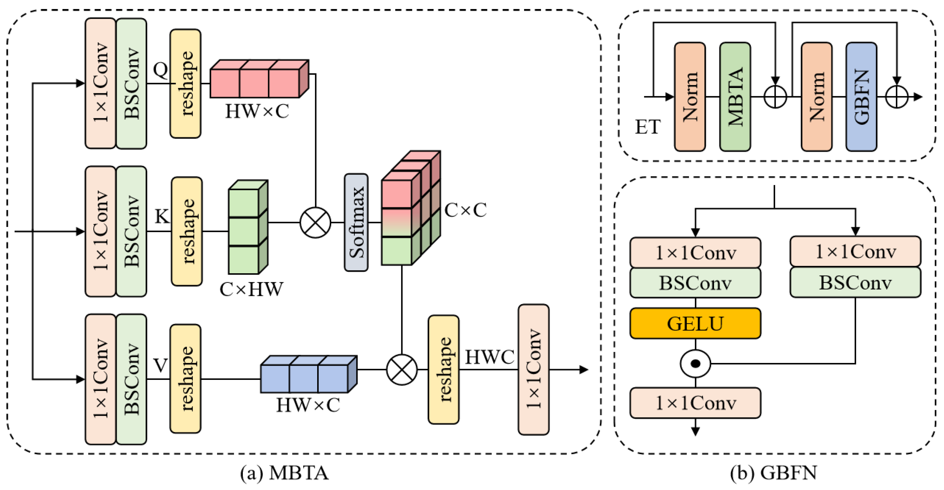
3.3. Efficient Transformer
Inspired by Restormer [41], in order to achieve better global modeling capabilities, we adopt an efficient transformer module, as shown in Figure 2b, consisting of MBTA and GBFN to further improve the performance of the network. The specific structure is shown in Figure 5.
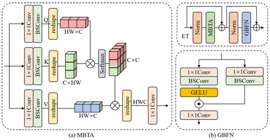
Figure 5.
The architecture of our Efficient Transformer (ET) block. (a) The architecture of MBTA in ET. (b) The architecture of GBFN in ET.
3.3.1. Multi-BSConv Head Transposed Attention (MBTA)
The computational cost in a traditional transformer mainly comes from the self-attention layer. The time and memory complexity of the key-query dot-product interaction grows quadratically with the spatial resolution of the input. MBTA, on the other hand, greatly reduces the computational overhead by using cross-channel rather than cross-space self-attention; the specific structure is shown in Figure 5a. The MBTA process is described below: for the input nominal , we first achieve cross-channel pixel-level feature aggregation by point-wise convolution, and subsequently, we use BSConv to extract channel contextual information. The advantage of using deep convolution is that it can better focus on the local context before generating the global feature map. The query (Q), key (K), and value (V) are generated from the above process. This process can be formulated as:
where denotes the BSConv, denotes the point-wise convolution, and LN denotes the layer normalization.
Next, a transposed attention map of size is generated by reshaping the query and key projection via their dot product. This process can be formulated as:
where denotes the function of softmax to generate the probability map, is a learnable scaling parameter to control the size of the dot product of K and Q before applying the softmax function, and indicates the point-wise convolution.
The above operation successfully reduces the complexity of the transformer to a linear channel complexity, effectively reducing the computational cost.
3.3.2. Gated-BSConv Feed-Forward Network (GBFN)
To further recover the structural information, the efficient transformer employs a Gated-BSConv Feed-forward Network (GBFN). This feed-forward network has two important components: a gating mechanism and BSConv. Similar to MBTA, we use BSConv to learn the local information between spatially adjacent pixels, which is very effective for learning local similarity information of images for recovery and reconstruction. The specific structure is shown in Figure 5b. This process can be formulated as follows:
where denotes the GELU function, LN denotes the layer normalization, ⊙ denotes element-wise multiplication, and denotes a point-wise convolution.
Overall, the GBFN controls the information flow through the respective hierarchical levels in our pipeline, thereby allowing each level to focus on the fine details complementary to the other levels. In contrast to the MBTA, the GBFN is able to provide richer contextual information.
3.4. Loss Function
Our network is optimized with a mean absolute error (MAE, also known as L1) loss function to facilitate a fair comparison. The loss function is described as follows: given a training set that contains several pairs of LR and HR inputs, the training objective is then to minimize the L1 loss function:
where denotes the parameter set of the network, and is the L1 norm. The loss function is optimized by using Adam optimizer.
4. Experiments
In this section, we use five benchmark datasets to evaluate the performance of our proposed method. First, we introduce the datasets used along with the evaluation metrics. Then, the superiority of the proposed method is demonstrated in terms of both visualization and evaluation metrics. Finally, the complexity and computational cost of the proposed model are explored.
4.1. Experiment Setup
4.1.1. Datasets and Metrics
We used 800 images from the DIV2K dataset [42] for training. We evaluated the performance of the different methods using five standard benchmark datasets from Set5 [43], Set14 [44], BSD100 [45], Urban100 [46], and Manga109 [47]. We evaluated the mean Peak Signal-to-Noise Ratio (PSNR) and Structural SIMilarity (SSIM) on the Y-channel. And we downscale HR images with the scaling factors (×2, ×3, and ×4) using bicubic degradation models.
4.1.2. Training Details
Our model is trained on the RGB channel, and we enhance the training data by randomly flipping the images 90°, 180°, 270°, and horizontally. The number of HFEBs is set to 8, and the channel number is set to 48. The kernel size of all depth-wise convolutions is set to 3. The patch size for each LR input is set to , and we randomly crop HR patches of size from the ground truth. The batch size is 32. For all scales of the model, the training process is divided into two stages. In the first stage, we train the model from the beginning. In the second stage, we use a two-time warm-start strategy. In each stage, we use the Adam optimizer [48] with , . the initial learning rate is set to with cosine learning rate decay. The L1 loss function is used to optimize the model for total iterations in each stage. We implement our model on a GeForce RTX 3090 GPU using PyTorch 1.9.0; the training process takes about 40 h.
4.2. Quantitative Results
4.2.1. Comparison Results
To verify the effectiveness of our RNET, we compare it with 10 advanced efficient super-resolution models: SRCNN [2], FSRCNN [18], VDSR [3], DRRN [30], LapSRN [31], LAPAR-A [19], MemNet [32], IDN [17], IMDN [22], RFDN [49], and RLFN-S [50] with scale factors of 2, 3, and 4. The quantitative performance comparison on five benchmark test sets is shown in Table 1. Compared to other advanced methods, RNET achieves the best performance for both PSNR and SSIM while reducing the parameters by 70 K compared to the second-best method RLFN-S and by 150 K parameters compared to the third-best method RFDN.

Table 1.
Quantitative comparison with other SISR models. The best and second-best performances are in red and blue, respectively.
4.2.2. Visual Results
To further demonstrate the superiority of our proposed RNET, we display the visual results compared with five advanced methods: SRCNN [2], IDN [17], IMDN [22], RFDN [49], and RLFN-S [50], as shown in Figure 6. The test results show that most methods cannot reconstruct the grid image clearly; by contrast, our RNET is able to obtain sharper results. Taking the top image in Figure 6 as an example, most methods of comparison output heavy aliasing. Earlier methods such as SRCNN [2], IDN [17], and IMDN [22] lose most of the structure due to limited network depth and feature extraction capability. Recent methods RFDN [49] and RLFN-S [50], on the other hand, are able to recover most of the outlines but not the texture details of the image. Compared with that, our method can reconstruct more details and obtain higher visual quality. This can be attributed to the global information extraction capability of the transformer.
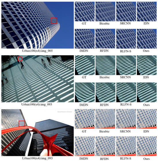
Figure 6.
Visual comparison of RNET with other methods at ×4 SR. From the figure, we can see that our method can generate more details of the image.
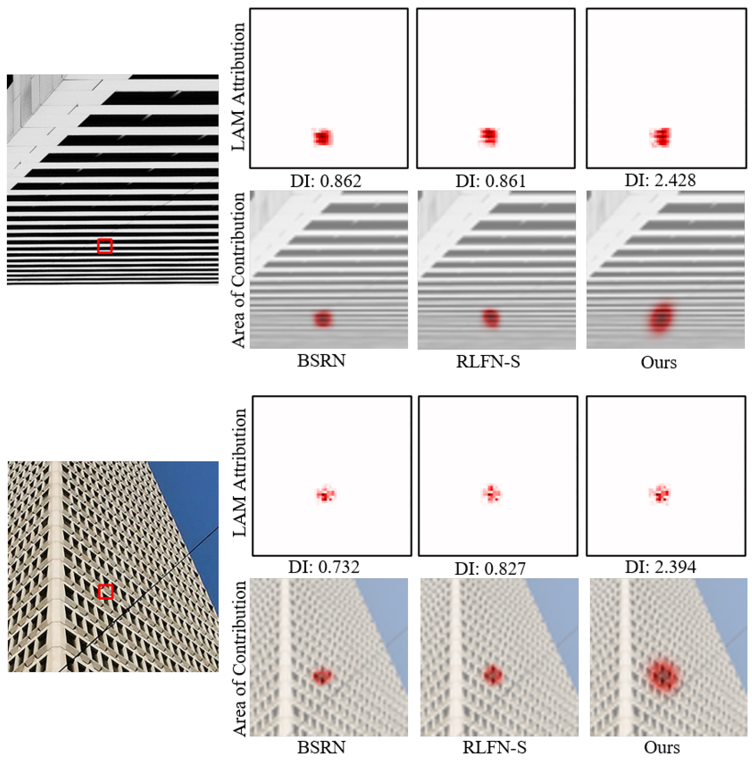
4.2.3. LAM Results
To observe the range of pixels utilized in SR reconstruction, we resort to a diagnostic tool called Local Attribution Maps (LAMs) [51], which is an attribution method specifically designed for SR. Using the LAM approach, we can identify which pixels contribute the most to the reconstruction of the selected regions. The Diffusion Index (DI) illustrates the range of relevant and utilized pixels, with a higher DI indicating a broader range of used pixels. We compare our model with BSRN [52] and RLFN-S [50], and the LAM results are shown in Figure 7. Thanks to the transformer module, RNET exhibits the widest range of pixels inferred for SR images and achieves the highest DI value. The experimental results are highly consistent with our expectations and, from an interpretability perspective, substantiate that our proposed RNET leverages the long dependencies offered by the transformer, enabling it to utilize more pixels and thus attain better performance.
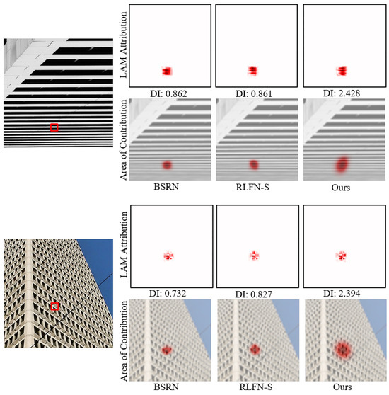
Figure 7.
LAM results of our RNET, BSRN, and RLFN-S. We can see that our RNET performs SR reconstruction based on a wider range of pixels.
4.2.4. Computational Cost and Model Complexity Analysis
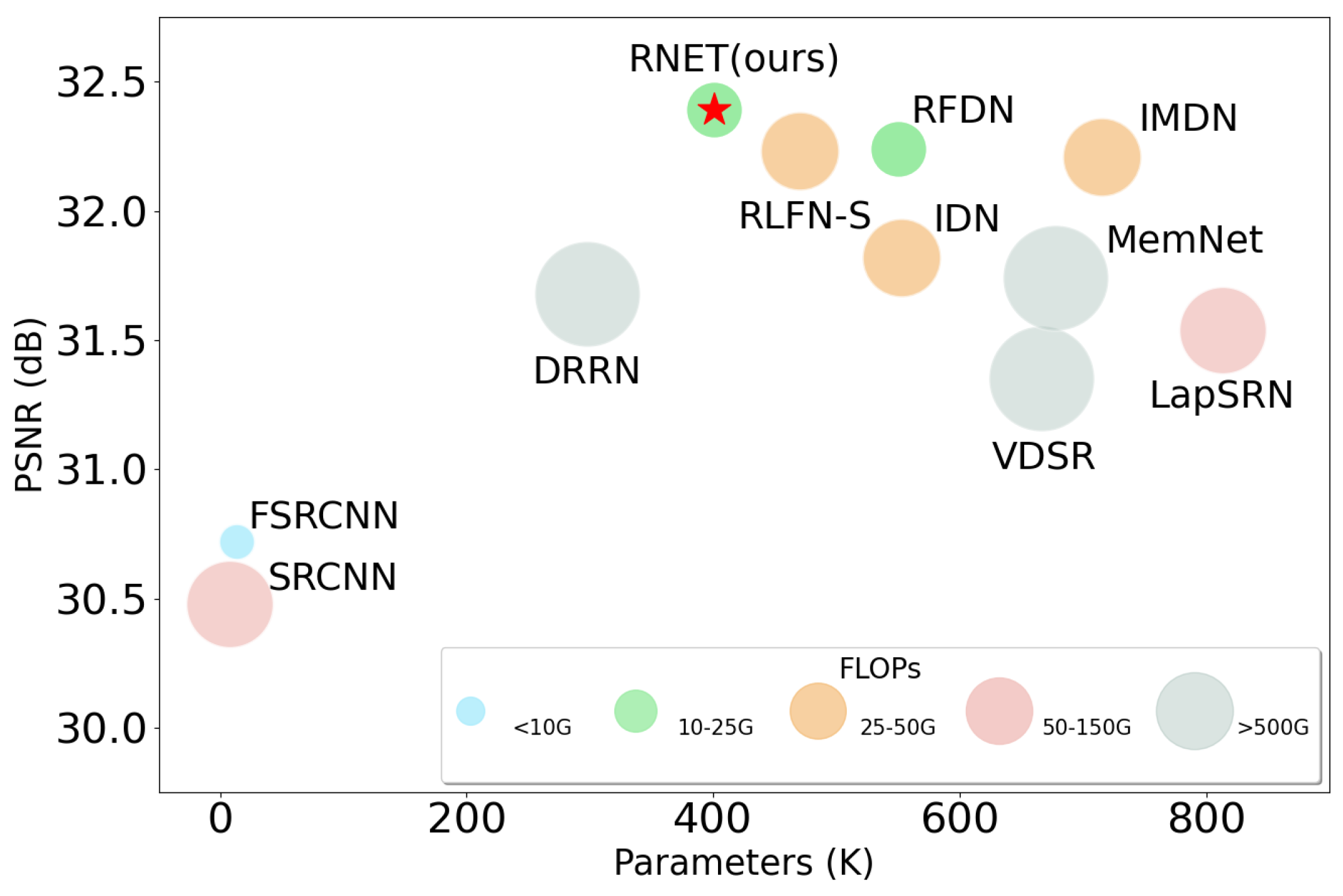
To fully investigate the efficiency of each model and demonstrate the advantages of our RNET in terms of complexity, we provide a detailed comparison of each model in Table 2, where FLOPs and Activations are the computational results when using the ×4 model with a image as input, and runtime and memory are the average results obtained by inference on the BSDS100 dataset tested 10 times using an RTX3070-8G GPU (Taipei, China). To make the results more intuitive, we also add the classical single-image super-resolution networks VDSR [3] and DRRN [30] as references. It can be seen that our proposed RNET has the second-fewest (401 K) number of parameters, the fewest (20.4 G) FLOPs, and the third-fewest Activations (0.17 G) thanks to our use of BSConv, which can efficiently extract effective features while mitigating the computation. Meanwhile, because our proposed RNET uses the transformer structure, it slightly lags behind other convolutional-neural-network-based methods in terms of inference speed and memory usage, but thanks to our use of local residual connections and the improved self-attention module, this gap is not very large and is perfectly acceptable. We visualize the trade-off between the number of parameters, FLOPs, and performance of each model in Figure 8. We can see from the figure that our RNET achieves a good balance between computational complexity and performance.
Table 2.
The results of model efficiency and computational cost.
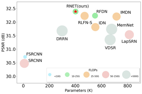
Figure 8.
A comparison of performance and model complexity on Set5 dataset; the upscale factor is ×4.
4.2.5. Comparison with Other Transformer-Based Methods
Currently, there are two mainstream approaches to solve the problem of high computation brought by vision transformers: one is to use a sliding window, also known as a swin transformer, such as SwinIR [11]; the other approach is to improve the self-attention part—for example, ESRT [53] uses the splitting factor approach to reduce the computational burden brought by the self-attention. The RNET proposed in this paper uses cross-channel self-attention to achieve the same purpose. We provide a detailed comparison of these three approaches in Table 3. It can be seen that our RNET has better performance than ESRT on the Set5 dataset and achieves similar performance to SwinIR while having the least number of parameters and FLOPs.
Table 3.
Detailed comparison with other transformer-based methods.
4.3. Ablation Study
In this subsection, we design a series of ablation experiments to analyze the effectiveness of our proposed network. We first investigate the effects of different network depths and widths on the experimental results. Then, we demonstrate the effectiveness of the ET module and explore the placement of the module. We also compare different activation functions.
4.3.1. The Depth and Width of the Network
The experimental results are shown in Table 4, where depth indicates the number of HFEBs used and width indicates the number of feature channels. From the experimental results, it can be seen that increasing both depth and width can enhance the model ability. And experiments show that network width influences results more than depth. When d increased from 6 to 8, the indicator of Urban100 increased by 0.21 db, but when d increased from 8 to 10, the indicator only increased by 0.05 db, while at the same time, the parameters increased to 479 K. And when w increased from 32 to 48, the indicator on Urban100 increased by 0.43 dB, but from 48 to 56, the indicator only showed a slight increase or even a decrease. But the parameters reach 513 K. From Table 4, when d = 10 and w = 56, the PSNR on all five benchmark test sets are improved, but the parameters of the network reach 638 K. In order to better balance the performance of the network with the parameters, we finally set the depth and width of the network to 8 and 48, respectively.
Table 4.
Ablation studies of different depths and widths of the network, where d indicates the number of HFEBs used, and w indicates the number of feature channels.
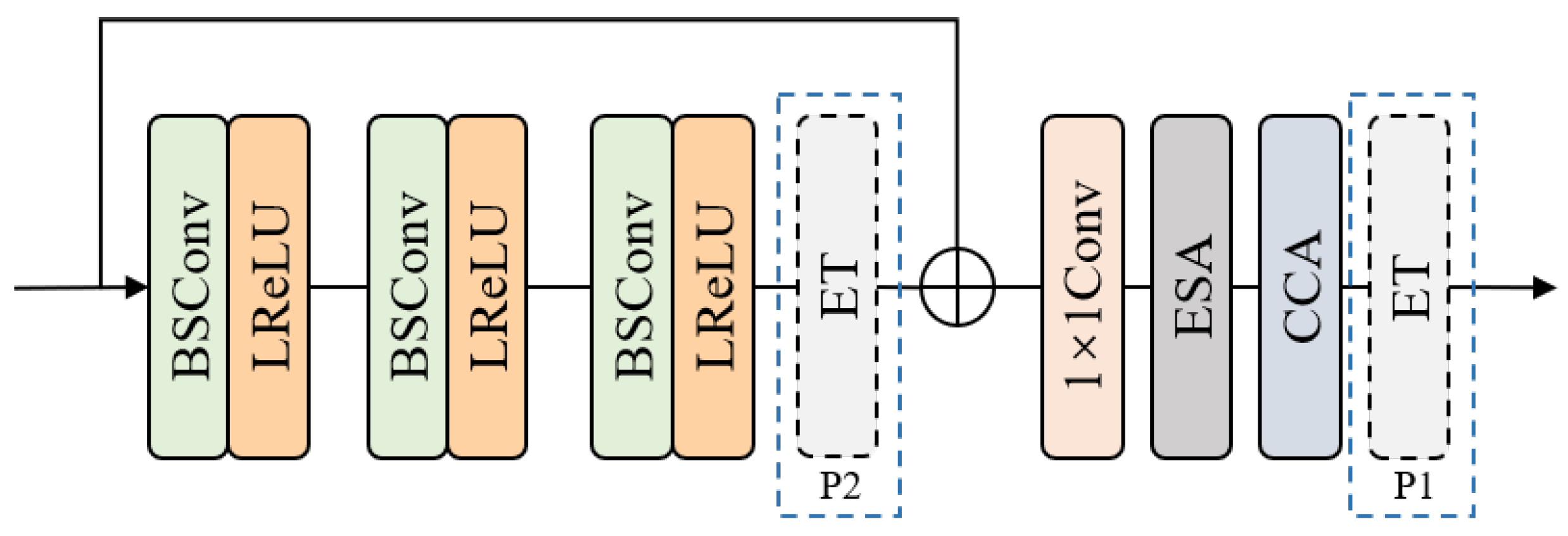
4.3.2. Ablation Study of Efficient Transformer (ET) Block
We performed ablation experiments to separately verify the impact of different convolutions in our proposed ET module and the effectiveness of the ET module. Within the two key components of the ET module, MBTA and GBFN, we replaced BSConv with traditional Depth-Wise Convolution (DWConv). The experimental results are shown in Table 5. Using BSConv in the ET module introduces an insignificant increase in parameters, but it improves the model’s performance on all five benchmark test sets. Therefore, we employed BSConv for channel feature extraction in the final ET module.
Table 5.
Quantitative comparison of the position of ET block and different convolutions used in ET.
Subsequently, to verify the effectiveness of the ET module, we placed the ET module at Position 1 (P1 in Figure 9) or Position 2 (P2 in Figure 9) or removed the ET module altogether. The experimental results are shown in Table 5. After removing the ET module, the network’s performance significantly decreased on all five benchmark datasets. When the ET module was placed at Position 2, there was a slight decline in the results on these datasets. These results demonstrate that the ET module at Position 1 can effectively enhance the capacity of the HFEB model. Consequently, in the final model, we positioned the ET module at Position 1.
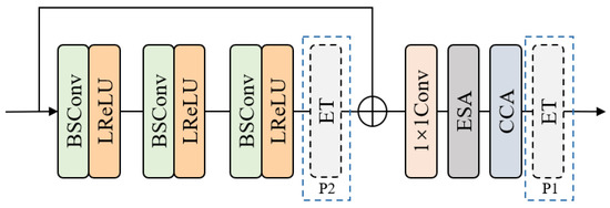
Figure 9.
The structure of HFEB and possible positions of ET in HFEB.
4.3.3. Different Activation Function in HFEB
We designed an ablation experiment to explore the effectiveness of the activation function in HFEB. The results in Table 6 show that different activation functions significantly affect the performance of the model. Among these activation functions, LeakyRelu obtains a significant performance gain, especially on the Urban100 and Manga109 datasets. Therefore, we chose LeakyReLU as the activation function in our model.
Table 6.
Ablation study using different activation functions in HFEB.
4.3.4. Effectiveness of ESA and CCA Blocks
In order to verify the effectiveness of the ESA and CCA modules, we sequentially removed these two modules from the HFEB network proposed in this paper, re-trained the ×4 scale model, then tested the network on each of the five benchmark datasets. And the experimental results are shown in Table 7. The experiments show that after removing the two attention modules, the performance of our network on all the five benchmark datasets shows some degradation. At the same time, we find that both the ESA and CCA modules hardly increase the complexity of the whole model—only increasing the number of parameters by about 2%—and result in a PSNR gain of about 0.1 db on each dataset. Thus, the ESA with CCA module used in this paper is able to give the model a performance boost at a small cost.
Table 7.
Ablation studies of the effectiveness of ESA and CCA blocks, where ✓ indicates the block is used, and ✗ indicates the block is not used.
5. Conclusions
In this paper, we propose a novel Residual Network with Efficient Transformer (RNET) for lightweight single-image super-resolution. RNET achieves a good balance between performance and model parameters. Specifically, we adopt a local residual connection structure as the backbone network for deep feature extraction modules. Compared to the widely used knowledge distillation structure, this structure significantly enhances inference speed. Concurrently, we utilize BSConv to replace traditional convolutional operations, which greatly reduces the number of required parameters. To fully exploit global information while avoiding excessive computational redundancy, we introduce an efficient transformer module that comprises channel-wise self-attention mechanisms and an efficient gated feed-forward module. Experimental results demonstrate that our method can effectively utilize a broader range of pixel information, as verified by the evaluation results from LAM. To further enhance the model’s representative capacity and accuracy, we also integrate a hybrid channel and spatial attention module. Extensive experiments show that our method achieves the best performance across five commonly used benchmark test sets. Concurrently, images reconstructed using our method exhibit the best visual results and richest details. Of particular note, RNET possesses only 400 K parameters and 20 G FLOPs: successfully achieving outstanding balance between performance and model complexity. Moreover, when processing single-image inference, RNET takes less than 30 milliseconds and occupies only 230 MB of memory. These characteristics hold significant value for promoting the practical application of single-image super-resolution techniques. In the future, we will further optimize the self-attention module to reduce memory usage. And we will expand the model so that it can be applied to more-challenging tasks, such as classical image super-resolution and real-world image super-resolution.
Author Contributions
Conceptualization, F.Y. and Z.Z.; methodology, F.Y.; software, F.Y.; validation, F.Y., S.L. and Z.Z.; formal analysis, F.Y. and S.L.; investigation, F.Y. and S.L.; resources, F.Y., Z.Z. and Y.S.; data curation, F.Y.; writing—original draft preparation, F.Y., Y.S. and Z.Z.; writing—review and editing, Z.Z. and Y.S.; visualization, F.Y. and S.L.; supervision, Y.S.; project administration, F.Y. and Z.Z. All authors have read and agreed to the published version of the manuscript.
Funding
This research received no external funding.
Institutional Review Board Statement
Not applicable.
Informed Consent Statement
Not applicable.
Data Availability Statement
Data are contained within the article.
Conflicts of Interest
The authors declare no conflicts of interest.
References
- Freeman, W.T.; Pasztor, E.C.; Carmichael, O.T. Learning low-level vision. Int. J. Comput. Vis. 2000, 40, 25–47. [Google Scholar] [CrossRef]
- Dong, C.; Loy, C.C.; He, K.; Tang, X. Image super-resolution using deep convolutional networks. IEEE Trans. Pattern Anal. Mach. Intell. 2015, 38, 295–307. [Google Scholar] [CrossRef] [PubMed]
- Kim, J.; Lee, J.K.; Lee, K.M. Accurate image super-resolution using very deep convolutional networks. In Proceedings of the IEEE Conference on Computer Vision and Pattern Recognition, Las Vegas, NV, USA, 27–30 June 2016; pp. 1646–1654. [Google Scholar]
- Zhang, Y.; Tian, Y.; Kong, Y.; Zhong, B.; Fu, Y. Residual dense network for image super-resolution. In Proceedings of the IEEE Conference on Computer Vision and Vattern Recognition, Salt Lake City, UT, USA, 18–22 June 2018; pp. 2472–2481. [Google Scholar]
- Vaswani, A.; Shazeer, N.; Parmar, N.; Uszkoreit, J.; Jones, L.; Gomez, A.N.; Kaiser, Ł.; Polosukhin, I. Attention is all you need. Adv. Neural Inf. Process. Syst. 2017, 30, 6000–6010. [Google Scholar]
- Dosovitskiy, A.; Beyer, L.; Kolesnikov, A.; Weissenborn, D.; Zhai, X.; Unterthiner, T.; Dehghani, M.; Minderer, M.; Heigold, G.; Gelly, S.; et al. An image is worth 16x16 words: Transformers for image recognition at scale. arXiv 2020, arXiv:2010.11929. [Google Scholar]
- Liu, Z.; Lin, Y.; Cao, Y.; Hu, H.; Wei, Y.; Zhang, Z.; Lin, S.; Guo, B. Swin transformer: Hierarchical vision transformer using shifted windows. In Proceedings of the IEEE/CVF International Conference on Computer Vision, Montreal, BC, Canada, 11–17 October 2021; pp. 10012–10022. [Google Scholar]
- Chen, H.; Wang, Y.; Guo, T.; Xu, C.; Deng, Y.; Liu, Z.; Ma, S.; Xu, C.; Xu, C.; Gao, W. Pre-trained image processing transformer. In Proceedings of the IEEE/CVF Conference on Computer Vision and Pattern Recognition, Nashville, TN, USA, 20–25 June 2021; pp. 12299–12310. [Google Scholar]
- Wang, Z.; Cun, X.; Bao, J.; Zhou, W.; Liu, J.; Li, H. Uformer: A general u-shaped transformer for image restoration. In Proceedings of the IEEE/CVF Conference on Computer Vision and Pattern Recognition, New Orleans, LA, USA, 18–24 June 2022; pp. 17683–17693. [Google Scholar]
- Li, W.; Lu, X.; Lu, J.; Zhang, X.; Jia, J. On efficient transformer and image pre-training for low-level vision. arXiv 2021, arXiv:2112.10175. [Google Scholar]
- Liang, J.; Cao, J.; Sun, G.; Zhang, K.; Van Gool, L.; Timofte, R. Swinir: Image restoration using swin transformer. In Proceedings of the IEEE/CVF International Conference on Computer Vision, Montreal, BC, Canada, 11–17 October 2021; pp. 1833–1844. [Google Scholar]
- Lim, B.; Son, S.; Kim, H.; Nah, S.; Mu Lee, K. Enhanced deep residual networks for single image super-resolution. In Proceedings of the IEEE Conference on Computer Vision and Pattern Recognition Workshops, Honolulu, HI, USA, 21–26 July 2017; pp. 136–144. [Google Scholar]
- Zhang, K.; Zuo, W.; Zhang, L. Learning a single convolutional super-resolution network for multiple degradations. In Proceedings of the IEEE conference on Computer Vision and Pattern Recognition, Salt Lake City, UT, USA, 18–23 June 2018; pp. 3262–3271. [Google Scholar]
- Chu, X.; Zhang, B.; Xu, R. Multi-objective reinforced evolution in mobile neural architecture search. In Proceedings of the Computer Vision—ECCV 2020 Workshops, Glasgow, UK, 23–28 August 2020; Proceedings, Part IV. Springer: Berlin/Heidelberg, Germany, 2021; pp. 99–113. [Google Scholar]
- Kim, J.; Lee, J.K.; Lee, K.M. Deeply-recursive convolutional network for image super-resolution. In Proceedings of the IEEE Conference on Computer Vision and Pattern Recognition, Las Vegas, NV, USA, 27–30 June 2016; pp. 1637–1645. [Google Scholar]
- Liu, J.; Zhang, W.; Tang, Y.; Tang, J.; Wu, G. Residual feature aggregation network for image super-resolution. In Proceedings of the IEEE/CVF Conference on Computer Vision and Pattern Recognition, Seattle, WA, USA, 13–19 June 2020; pp. 2359–2368. [Google Scholar]
- Hui, Z.; Wang, X.; Gao, X. Fast and accurate single image super-resolution via information distillation network. In Proceedings of the IEEE conference on Computer Vision and Pattern Recognition, Salt Lake City, UT, USA, 18–23 June 2018; pp. 723–731. [Google Scholar]
- Dong, C.; Loy, C.C.; Tang, X. Accelerating the super-resolution convolutional neural network. In Proceedings of the Computer Vision—ECCV 2016: 14th European Conference, Amsterdam, The Netherlands, 11–14 October 2016; Proceedings, Part II 14. Springer: Berlin/Heidelberg, Germany, 2016; pp. 391–407. [Google Scholar]
- Li, W.; Zhou, K.; Qi, L.; Jiang, N.; Lu, J.; Jia, J. Lapar: Linearly-assembled pixel-adaptive regression network for single image super-resolution and beyond. Adv. Neural Inf. Process. Syst. 2020, 33, 20343–20355. [Google Scholar]
- Haase, D.; Amthor, M. Rethinking depthwise separable convolutions: How intra-kernel correlations lead to improved mobilenets. In Proceedings of the IEEE/CVF Conference on Computer Vision and Pattern Recognition, Seattle, WA, USA, 13–19 June 2020; pp. 14600–14609. [Google Scholar]
- Howard, A.G.; Zhu, M.; Chen, B.; Kalenichenko, D.; Wang, W.; Weyand, T.; Andreetto, M.; Adam, H. Mobilenets: Efficient convolutional neural networks for mobile vision applications. arXiv 2017, arXiv:1704.04861. [Google Scholar]
- Hui, Z.; Gao, X.; Yang, Y.; Wang, X. Lightweight image super-resolution with information multi-distillation network. In Proceedings of the 27th ACM International Conference on Multimedia, Nice, France, 21–25 October 2019; pp. 2024–2032. [Google Scholar]
- Tian, C.; Xu, Y.; Zuo, W. Image denoising using deep CNN with batch renormalization. Neural Netw. 2020, 121, 461–473. [Google Scholar] [CrossRef] [PubMed]
- Pan, J.; Ren, W.; Hu, Z.; Yang, M.H. Learning to deblur images with exemplars. IEEE Trans. Pattern Anal. Mach. Intell. 2018, 41, 1412–1425. [Google Scholar] [CrossRef] [PubMed]
- Ledig, C.; Theis, L.; Huszár, F.; Caballero, J.; Cunningham, A.; Acosta, A.; Aitken, A.; Tejani, A.; Totz, J.; Wang, Z.; et al. Photo-realistic single image super-resolution using a generative adversarial network. In Proceedings of the IEEE Conference on Computer Vision and Pattern Recognition, Honolulu, HI, USA, 21–26 July 2017; pp. 4681–4690. [Google Scholar]
- Zhang, Y.; Li, K.; Li, K.; Wang, L.; Zhong, B.; Fu, Y. Image super-resolution using very deep residual channel attention networks. In Proceedings of the European Conference on Computer Vision (ECCV), Munich, Germany, 8–14 September 2018; pp. 286–301. [Google Scholar]
- Zhou, S.; Zhang, J.; Zuo, W.; Loy, C.C. Cross-scale internal graph neural network for image super-resolution. Adv. Neural Inf. Process. Syst. 2020, 33, 3499–3509. [Google Scholar]
- Wang, X.; Xie, L.; Dong, C.; Shan, Y. Real-esrgan: Training real-world blind super-resolution with pure synthetic data. In Proceedings of the IEEE/CVF International Conference on Computer Vision, Montreal, BC, Canada, 11–17 October 2021; pp. 1905–1914. [Google Scholar]
- Bashivan, P.; Rish, I.; Yeasin, M.; Codella, N. Learning representations from EEG with deep recurrent-convolutional neural networks. arXiv 2015, arXiv:1511.06448. [Google Scholar]
- Tai, Y.; Yang, J.; Liu, X. Image super-resolution via deep recursive residual network. In Proceedings of the IEEE Conference on Computer Vision and Pattern Recognition, Honolulu, HI, USA, 21–26 July 2017; pp. 3147–3155. [Google Scholar]
- Lai, W.S.; Huang, J.B.; Ahuja, N.; Yang, M.H. Deep laplacian pyramid networks for fast and accurate super-resolution. In Proceedings of the IEEE Conference on Computer Vision and Pattern Recognition, Honolulu, HI, USA, 21–26 July 2017; pp. 624–632. [Google Scholar]
- Tai, Y.; Yang, J.; Liu, X.; Xu, C. Memnet: A persistent memory network for image restoration. In Proceedings of the IEEE International Conference on Computer Vision, Venice, Italy, 22–29 October 2017; pp. 4539–4547. [Google Scholar]
- Zhang, X.; Zeng, H.; Zhang, L. Edge-oriented convolution block for real-time super resolution on mobile devices. In Proceedings of the 29th ACM International Conference on Multimedia, Virtual, 20–24 October 2021; pp. 4034–4043. [Google Scholar]
- Han, K.; Rezende, R.S.; Ham, B.; Wong, K.Y.K.; Cho, M.; Schmid, C.; Ponce, J. Scnet: Learning semantic correspondence. In Proceedings of the IEEE International Conference on Computer Vision, Venice, Italy, 22–29 October 2017; pp. 1831–1840. [Google Scholar]
- Wang, S.; Zhou, T.; Lu, Y.; Di, H. Contextual transformation network for lightweight remote-sensing image super-resolution. IEEE Trans. Geosci. Remote Sens. 2021, 60, 1–13. [Google Scholar] [CrossRef]
- Carion, N.; Massa, F.; Synnaeve, G.; Usunier, N.; Kirillov, A.; Zagoruyko, S. End-to-end object detection with transformers. In Proceedings of the Computer Vision—ECCV 2020: 16th European Conference, Glasgow, UK, 23–28 August 2020; Proceedings, Part I 16. Springer: Berlin/Heidelberg, Germany, 2020; pp. 213–229. [Google Scholar]
- Wang, W.; Xie, E.; Li, X.; Fan, D.P.; Song, K.; Liang, D.; Lu, T.; Luo, P.; Shao, L. Pyramid vision transformer: A versatile backbone for dense prediction without convolutions. In Proceedings of the IEEE/CVF International Conference on Computer Vision, Montreal, BC, Canada, 11–17 October 2021; pp. 568–578. [Google Scholar]
- Wu, H.; Xiao, B.; Codella, N.; Liu, M.; Dai, X.; Yuan, L.; Zhang, L. Cvt: Introducing convolutions to vision transformers. In Proceedings of the IEEE/CVF International Conference on Computer Vision, Montreal, BC, Canada, 11–17 October 2021; pp. 22–31. [Google Scholar]
- Xiao, T.; Singh, M.; Mintun, E.; Darrell, T.; Dollár, P.; Girshick, R. Early convolutions help transformers see better. Adv. Neural Inf. Process. Syst. 2021, 34, 30392–30400. [Google Scholar]
- Wang, S.; Zhou, T.; Lu, Y.; Di, H. Detail-preserving transformer for light field image super-resolution. In Proceedings of the AAAI Conference on Artificial Intelligence, Virtual, 22 February–1 March 2022; Volume 36, pp. 2522–2530. [Google Scholar]
- Zamir, S.W.; Arora, A.; Khan, S.; Hayat, M.; Khan, F.S.; Yang, M.H. Restormer: Efficient transformer for high-resolution image restoration. In Proceedings of the IEEE/CVF Conference on Computer Vision and Pattern Recognition, New Orleans, LA, USA, 18–24 June 2022; pp. 5728–5739. [Google Scholar]
- Agustsson, E.; Timofte, R. Ntire 2017 challenge on single image super-resolution: Dataset and study. In Proceedings of the IEEE Conference on Computer Vision and Pattern Recognition Workshops, Honolulu, HI, USA, 21–26 July 2017; pp. 126–135. [Google Scholar]
- Bevilacqua, M.; Roumy, A.; Guillemot, C.; Alberi-Morel, M.L. Low-Complexity Single-Image Super-Resolution Based on Nonnegative Neighbor Embedding. In Proceedings of the British Machine Vision Conference, Surrey, UK, 3–7 September 2012; pp. 1–10. Available online: https://people.rennes.inria.fr/Aline.Roumy//publi/12bmvc_Bevilacqua_lowComplexitySR.pdf (accessed on 26 December 2023).
- Zeyde, R.; Elad, M.; Protter, M. On single image scale-up using sparse-representations. In Proceedings of the Curves and Surfaces: 7th International Conference, Avignon, France, 24–30 June 2010; Revised Selected Papers 7. Springer: Berlin/Heidelberg, Germany, 2012; pp. 711–730. [Google Scholar]
- Martin, D.; Fowlkes, C.; Tal, D.; Malik, J. A database of human segmented natural images and its application to evaluating segmentation algorithms and measuring ecological statistics. In Proceedings of the Proceedings Eighth IEEE International Conference on Computer Vision, ICCV, Vancouver, BC, Canada, 7–14 July 2001; Volume 2, pp. 416–423. [Google Scholar]
- Huang, J.B.; Singh, A.; Ahuja, N. Single image super-resolution from transformed self-exemplars. In Proceedings of the IEEE Conference on Computer Vision and Pattern Recognition, Boston, MA, USA, 7–12 June 2015; pp. 5197–5206. [Google Scholar]
- Matsui, Y.; Ito, K.; Aramaki, Y.; Fujimoto, A.; Ogawa, T.; Yamasaki, T.; Aizawa, K. Sketch-based manga retrieval using manga109 dataset. Multimed. Tools Appl. 2017, 76, 21811–21838. [Google Scholar] [CrossRef]
- Kingma, D.P.; Ba, J. Adam: A method for stochastic optimization. arXiv 2014, arXiv:1412.6980. [Google Scholar]
- Liu, J.; Tang, J.; Wu, G. Residual feature distillation network for lightweight image super-resolution. In Proceedings of the Computer Vision—ECCV 2020 Workshops, Glasgow, UK, 23–28 August 2020; Proceedings, Part III 16. Springer: Berlin/Heidelberg, Germany, 2020; pp. 41–55. [Google Scholar]
- Kong, F.; Li, M.; Liu, S.; Liu, D.; He, J.; Bai, Y.; Chen, F.; Fu, L. Residual local feature network for efficient super-resolution. In Proceedings of the IEEE/CVF Conference on Computer Vision and Pattern Recognition, New Orleans, LA, USA, 18–24 June 2022; pp. 766–776. [Google Scholar]
- Gu, J.; Dong, C. Interpreting super-resolution networks with local attribution maps. In Proceedings of the IEEE/CVF Conference on Computer Vision and Pattern Recognition, Nashville, TN, USA, 20–25 June 2021; pp. 9199–9208. [Google Scholar]
- Li, Z.; Liu, Y.; Chen, X.; Cai, H.; Gu, J.; Qiao, Y.; Dong, C. Blueprint separable residual network for efficient image super-resolution. In Proceedings of the IEEE/CVF Conference on Computer Vision and Pattern Recognition, New Orleans, LA, USA, 18–24 June 2022; pp. 833–843. [Google Scholar]
- Lu, Z.; Li, J.; Liu, H.; Huang, C.; Zhang, L.; Zeng, T. Transformer for single image super-resolution. In Proceedings of the IEEE/CVF Conference on Computer Vision and Pattern Recognition, New Orleans, LA, USA, 18–24 June 2022; pp. 457–466. [Google Scholar]


Disclaimer/Publisher’s Note: The statements, opinions and data contained in all publications are solely those of the individual author(s) and contributor(s) and not of MDPI and/or the editor(s). MDPI and/or the editor(s) disclaim responsibility for any injury to people or property resulting from any ideas, methods, instructions or products referred to in the content. |
© 2024 by the authors. Licensee MDPI, Basel, Switzerland. This article is an open access article distributed under the terms and conditions of the Creative Commons Attribution (CC BY) license (https://creativecommons.org/licenses/by/4.0/).