3D Phased Array Enabling Extended Field of View in Mobile Satcom Applications

Abstract

Satellite communication (satcom) is experiencing increased interest to cover the connectivity gaps of terrestrial networks. To ensure high performance and throughput for the user—and even more so in Communications-On-The-Move(COTM) systems, e.g., in aeronautics—steerable antennas such as phased arrays are required to adjust the beam so as to follow the satellite’s trajectory. The mutual movement of terminals and satellite in COTM systems calls for a broad Field of View (FoV) and, hence, poses a challenge to common planar systems. For improving the FoV, common solutions require ad hoc designs, such as multi-mode antennas, wide half-power-beamwidth antennas or metasurfaces. By contrast, 3D arrays are able to cover a wider angular region by the 3D allocation of the antennas. In this paper, the benefits and drawbacks of moving from 2D (planar) arrays to 3D phased arrays are investigated. Multiple geometrical configurations are analyzed, keeping in mind the size requirements of aeronautic terminals. The best configuration is, hence, an array capable of enhancing the FoV of the terminal. The proposed antenna architecture offers a good trade-off between design complexity and performance, and it could be further developed to become an aeronautic-grade terminal aperture.

1. Introduction

In recent years, satellite communication (satcom) has been emerging as a key technology for bridging the digital divide. Satellites orbiting in space are used to bring connectivity to rural areas and where the terrestrial network is missing.

While major effort has been undertaken on the space side and commercial constellations are already present, on the user side, the ground terminal still appears to be a bottleneck due to the difficulty in meeting hard requirements while having to retain low Size-Weight-Power-Cost (SWaP-C). In order to provide a high performance service to the user, with capabilities comparable to the terrestrial 5G network, high directivity antennas are required. However, the choice of orbit has an impact on the achievable performance: in the case of a GEosynchronous Orbit (GEO), the satellite does not move with respect to the Earth user, and the antenna only needs to be steered when in motion. On the other hand, in Low Earth Orbit (LEO), which offers relatively low latency compared to GEO, the satellite moves at a speed that depends on its altitude; therefore, the user terminal must steer to follow the satellite’s trajectory. In mobility applications, this becomes even more critical, as the antenna is placed on a moving platform (e.g., airplane, car, train, etc.). Especially for in-flight connectivity applications, a large FoV is needed to support GEO satellites above the equator when the flight route is close to the poles.

When dealing with antennas in mobility, the terminal is usually subjected to high scan angles with performance degradation beyond $\pm {60}^{°}$ [1]. Phased array antennas are a suitable candidate for beam-shaping and beam-steering capabilities that avoid mechanical components. However, planar phased arrays have a FoV that is limited by scan losses, which are mainly dictated by the cosine radiation of conventional patch radiators.

Regarding State of the Art (SoA), different solutions for enhancing the scan range of the phased array are intensively investigated. The different solutions are based on improving the Half-Power BeamWidth (HPBW) of the array element [2,3,4,5] aiming to mitigate the decadence in the scan range due to the element pattern. These solutions can extend the FoV both in elevation and azimuth but they require ad hoc and complex design. In addition to that, multi-mode/reconfigurable antennas [6,7,8,9] make use of elements that can be reconfigured to generate different radiation beams. The phenomenon is exploited, changing the radiation beam depending on the steering angle. The FoV is then subdivided into multiple subspaces, each one assigned to a specific beam. However, these solutions result in complicated ad hoc solutions for which the feeding network has to deal with multiple input/output for selecting the right mode. In addition, planar steering is not always supported, depending on the number of radiation beams the antenna is able to generate and their distribution in space.

A further category of solutions includes metasurfaces such as the High-Impedance Periodic Structure (HIPS) [10,11], Wide Angle Impedance Matching (WAIM) [12,13,14] solutions and dielectric domes, such as radome [15,16,17]. These solutions require the design of additional layers which often adds complexity to in-package solutions.

On the other hand, conformal arrays are an efficient solution for coverage extension [18,19,20,21,22,23,24], but they cannot be manufactured through planar PCBs, resulting in complicated and expensive dedicated manufacturing. By faceting the conformal array [25,26,27,28], the array can be easily manufactured through planar PCBs faces. As result, complexity in design and manufacturing can be easily reduced by keeping the performance acceptable.

In this paper, the authors present an analysis of the advantages and disadvantages of different non-planar faceted architectures in the framework of satcom Communications–On–The–Move (COTM) applications. A 3D phased array architecture is presented for mitigating FoV limitation in planar phased arrays for COTM terminals. The paper extends the work conducted in [29] by presenting an analysis of the cost and efficiency of different linear faceted arrays. Minimizing the number of facets with the minimization of performance degradation, the best linear candidate is extended to the 3D case.

The paper is organized as follows: the scenario is addressed in Section 2, the mathematical formulation in Section 3 and the numerical results in Section 4. Finally, conclusions are drawn in Section 5.

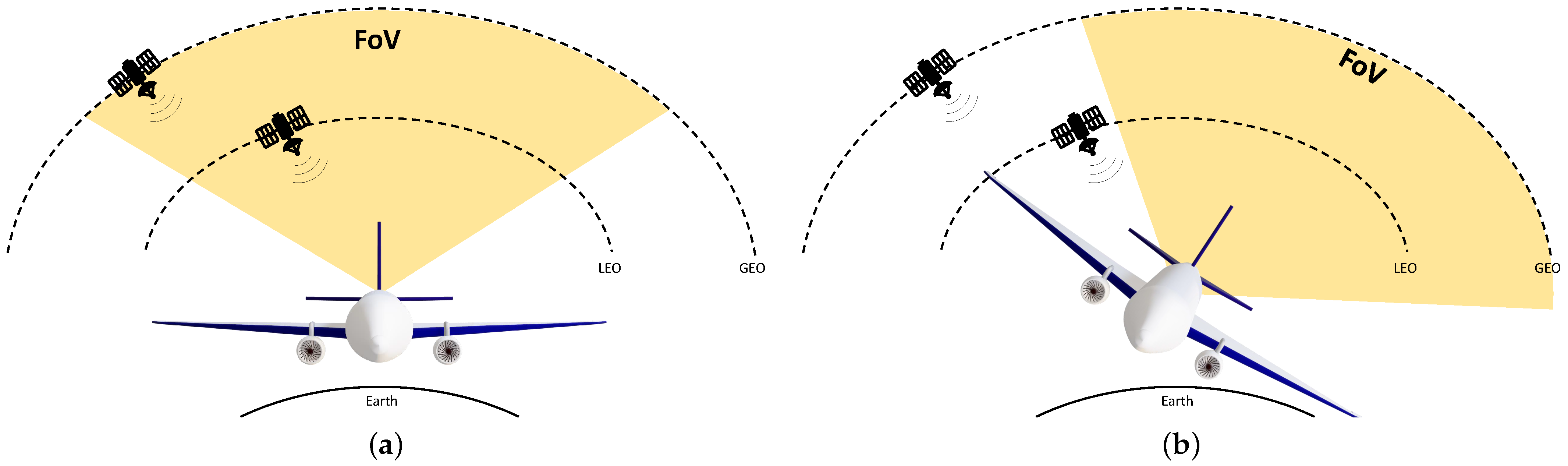
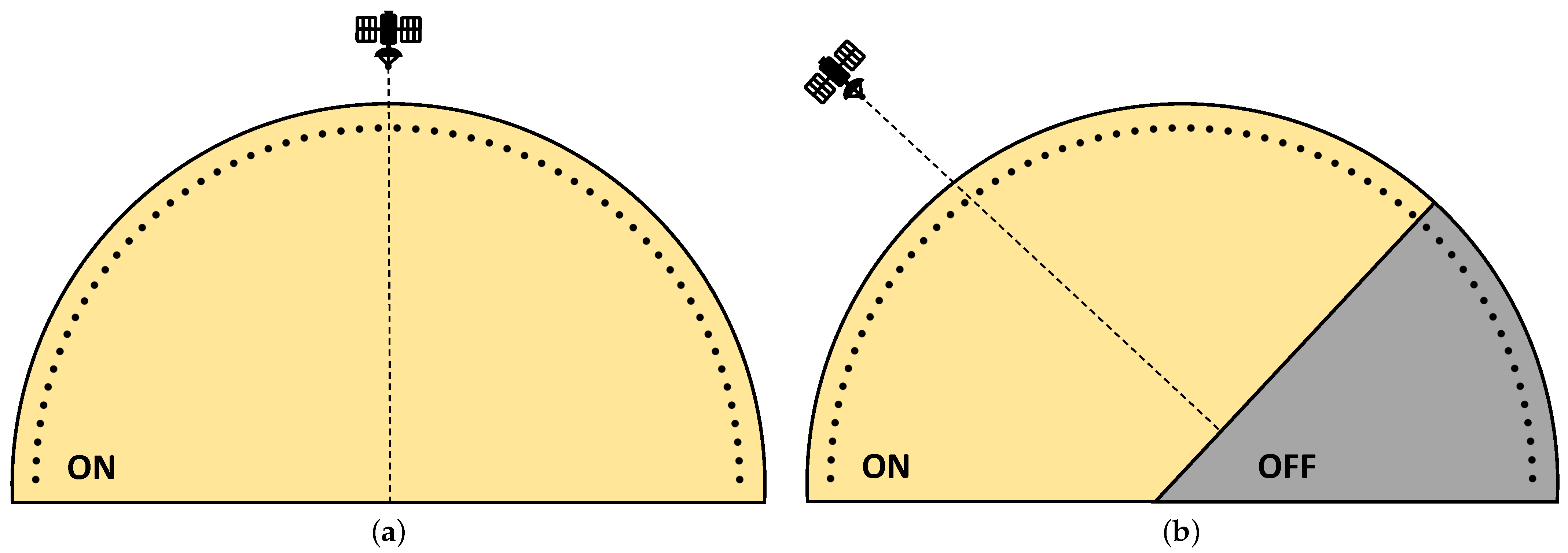
2. Scenario and Requirements: Communications on The Move (COTM)

In the following, a COTM scenario is described. In Figure 1, an example depicting in-flight connectivity scenario is shown, with an antenna mounted on an aircraft fuselage. When dealing with COTM applications, the antenna is subjected to high scan angles. In the case of aircraft applications, when the flight route is close to the poles and GEO is used, high steering angles are needed for ensuring a stable connectivity with the satellite above the equator. However, usually the performance drops when the steering is outside the range of $\pm {60}^{°}$ [1].

With respect to the sketch in Figure 1, in (a), the antenna is able to catch signals from LEO and GEO satellites. However, during the aircraft’s turn, both satellites disappear from the antenna’s FoV. In the case of LEO, a handover to another satellite in the FoV is required, while GEO remains outside the FoV.

Usually, the antenna’s FoV refers to the range of angles within which the carrier-to-noise-ratio $C/N$ allows for a reliable and robust communication [30]. In this work, the FoV is computed by considering a scan loss of 3 dB and an axial ratio of <3 dB (with a tolerance of $0.5$ dB). The choice to include the axial ratio in the FoV calculation is motivated by the prevalent use of circular polarization in satcom. When the axial ratio exceeds the set threshold, both the circular polarized component and the overall $C/N$ suffer degradation. Additionally, selecting a directivity scan loss of 3 dB outperforms the conventional ideal $cos\theta$ roll-off, ensuring satisfactory $C/N$ values overall.

In the following, the definition of requirements and the reference planar array architecture are first presented.

The requirements for the array are listed in

Table 1. Summary of the main requirements.

Figure of Merit	Value
Directivity, $D{\left(\theta ,\phi \right)}_{max}$	≈40 dBiC
Axial Ratio, $AR{\left(\theta ,\phi \right)}_{max}$	<3 dB (tolerance $0.5$ dB)
Scan Range	>$\pm {70}^{°}$
Maximum Directivity Scan Loss	3 dB

. A directivity of 40 dBiC is desirable, with a scan range of $\pm {70}^{°}$. As previously stated, the FoV is computed considering a maximum directivity scan loss of 3 dB, which outperforms the traditional $cos\theta$ gain roll-off. Moreover, an axial ratio of <3 dB is also required, with a tolerance of $0.5$ dB.

A planar array composed of $60\times 60$ elements spaced at $\lambda /2$ is considered as reference, achieving a directivity of $42.3$ dBiC. It is presented in Section 4. To enhance the FoV of the reference planar phased array architecture, 3D geometries are explored and simplified by faceting the conformal architecture. Indeed, given a 3D surface, its total surface area $\mathcal{S}$ can be expressed as $\mathcal{S}={\sum }_{n=1}^{N_f}{\mathcal{F}}_n$, where $\mathcal{F}$ denotes the discretization of the surface via facets and $N_f$ denotes the total number of facets. In an ideal hemisphere, $N_f\to \infty$ and ${\mathcal{F}}_{n=1,\dots ,N_f}\to 0$. To find a suitable 3D architecture that can be easily manufactured, a trade-off analysis is conducted, minimizing the number of facets $N_f$. This way, the 3D architecture can be easily manufactured using planar PCBs (the facets).

In the next Section, directivity and axial ratio are considered to estimate the total FoV, and their computation for different 3D array geometries is explained.

3. Mathematical Formulation

In the following, the mathematical formulation is provided to the reader. For computing the directivity and axial ratio of the 3D array, a flowchart of the methodology is depicted in Figure 2. In the following, the different blocks listed here are presented:

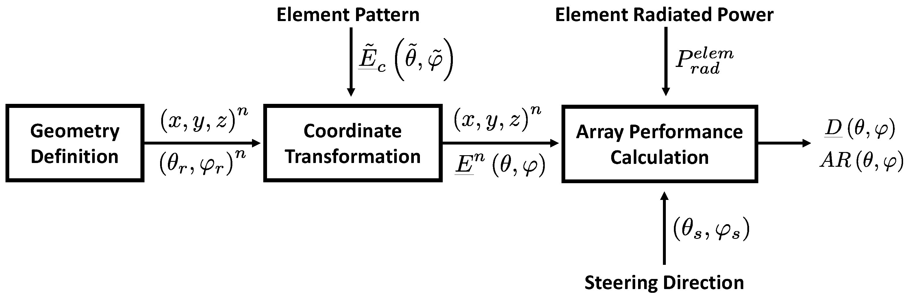
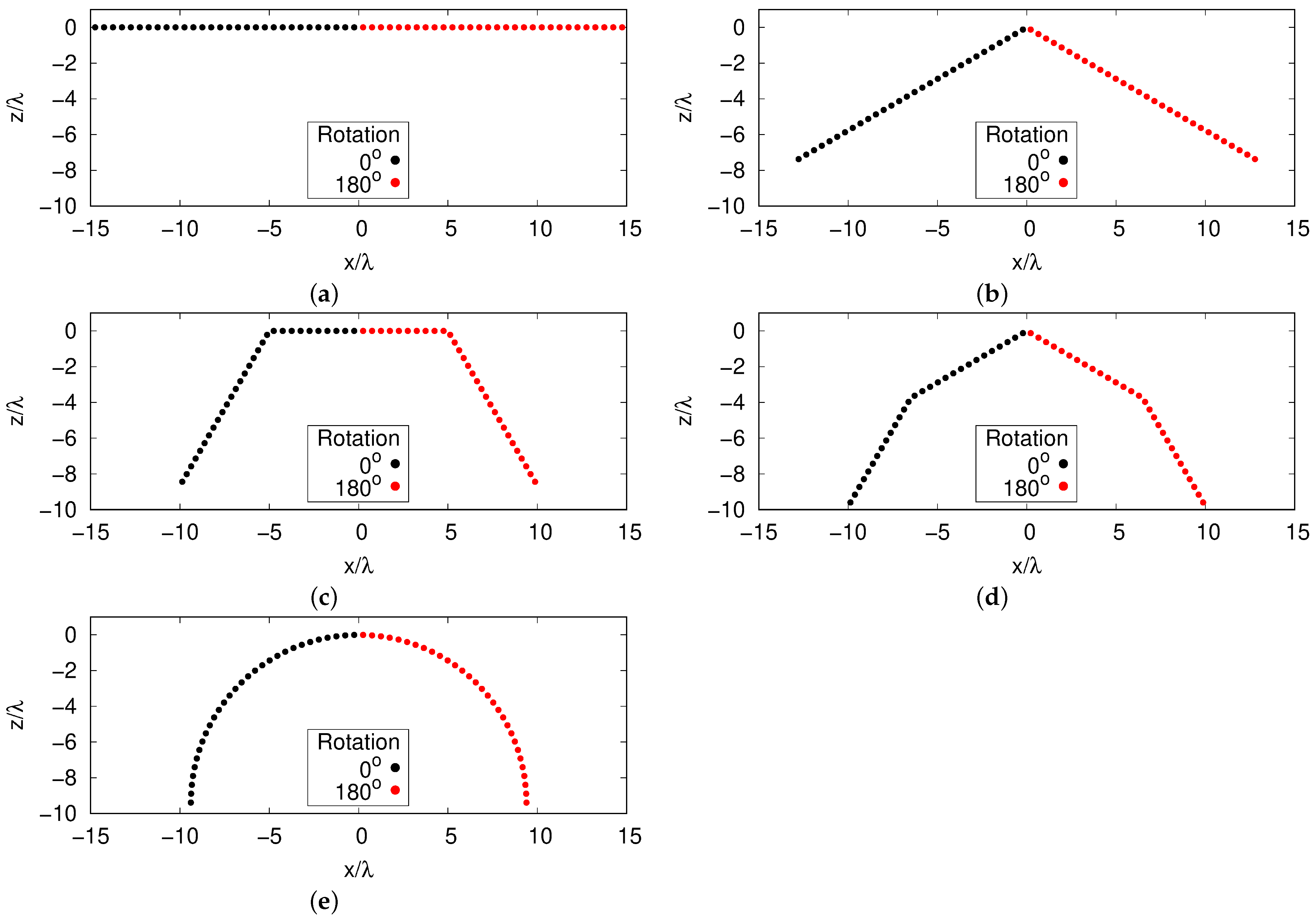
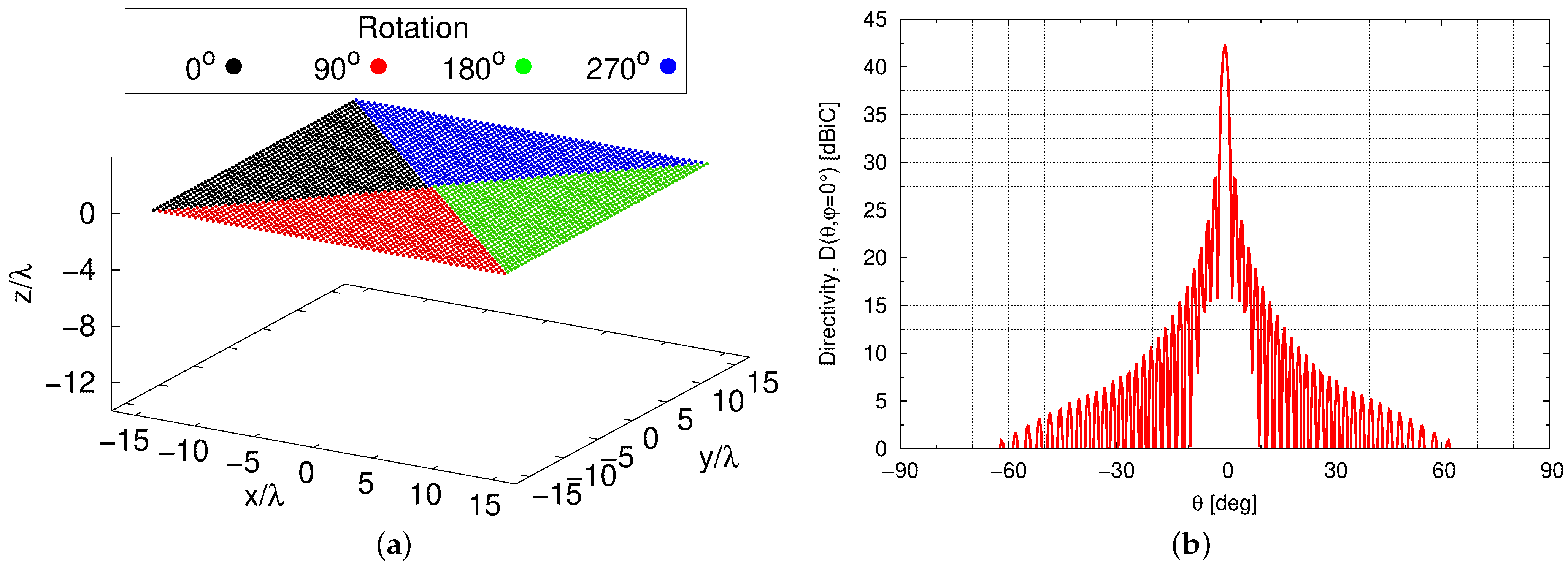
• Geometry Definition: A specific 3D geometry is first created by defining the ${\left(x,y,z\right)}^n$ positions for each antenna element. Moreover, rotation angles ${\left({\theta }_r,{\phi }_r\right)}^n$ are computed for each element.
• Coordinate Transformation: The element pattern ${\underline{\tilde{E}}}_c\left(\tilde{\theta },\tilde{\phi }\right)$ computed through full-wave simulation is rotated for each element according to the rotation angles and positions computed in the previous step.
• Array Performance Calculation: Directivity and axial ratio for the array at specific steering angle $\left({\theta }_s,{\phi }_s\right)$ are computed.

3.1. Geometry Definition

Given a specific 3D array aperture, the first step is to calculate positions ${(x,y,z)}^n$ where $n=1,\dots ,N$ represents the element index and N is the number of elements in the aperture. Additionally, since we are not dealing with isotropic sources, the element pattern must be rotated according to its position. To achieve this, rotation angles ${\left({\theta }_r,{\phi }_r\right)}^n$, respectively, in elevation and azimuth, are defined. A sketch of the coordinate system is represented in Figure 3.

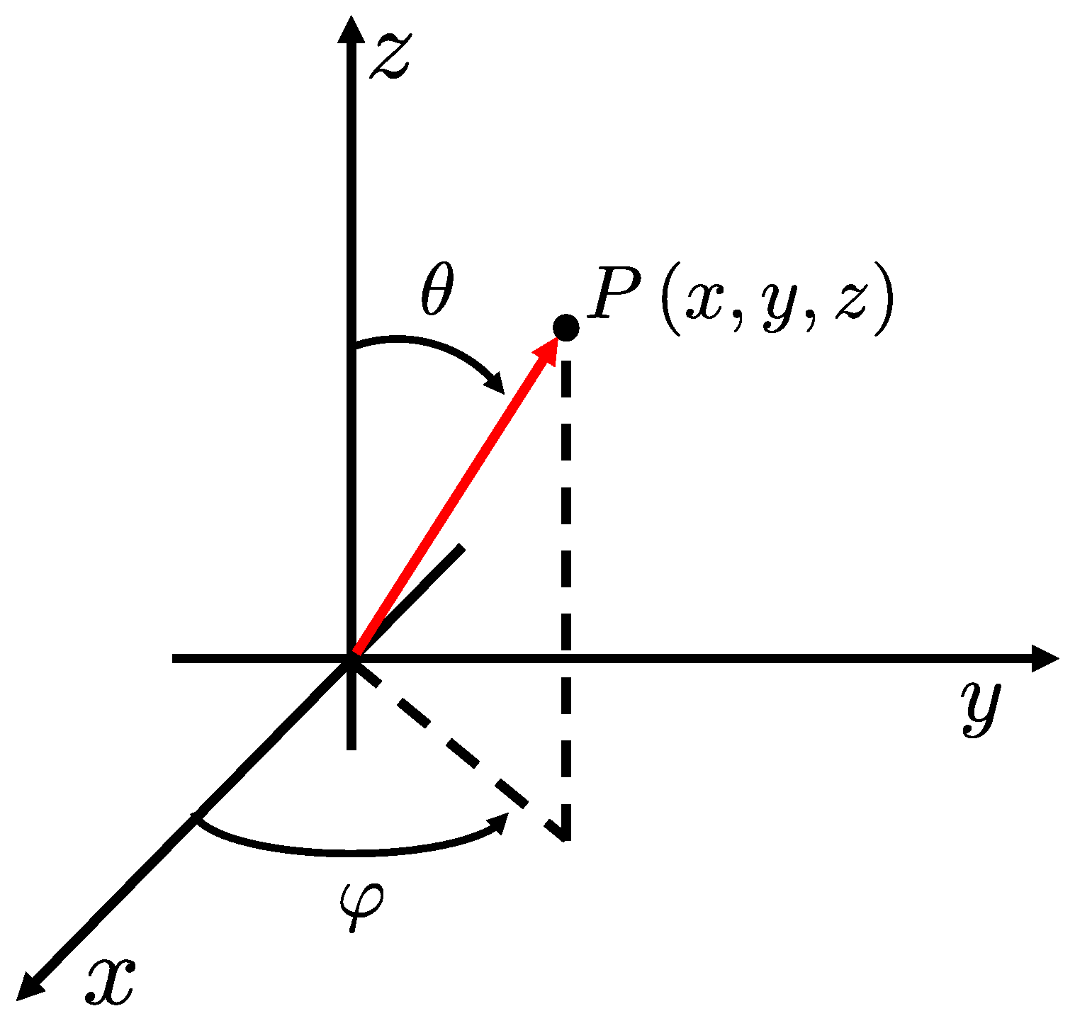
3.2. Coordinate Transformation

As previously mentioned, when dealing with non-isotropic and asymmetrical radiation sources, the stand-alone element pattern ${\underline{\tilde{E}}}_c\left(\tilde{\theta },\tilde{\phi }\right)=\left\{{\tilde{E}}_x,{\tilde{E}}_y,{\tilde{E}}_z\right\}\in \mathbb{C}$ must be rotated according to its position under the rotation angles ${\left({\theta }_r,{\phi }_r\right)}^n$. The complex far-field element pattern ${\underline{\tilde{E}}}_c\left(\tilde{\theta },\tilde{\phi }\right)$ is computed through a full-wave analysis in Ansys Electronics Desktop HFSS 2022. For this analysis, a patch antenna radiator working in receive mode in the Ka-band is designed and simulated. Element pattern and rotation formulation are presented next.

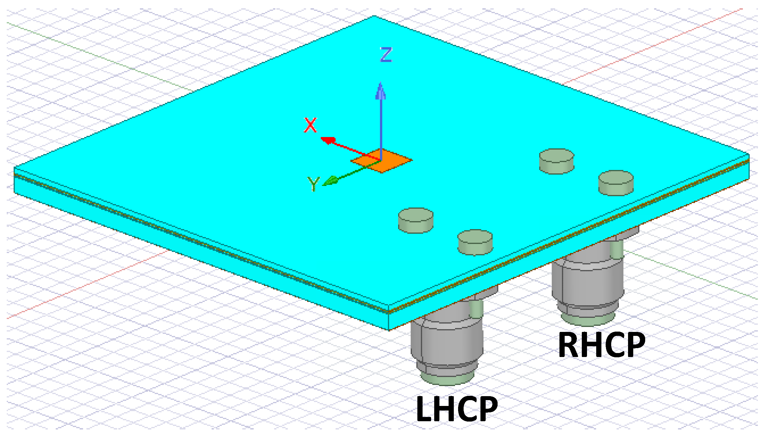
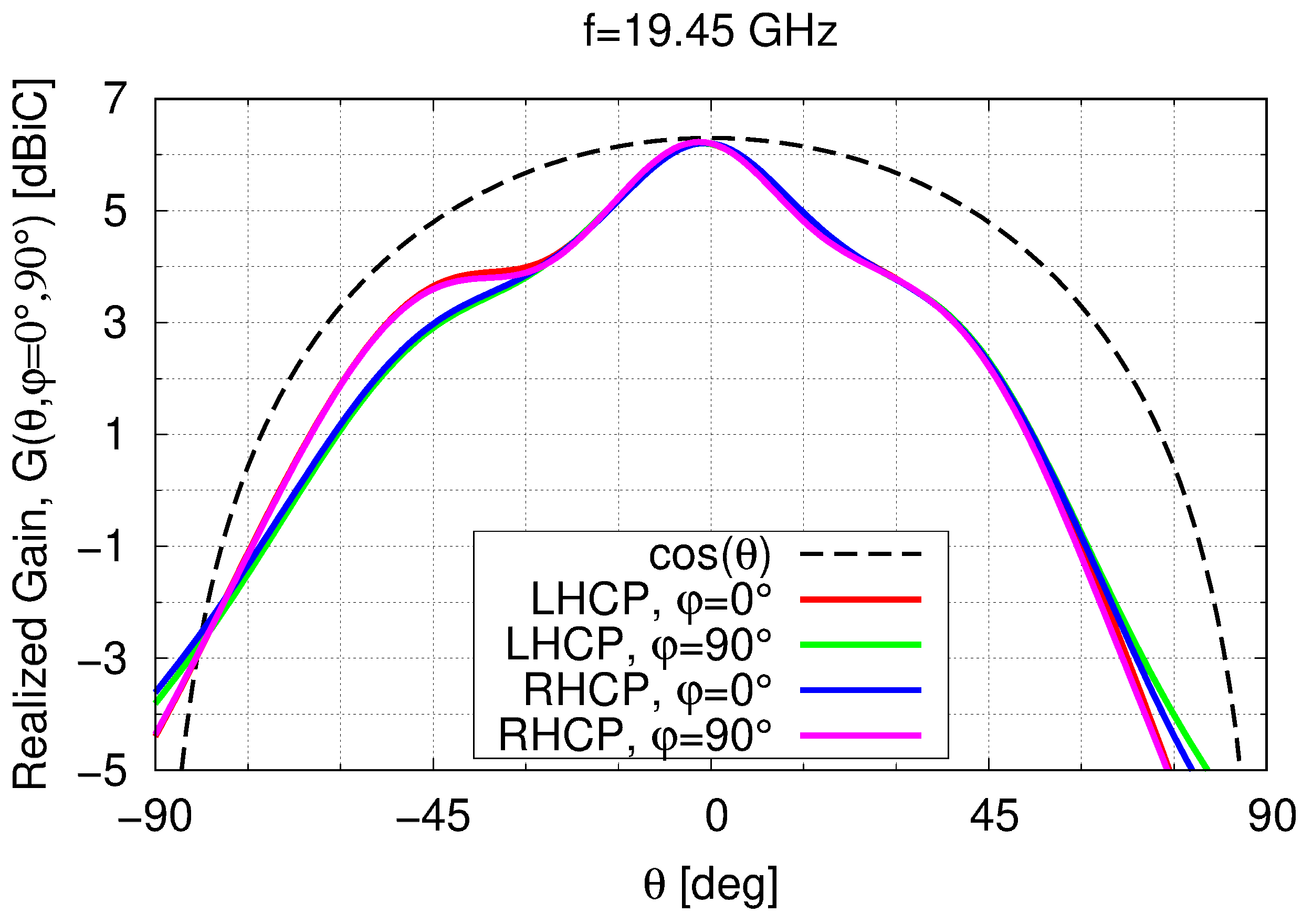
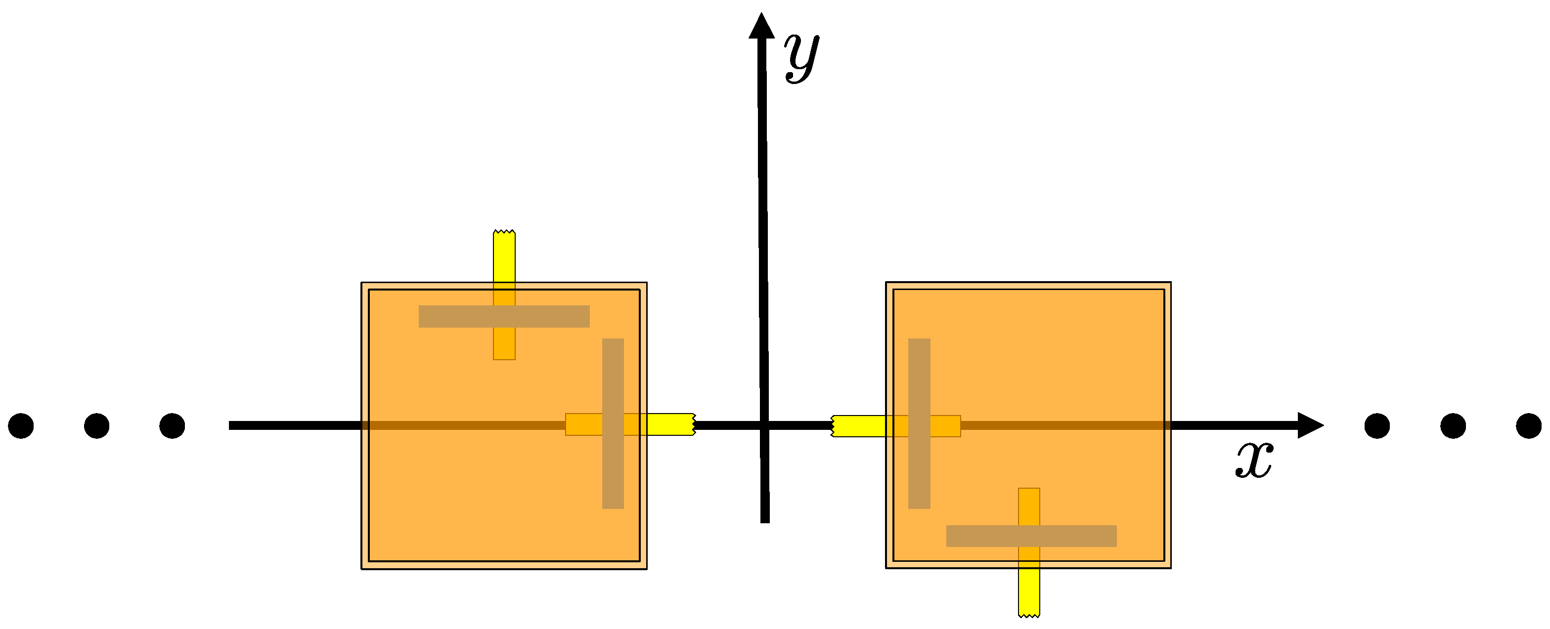
3.2.1. Single Element

An antenna designed for Ka-band satcom applications is presented [31] and is used as reference in the next. As an example, the receiver band (17.7–20.2 GHz) [32] is chosen. It is worth mentioning that this single element does not represent the final antenna solution but acts as a quasi-real scenario (e.g., realistic simulated pattern). This scenario accounts for the non-ideal hemispherical radiation of common patch radiators. Other types of antennas may be investigated, particularly solutions integrating the TX and RX parts. Additionally, mutual coupling and the integration of the antenna into an array are not considered in this work.

The HFSS model of the patch antenna is shown in Figure 4. The antenna has 2 connectors to stimulate double circular polarization, left-hand and right-hand (LHCP, RHCP), which is typical in satellite communications. The respective far field used for array calculations is depicted in Figure 5 for both polarizations. In the numerical results, only one CP polarization is considered for the sake of brevity, as both polarizations radiate a similar far field.

Indeed, it is worth mentioning that the patch exhibits asymmetrical radiation, deviating from the ideal hemispherical/isotropic radiation and its maximum value is $6.2$ dBiC. When compared with an ideal cosine distribution, the quasi-real radiation diverges significantly. To compensate for the asymmetrical radiation, the element is rotated by ${180}^{°}$ to ensure symmetrical steering along both axes. For rotation and array far-field computation, cartesian electric field ${\underline{\tilde{E}}}_c\left(\tilde{\theta },\tilde{\phi }\right)=\left\{{\tilde{E}}_x,{\tilde{E}}_y,{\tilde{E}}_z\right\}$ is exported by HFSS. In this scenario, ${\underline{\tilde{E}}}_c\left(\tilde{\theta },\tilde{\phi }\right)$ corresponds to the non-rotated field (e.g., the antenna is looking at zenith), where $\left(\tilde{\theta },\tilde{\phi }\right)$ are the spherical coordinates in the non-rotated coordinate system. It is worth emphasizing that the electric field has no information on impedance mismatch and radiation efficiency. These losses are omitted in consideration of the fact that normalized directivity is used as Figure of Merit (FoM) for FoV calculation.

3.2.2. Rotation

Considering ${\underline{\tilde{E}}}_c^{n=1,\dots ,N}\left(\tilde{\theta },\tilde{\phi }\right)={\underline{\tilde{E}}}_c\left(\tilde{\theta },\tilde{\phi }\right)$ the same for all the elements (e.g., mutual coupling is not considered), the element pattern is first sampled in cartesian coordinates as

$$\begin{array}{cc}\hfill & \tilde{x}=sin\tilde{\theta }cos\tilde{\phi }\hfill \end{array}$$

(1)

$$\begin{array}{cc}\hfill & \tilde{y}=sin\tilde{\theta }sin\tilde{\phi }\hfill \end{array}$$

(2)

$$\begin{array}{cc}\hfill & \tilde{z}=cos\tilde{\theta }.\hfill \end{array}$$

(3)

The rotated far field is then computed for each antenna position as [33]

$${\underline{E}}_c^n\left(x,y,z\right)=\left[\begin{array}{ccc}cos{\theta }_r^{n}cos{\phi }_r^n& -sin{\phi }_r^n& sin{\theta }_r^{n}cos{\phi }_r^n\\ cos{\theta }_r^{n}sin{\phi }_r^n& cos{\phi }_r^n& sin{\theta }_r^{n}sin{\phi }_r^n\\ -sin{\theta }_r^n& 0& cos{\theta }_r^n\end{array}\right]\left[\begin{array}{c}{\tilde{E}}_x\left(\tilde{x},\tilde{y},\tilde{z}\right)\\ {\tilde{E}}_y\left(\tilde{x},\tilde{y},\tilde{z}\right)\\ {\tilde{E}}_z\left(\tilde{x},\tilde{y},\tilde{z}\right)\end{array}\right]$$

(4)

and

$$\left(x,y,z\right)=\left[\begin{array}{ccc}cos{\theta }_r^{n}cos{\phi }_r^n& -sin{\phi }_r^n& sin{\theta }_r^{n}cos{\phi }_r^n\\ cos{\theta }_r^{n}sin{\phi }_r^n& cos{\phi }_r^n& sin{\theta }_r^{n}sin{\phi }_r^n\\ -sin{\theta }_r^n& 0& cos{\theta }_r^n\end{array}\right]\left[\begin{array}{c}\left(\tilde{x},\tilde{y},\tilde{z}\right)\\ \left(\tilde{x},\tilde{y},\tilde{z}\right)\\ \left(\tilde{x},\tilde{y},\tilde{z}\right)\end{array}\right],$$

(5)

where ${\left({\theta }_r,{\phi }_r\right)}^n$ are the rotation angles for the nth element. The rotated electric field can be converted back into spherical components and coordinates ${\underline{E}}_{sph}^n={\left\{E_{\theta },E_{\phi }\right\}}^n\in \mathbb{C}$ as

$${\underline{E}}_{sph}^n\left(\theta ,\phi \right)=\left[\begin{array}{ccc}cos\theta cos\phi & cos\theta sin\phi & -sin\theta \\ -sin\phi & cos\phi & 0\end{array}\right]{\left[\begin{array}{c}{E}_x\left(x,y,z\right)\\ E_y\left(x,y,z\right)\\ E_z\left(x,y,z\right)\end{array}\right]}^n,$$

(6)

where $\left(\theta ,\phi \right)$ are computed accordingly to

$$\begin{array}{cc}\hfill & \theta =\frac{\pi }{2}-\mathrm{atan}2\left(z,\sqrt{x^2+y^2}\right)\hfill \end{array}$$

(7)

$$\begin{array}{cc}\hfill & \phi =\mathrm{atan}2\left(y,x\right).\hfill \end{array}$$

(8)

Electric field ${\underline{E}}^n=\left\{E_{LHCP}^n,E_{RHCP}^n\right\}\in \mathbb{C}$ can be expressed in LHCP, RHCP components as [34]

$$\begin{array}{c}\hfill E_{LHCP}^n\left(\theta ,\phi \right)=\frac{1}{\sqrt{2}}\left(E_{\theta }^n-j{E}_{\phi }^n\right),\end{array}$$

(9)

$$\begin{array}{c}\hfill E_{RHCP}^n\left(\theta ,\phi \right)=\frac{1}{\sqrt{2}}\left(E_{\theta }^n+j{E}_{\phi }^n\right),\end{array}$$

(10)

which are sampled in a non-uniform grid and must be interpolated.

3.3. Array Far-Field Calculation

The array far field is then analyzed by computing the array factor as [35]

$$\underline{AF}\left(\theta ,\phi \right)={\displaystyle \sum _{n=1}^N}{w}_n{e}^{jk\left\{x^n\widehat{u}+y^n\widehat{v}+z^n\widehat{w}\right\}}{\underline{E}}_n\left(\theta ,\phi \right),$$

(11)

where $w_n={\alpha }_n{e}^{j{\beta }_n}$ is the complex excitation for the nth element located in ${\left(x,y,z\right)}^n$, $k=2\pi /\lambda$ is the wavenumber defined at wavelength $\lambda$ and $(\widehat{u}=sin\theta cos\phi$, $\widehat{v}=sin\theta sin\phi ,\widehat{w}=cos\theta )$ is the direction cosine.

As previously mentioned, since the two antenna connectors radiate similarly, the LHCP case was chosen as an example for array calculations. Similar results can be achieved by considering the RHCP case. In this scenario, the LHCPs correspond to the co-polarized and the RHCP to the cross-polarized fields.

3.3.1. Array Excitations

Complex array excitations $\underline{w}={\left\{w_n\right\}}_{n=1,\dots ,N}\in \mathbb{C}$ are computed with a uniform amplitude ${\alpha }_{n=1,\dots ,N}=1$. Only a cluster of elements is used, while some elements are electronically deactivated (e.g., amplitude zero). This occurs when the steering angle deviates by more than ${90}^{°}$ from the element’s broadside. The concept is illustrated in Figure 6.

The phases of array ${\beta }_n$ are instead defined analytically as

$${\beta }_n=-k\left(x_{n}sin{\theta }_{s}cos{\phi }_s+y_{n}sin{\theta }_{s}sin{\phi }_s+z_{n}cos{\theta }_s\right)-{\psi }_n,$$

(12)

where ${\left(\theta ,\phi \right)}_s$ are the steering angles, respectively, in elevation and azimuth, and ${\psi }_n$ is the azimuthal rotation of the element, performed to ensure symmetrical steering along both axes. For example, a linear array is depicted in Figure 7, showing how the antennas are rotated to compensate for the asymmetry of the element pattern when dealing with non-ideal sources.

3.3.2. Directivity and Axial Ratio

As last, directivity and axial ratio of the 3D array are considered as the main FoMs to evaluate FoV enhancement. Directivity $\underline{D}\left(\theta ,\phi \right)=\left\{D_{LHCP},D_{RHCP}\right\}$ is computed as [36]

$$\underline{D}\left(\theta ,\phi \right)=\frac{4\pi }{2\eta }·\frac{{\left|\underline{AF}\left(\theta ,\phi \right)\right|}^2}{P_{rad}},$$

(13)

where $\eta \approx 377\Omega$ is the free space wave impedance and $P_{rad}$ is the array radiated power which can be computed by using the full-wave calculation for the single element $P_{rad}^{elem}$ multiplied for the number of active antennas $N_{on}$ as

$$P_{rad}=P_{rad}^{elem}·N_{on},$$

(14)

which is valid only when amplitude tapering is not considered.

From directivity, axial ratio is computed as [34]

$$AR\left(\theta ,\phi \right)=-\frac{1+XPD}{1-XPD},$$

(15)

where $XPD$ is the linear cross-polarization discrimination defined as

$$XPD=\sqrt{D_{LHCP}/D_{RHCP}}.$$

(16)

Moreover, due to the 3D arrangement of the array elements, not all the radiators are contributing to the overall radiation or they contribute in a limited way (e.g., the tilted element contributes less in the array radiation due to the gain roll-off of the stand-alone element). Therefore, directivity loss $\Gamma$ is considered as further parameter and it is defined as

$$\Gamma =\frac{max{\left\{D_{reference}\right\}}_{{\theta }_s}}{max{\left\{D_x\right\}}_{{\theta }_s}},$$

(17)

where $D_{reference}$ is the directivity computed for the reference array and the maximum value is taken among all the steering angles ${\theta }_s$. Instead, $D_x$ is the directivity for the specific geometry under test.

4. The 3D Array: Methodology and Numerical Results

Next, the directivity computed in (13) and axial ratio in (15) are considered for the total FoV computation. The directivity is normalized with respect to its maximum along the different steering angles, ${\theta }_s\in \left[-{90}^{°},{90}^{°}\right],$ with a resolution of $1^{°}$.

First, linear faceted arrays are investigated, and only at the end, the best architecture satisfying the requirements are used as building block for the final 3D array.

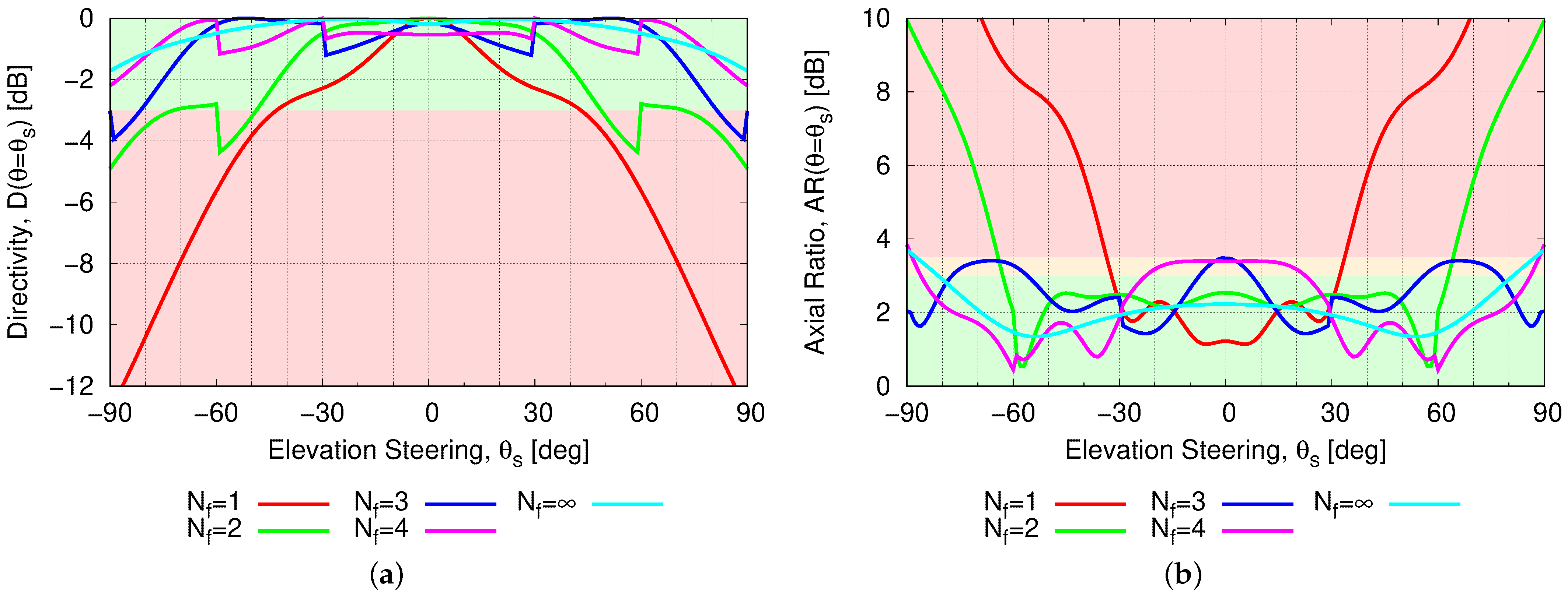
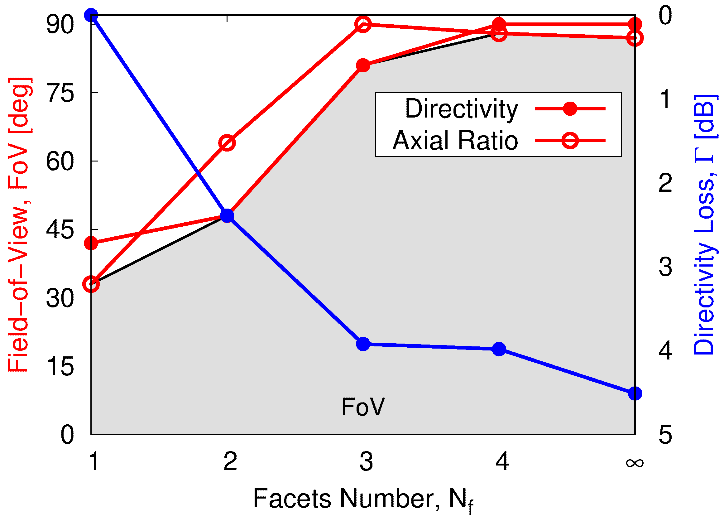
4.1. The Faceted Linear Array

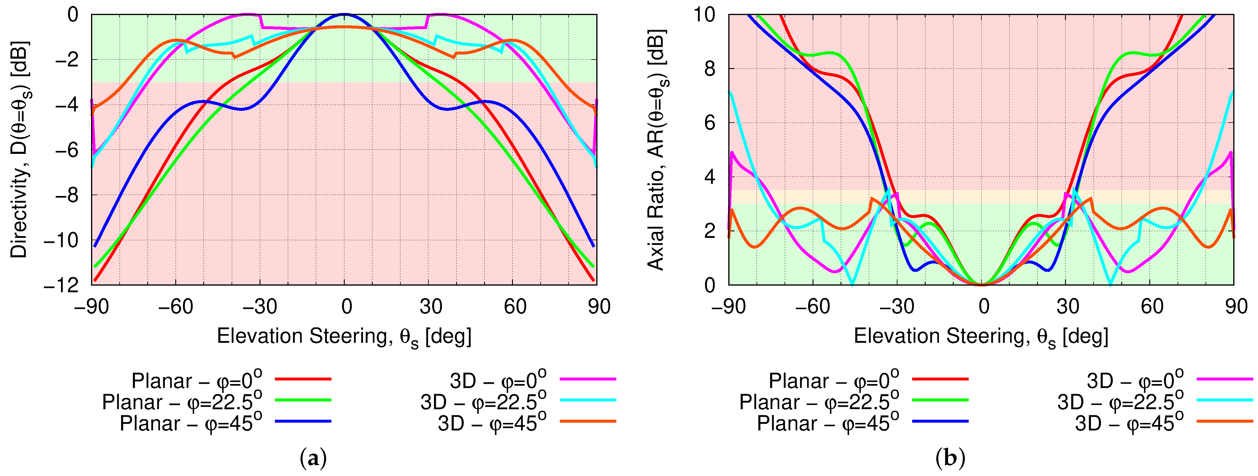
A trade-off study on a linear faceted array is conducted on different geometries depicted in Figure 8. Starting from a linear array ($N_f=1$), Figure 8a, the number of facets $N_f$ incrementally increases by reaching the full conformal aperture in Figure 8e ($N_f=\infty$).

In Figure 8, the elements are represented in red when a rotation of ${180}^{°}$ is applied for symmetrical steering, compensating for the non-ideal far field of the element pattern. All the geometries involve $N=60$ elements, which is the simplification of the $60\times 60$ reference planar array presented in Figure 9a.

The evaluated performances are depicted in Figure 10a,b, respectively, for the directivity and axial ratio FoV. Directivity and axial ratio are depicted at the steering direction, $D\left(\theta ={\theta }_s,\phi =0\right)$ and $AR\left(\theta ={\theta }_s,\phi =0\right)$. In

Table 2. Summary of the array performance for the faceted linear case.

Geometry	${\mathit{N}}_{\mathit{f}}$	Field of View (deg)			Directivity Loss, $\Gamma$ (dB)
		Directivity	Axial Ratio	Total
Linear	1	$\pm 42$	$\pm 33$	$\pm 33$	0
Triangular	2	$\pm 48$	$\pm 64$	$\pm 48$	$2.39$
Trapezoidal	3	$\pm 81$	$\pm 90$	$\pm 81$	$3.92$
4-Segment	4	$\pm 90$	$\pm 88$	$\pm 88$	$3.98$
Conformal	∞	$\pm 90$	$\pm 87$	$\pm 87$	$4.51$

, a complete list of the main values is presented. It is worth mentioning that for $N_f=1$ (the linear case), the steering is equivalent to the element pattern which is limiting the FoV to $\pm {42}^{°}$. An axial ratio, $AR\left(\theta ={\theta }_s,\phi =0\right)\le 3.5$ dB, is achieved within the FoV $\pm {33}^{°}$. Beyond this range, degraded performance would significantly impact the partial directivity of the array (e.g., LHCP/RHCP components).

As the number of facets is increased ($N_f>1$), jumps in the normalized directivity during steering occur. These jumps result from clusters of elements being turned on when the condition for steering direction, explained in Section 3.3.1, is met. However, directivity FoV significantly improves already at $N_f=2$ (the triangular case) with $\pm {48}^{°}$ and axial ratio FoV $\pm {64}^{°}$. Due to the tilted position of the elements, a directivity loss of $\Gamma =2.39$ dB is recorded with respect to the linear array (the reference case).

At $N_f=3$, a trapezoidal geometry is considered, expanding directivity FoV to $\pm {81}^{°}$ and axial ratio FoV to $\pm {90}^{°}$. The overall directivity loss, compared to the linear case, is equivalent to $\Gamma =3.92$ dB. In the case of a four-segment array at $N_f=4$, the simulated directivity FoV is equivalent to $\pm {99}^{°}$ which is more than the required $\pm {90}^{°}$. However, since the array is considered installed on a ground metal platform (e.g., the aircraft fuselage), scan range above $\pm {90}^{°}$ is not here considered. Additionally, axial ratio FoV is $\pm {88}^{°}$, and a directivity loss of $\Gamma =3.98$ dB is observed. Indeed, increasing the conformity of the structure (e.g., increasing $N_f$) keeps the radiated beam constant over a larger angular range, leading to a clear reduction in the maximum achievable value. As proof, in the conformal scenario $N_f=\infty$, directivity FoV is again above the $\pm {90}^{°}$ range, the axial ratio FoV is $\pm {87}^{°}$, and the maximum achievable directivity is reduced to $\Gamma =4.51$ dB.

Regarding the decrement in the axial ratio FoV for $N_f=4$ and $N_f=\infty$, this is easily explained by Figure 10b. By looking at $N_f=3$ (blue line), $N_f=4$ (magenta line) and $N_f=\infty$ (cyan line), the conformal geometry is the one exhibiting a better uniformity along the elevation steering range. The axial ratio starts to diverge only close to the horizon level (${\theta }_s={90}^{°}$) as expected.

Concluding, in Figure 11, directivity and axial ratio FoV (on the left y-axis in red) are depicted vs. the number of facets $N_f$ (x-axis). On the right y-axis in blue, directivity loss $\Gamma$ is shown. The best architecture is the one which satisfies the multiple objectives: maximization of directivity and axial ratio FoV, minimization of the number of facets $N_f$ (which is translated in manufacturing complexity) and minimization of directivity loss $\Gamma$. Among all the possible solutions, trapezoidal geometry ($N_f=3$) is selected for the expansion to the 3D case by weighting the different objectives considered.

4.2. The 3D Array

In Figure 9a, the reference planar array is shown. As previously mentioned in Section 2, it is composed of $60\times 60$ elements spaced at $\lambda /2$ and it achieves a directivity of $42.3$ dBiC (LHCP), depicted in Figure 9b. The elements of the array are properly rotated for symmetry in the scan range and the phase is then compensated through the ${\psi }_n$ term in (12).

The selected trapezoidal geometry in Figure 8c is expanded to the 3D case to enable 2D steering, similarly to [37]. The total number of facets is therefore increased to $N_f=5$. In the following, two different geometries, shown in Figure 12, are analyzed. Indeed, for the 3D case, the number of elements for each facets is adapted and this can be obtained either by keeping the number of elements similar to the planar case (configuration T1 in Figure 12a) or by fully using the available footprint of the planar array (configuration T2 in Figure 12b). For T1 configuration, the 3D array is created by a $3\times 24$ linear array and resulting in 3936 elements in the aperture. If considered the $3\times 20$ linear array, as for the linear case, the overall number of elements would be much smaller than 3600. When the footprint of the planar reference array is considered (configuration T2), a linear array with $3\times 30$ elements is considered for the expansion to the 3D case. In this case, the total number of elements in the aperture is 6180. This solution will be latter investigated to compensate for any directivity losses with respect to the planar case.

Also in this scenario, the array elements are opportunely rotated for symmetry in the scanning. In Figure 12, the colors of array elements represent the respective rotation which is compensated by the ${\psi }_n$ term in the phase computation in (12). It is worth to mention that both the geometries, T1 and T2, fit into the footprints foreseen in commercial aircraft fuselages as in [38].

The $N_f=5$ planar PCBs can conveniently host the required amount of beamformer ICs for controlling in amplitude and phase all the elements of the array face. A 5:1 power combiner can be implemented at the bottom of the structure.

The steering performance is evaluated once again with an elevation steering resolution of $1^{°}$ in the upper hemisphere ${\theta }_s\in \left[0^{°},{90}^{°}\right]$. Regarding the azimuth steering, in Figure 13, the cases for ${\phi }_s=\left\{0^{°},22.5^{°},{45}^{°}\right\}$ are shown. Other azimuth angles for ${\phi }_s>{45}^{°}$ would be symmetrical for the rotation of the elements. In

Table 3. Summary of performances for the 2 configurations of 3D array vs. the reference planar array.

Geometry	${\mathit{N}}_{\mathit{f}}$	N	Scan Range (deg)			Directivity Loss, $\Gamma$ (dB)	Max Directivity (dBiC)
			Directivity	Axial Ratio	Total
Planar	∞	3600	$\pm 24$	$\pm 31$	$\pm 24$	0	$42.3$
3D T1	5	3936	$\pm 70$	$\pm 76$	$\pm 70$	$4.75$	$37.55$
3D T2	5	6180	$\pm 70$	$\pm 76$	$\pm 70$	$2.79$	$39.51$

, a summary of performances for the 3D arrays (configuration T1 and T2) vs. the reference planar array are listed.

As expected, looking at directivity FoV in Figure 13a for the planar reference case, symmetrical steering limited to the element pattern is achieved (red, green and blue lines). At $\phi ={45}^{°}$, the worst performances are recorded, limiting directivity FoV to $\pm {24}^{°}$. Axial ratio FoV in Figure 13b performs slightly better in the $\pm {31}^{°}$ range. As previously stated, the maximum LHCP directivity among all the steering angles is $42.3$ dBiC. It is used as reference value for computing directivity loss $\Gamma$ for the 3D array.

For the 3D array, only T1 is shown in Figure 13, since T2 is a scaled version of T1 and the same performances were simulated. Overall, the array has directivity FoV of $\pm {70}^{°}$ in the worst case for ${\phi }_s=0^{°}$ (violet line). Directivity FoV for the best case when ${\phi }_s={45}^{°}$ is $\pm {77}^{°}$. The reduction in directivity FoV with respect to the linear case ($\pm {81}^{°}$) is explained by the fact that the 3D array is not conformal in the azimuth. Although not exactly matching the performance obtained in the linear case, configuration T1 still shows a remarkable improvement from the planar case, considerably extending the directivity and total field of view of $\pm {46}^{°}$. Moreover, axial ratio FoV is also strongly improved from $\pm {31}^{°}$ of the planar array to $\pm {76}^{°}$.

Analyzing directivity loss $\Gamma$, T1 has a maximum directivity of $37.55$ dBiC which is translated in a loss of $\Gamma =4.75$ dB. Discussing these results, the planar reference array has higher directivity at zenith but also higher scan losses through the scan range. From a link budget perspective, the maximum throughput is higher for the reference case, but it is reduced strongly as soon as the steering angle diverges from zenith, causing a drop in performances. On the other hand, the presented 3D architecture has a lower throughput due to the loss in the directivity but constant performance in the extended FoV region. A bigger array, T2, in Figure 12b is therefore built by considering the footprint of the planar array. As previously mentioned, the number of elements is increased to $N=6180$. Same performances are found for the T2 case with directivity loss reduced to $2.79$ dB and a maximum directivity of $39.51$ dBiC, which is very close to the original requirements of 40 dBiC.

As last, in Figure 14, the FoV map for both directivity (Figure 14a,c) and axial ratio (Figure 14b,d) is shown. The contour highlights the requirements of $-3$ dB for the directivity scan loss and $3.5$ dB for the axial ratio. The achieved total FoV for both the architectures is depicted through the red rectangle, $\pm {24}^{°}$ for the planar and $\pm {70}^{°}$ for the 3D array.

In Figure 15, it can be clearly noticed how the achieved FoV is strongly broadened for the 3D array. As an example, spherical directivity LHCP at ${\theta }_s={70}^{°}$ and ${\phi }_s={45}^{°}$ is shown for the planar and 3D array in T2 configuration. In the zoom area, the spherical directivity is normalized with respect to its maximum among all the steering angles ($42.3$ dBiC for the planar array and $39.51$ dBiC for the 3D T2 array). Contour lines are depicted every $-3,-10,-20$ dB to highlight the directivity roll-off. Even if in the 3D architecture the pointing angle is not fully centered in the $-3$ dB region, the beam shape is still well symmetric. On the other hand, in the planar array the beam is strongly wider and not anymore in the desirable $-3$ dB region.

5. Conclusions

In this paper, a 3D array for enhancing the FoV of phased arrays for mobility applications is presented. FoV is computed by considering both directivity and axial ratio with a requirement of 3 dB of scan loss and maximum axial ratio of $3.5$ dB.

Conformal array are an easy and efficient solution for improving the FoV. While the ideal conformal shape is challenging to manufacture, faceted solutions are investigated with the goal to enhance the FoV while keeping minimized the number of facets. An analysis on different linear faceted arrays permits to find the best candidate for improving FoV. The case for $N_f=3$ is chosen for building a 3D array.

The proposed 3D solution permits to improve the directivity and total FoV from $\pm {24}^{°}$ to $\pm {70}^{°}$ with a reduced number of facets ($N_f=5$). Also, axial ratio FoV is significantly improved from $\pm {31}^{°}$ of the planar reference case to $\pm {76}^{°}$ of the 3D array. Overall, the total FoV is increased by $\pm {46}^{°}$. The solution can be manufactured through planar PCBs avoiding complex and costly dedicated manufacturing.

As proof-of-concept, the 3D array is demonstrated for the Ka-band in receive mode, but analogous solutions can be achieved in other frequency bands. Specially, multi-band antennas able to support both the transmitter and receive part would be beneficial for avoiding shadow between the arrays and maximally exploiting the benefits of the 3D arrangement.

References

1. European Telecommunications Standards Institute; Satellite Earth Stations and Systems (SES). Technical Report on Antenna Performance Characterization for GSO Mobile Applications; Technical Report TR 103 233 V1.1.1; European Telecommunications Standards Institute: Sophia Antipolis, France, 2016. [Google Scholar]
2. Yang, G.; Li, J.; Wei, D.; Xu, R. Study on Wide-Angle Scanning Linear Phased Array Antenna. IEEE Trans. Antennas Propag. 2018, 66, 450–455. [Google Scholar] [CrossRef]
3. Yang, G.; Li, J.; Zhou, S.G.; Qi, Y. A Wide-Angle E-Plane Scanning Linear Array Antenna with Wide Beam Elements. IEEE Antennas Wirel. Propag. Lett. 2017, 16, 2923–2926. [Google Scholar] [CrossRef]
4. Wang, R.; Wang, B.Z.; Hu, C.; Ding, X. Wide-angle scanning planar array with quasi-hemispherical-pattern elements. Sci. Rep. 2017, 7, 2729. [Google Scholar] [CrossRef] [PubMed]
5. Cheng, Y.F.; Ding, X.; Shao, W.; Yu, M.X.; Wang, B.Z. 2-D Planar Wide-Angle Scanning-Phased Array Based on Wide-Beam Elements. IEEE Antennas Wirel. Propag. Lett. 2017, 16, 876–879. [Google Scholar] [CrossRef]
6. Ahn, B.; Hwang, I.J.; Kim, K.S.; Chae, S.C.; Yu, J.W.; Lee, H.L. Wide-Angle Scanning Phased Array Antenna using High Gain Pattern Reconfigurable Antenna Elements. Sci. Rep. 2019, 9, 18391. [Google Scholar] [CrossRef]
7. Bai, Y.Y.; Xiao, S.; Tang, M.C.; Ding, Z.F.; Wang, B.Z. Wide-Angle Scanning Phased Array with Pattern Reconfigurable Elements. IEEE Trans. Antennas Propag. 2011, 59, 4071–4076. [Google Scholar] [CrossRef]
8. Ding, X.; Cheng, Y.F.; Shao, W.; Li, H.; Wang, B.Z.; Anagnostou, D.E. A Wide-Angle Scanning Planar Phased Array with Pattern Reconfigurable Magnetic Current Element. IEEE Trans. Antennas Propag. 2017, 65, 1434–1439. [Google Scholar] [CrossRef]
9. Federico, G.; Song, Z.; Theis, G.; Caratelli, D.; Smolders, A.B. Multi-Mode Antennas for Ultra-Wide-Angle Scanning Millimeter-Wave Arrays. IEEE Open J. Antennas Propag. 2023, 4, 912–923. [Google Scholar] [CrossRef]
10. Ji, B.; Yang, G. Wide-Angle Scanning Phased Array Antenna. In Proceedings of the 2019 IEEE International Symposium on Antennas and Propagation and USNC-URSI Radio Science Meeting, Atlanta, GA, USA, 7–12 July 2019; pp. 2065–2066. [Google Scholar] [CrossRef]
11. Yang, G.; Li, J.; Xu, R.; Ma, Y.; Qi, Y. Improving the Performance of Wide-Angle Scanning Array Antenna with a High-Impedance Periodic Structure. IEEE Antennas Wirel. Propag. Lett. 2016, 15, 1819–1822. [Google Scholar] [CrossRef]
12. Yang, G.; Zhang, Y.; Zhang, S. Wide-Band and Wide-Angle Scanning Phased Array Antenna for Mobile Communication System. IEEE Open J. Antennas Propag. 2021, 2, 203–212. [Google Scholar] [CrossRef]
13. Yun, J.; Park, D.; Jang, D.; Hwang, K.C. Design of an Active Beam-Steering Array with a Perforated Wide-Angle Impedance Matching Layer. IEEE Trans. Antennas Propag. 2021, 69, 6028–6033. [Google Scholar] [CrossRef]
14. Hu, C.H.; Wang, B.Z.; Gao, G.F.; Wang, R.; Xiao, S.Q.; Ding, X. Conjugate Impedance Matching Method for Wideband and Wide-Angle Impedance Matching Layer with 70° Scanning in the H-Plane. IEEE Antennas Wirel. Propag. Lett. 2021, 20, 63–67. [Google Scholar] [CrossRef]
15. Gandini, E.; Silvestri, F.; Benini, A.; Gerini, G.; Martini, E.; Maci, S.; Viganò, M.C.; Toso, G.; Monni, S. A Dielectric Dome Antenna with Reduced Profile and Wide Scanning Capability. IEEE Trans. Antennas Propag. 2021, 69, 747–759. [Google Scholar] [CrossRef]
16. Sun, F.; Zhang, S.; He, S. A General Method for Designing a Radome to Enhance the Scanning Angle of a Phased Array Antenna. Prog. Electromagn. Res. 2014, 145, 203–212. [Google Scholar] [CrossRef]
17. Sun, F.; He, S. Extending the scanning angle of a phased array antenna by using a null-space medium. Sci. Rep. 2014, 4, 6832. [Google Scholar] [CrossRef]
18. Josefsson, L.; Persson, P. Conformal Array Antenna Theory and Design; John Wiley and Sons, Inc.: Hoboken, NJ, USA, 2016. [Google Scholar]
19. Boulos, F.; Elmarissi, W.; Caizzone, S. A GNSS Conformal Antenna Achieving Hemispherical Coverage in L1/L5 Band. In Proceedings of the 2022 16th European Conference on Antennas and Propagation (EuCAP), Madrid, Spain, 27 March–1 April 2022; pp. 1–4. [Google Scholar] [CrossRef]
20. Xiao, S.; Yang, S.; Zhang, H.; Xiao, Q.; Chen, Y.; Qu, S.W. Practical Implementation of Wideband and Wide-Scanning Cylindrically Conformal Phased Array. IEEE Trans. Antennas Propag. 2019, 67, 5729–5733. [Google Scholar] [CrossRef]
21. Kim, Y.B.; Lim, S.; Lee, H.L. Electrically Conformal Antenna Array with Planar Multipole Structure for 2-D Wide Angle Beam Steering. IEEE Access 2020, 8, 157261–157269. [Google Scholar] [CrossRef]
22. Xu, H.; Zhang, B.z.; Duan, J.p.; Cui, J.; Xu, Y.; Tian, Y.; Yan, L.; Xiong, M.; Jia, Q. Wide Solid Angle Beam-Switching Conical Conformal Array Antenna With High Gain for 5G Applications. IEEE Antennas Wirel. Propag. Lett. 2018, 17, 2304–2308. [Google Scholar] [CrossRef]
23. Pfeiffer, C.; Massman, J. A UWB Low-Profile Hemispherical Array for Wide Angle Scanning. IEEE Trans. Antennas Propag. 2023, 71, 508–517. [Google Scholar] [CrossRef]
24. Knott, P. Design and Experimental Results of a Spherical Antenna Array for a Conformal Array Demonstrator. In Proceedings of the 2007 2nd International ITG Conference on Antennas, Munich, Germany, 28–30 March 2007; pp. 120–123. [Google Scholar] [CrossRef]
25. Knittel, G. Choosing the number of faces of a phased-array antenna for hemisphere scan coverage. IEEE Trans. Antennas Propag. 1965, 13, 878–882. [Google Scholar] [CrossRef]
26. Kmetzo, J. An analytical approach to the coverage of a hemisphere by n planar phased arrays. IEEE Trans. Antennas Propag. 1967, 15, 367–371. [Google Scholar] [CrossRef]
27. Tomasic, B.; Turtle, J.; Liu, S.; Schmier, R.; Bharj, S.; Oleski, P. The geodesic dome phased array antenna for satellite control and communication-subarray design, development and demonstration. In Proceedings of the IEEE International Symposium on Phased Array Systems and Technology, Boston, MA, USA, 14–17 October 2003; pp. 411–416. [Google Scholar] [CrossRef]
28. Munno, F. Conformal Array Geometry for Hemispherical Coverage. Electronics 2021, 10, 903. [Google Scholar] [CrossRef]
29. Boulos, F.; Riemschneider, G.F.; Caizzone, S. 3D Phased Array Architecture for Field-of-View Enhancement in Satcom COTM Terminals. In Proceedings of the 2023 IEEE International Symposium on Antennas and Propagation and USNC-URSI Radio Science Meeting (USNC-URSI), Portland, OR, USA, 23–28 July 2023. [Google Scholar] [CrossRef]
30. Adithyababu, A.P.T.; Boulos, F.; Caizzone, S. Analysis of user terminal trade-offs for future satellite communication applications. In Proceedings of the 27th Ka and Broadband Communications Conference, Stresa, Italy, 18–21 October 2022. [Google Scholar]
31. Riemschneider, G.F. Analysis of Bandwidth and Field-of-View Improvement Techniques for Satellite Communication Phased Arrays in Ka Band. Master’s Thesis, Institute of High-Frequency Technology, Technische Universität Hamburg (TUHH), Hamburg, Germany, 2022. [Google Scholar]
32. Recommendation ITU-R V.431-8 (08/2015) Nomenclature of the Frequency and Wavelength Bands Used in Telecommunications. Available online: https://www.itu.int/dms_pubrec/itu-r/rec/v/R-REC-V.431-8-201508-I!!PDF-E.pdf (accessed on 11 December 2023).
33. Host, N.K.; Ricciardi, G.F.; Krichene, H.A.; Ho, M.T. A Sine-Space, Mixed-Coordinate Polarization Representation for Rotated Phased Arrays: Using a linear algebra calculus to transform radiated fields. IEEE Antennas Propag. Mag. 2022, 64, 71–81. [Google Scholar] [CrossRef]
34. Milligan, T.A. Modern Antenna Design; John Wiley and Sons, Inc.: Hoboken, NJ, USA, 2005. [Google Scholar]
35. Haupt, R.L. Antenna Arrays: A Computational Approach; Wiley: Hoboken, NJ, USA, 2010. [Google Scholar]
36. Balanis, C.A. Antenna Theory: Analysis and Design; John Wiley and Sons, Inc.: Hoboken, NJ, USA, 2016. [Google Scholar]
37. Khalifa, I.; Vaughan, R.G. Geometric Design and Comparison of Multifaceted Antenna Arrays for Hemispherical Coverage. IEEE Trans. Antennas Propag. 2009, 57, 2608–2614. [Google Scholar] [CrossRef]
38. Carlisle Interconnect Technologies. FlightGear™ ARINC 791. 2021. Available online: https://www.carlisleit.com/markets/commercial-aerospace/ifeci/connectivity-kits/arinc-791-universal-installation-solutions/ (accessed on 3 January 2024).
Figure 1. Pictorial representation of a satcom terminal suffering from limited FoV in mobility applications: (a) the satellite is within the FoV of the satcom terminal, (b) the satcom terminal loses connectivity with the established satellite while in motion, requiring a handover to another satellite.
Electronics 13 00310 g001
Figure 2. Flowchart of the directivity computation for a 3D array.
Electronics 13 00310 g002
Figure 3. Sketch of the spherical coordinate system.
Electronics 13 00310 g003
Figure 4. HFSS model of the patch antenna working in the receive Ka frequency band and used as element pattern for the array computation.
Electronics 13 00310 g004
Figure 5. Realized gain of the patch antenna for both LHCP and RHCP at φ = 0 ° (red and blue lines) and φ = 90 ° (green and magenta lines).
Electronics 13 00310 g005
Figure 6. Example representing the cluster of elements activated while the array is steering: (a) all the elements are activated, (b) only a cluster of elements is turned on.
Electronics 13 00310 g006
Figure 7. Rotation of the antennas for compensating the asymmetry of the non-ideal element pattern in a linear array.
Electronics 13 00310 g007
Figure 8. Geometries of the different faceted arrays considered in this analysis. The geometries are listed for number of facets N f starting by the (a) linear case N f = 1 , (b) triangular N f = 2 , (c) trapezoidal N f = 3 , (d) 4 segment N f = 4 and ending with the (e) fully conformal scenario N f = .
Electronics 13 00310 g008
Figure 9. (a) Geometry and (b) directivity of the reference 60 × 60 planar array for the boresight case. The different colors in (a) represent the different azimuth orientations of the elements.
Electronics 13 00310 g009
Figure 10. Summary of the array performance for the different 1D faceted arrays considered: (a) Directivity vs. steering and (b) axial ratio vs. steering.
Electronics 13 00310 g010
Figure 11. Directivity FoV, axial ratio FoV and directivity loss Γ vs. the number of facets N f . In red on the left y-axis, the directivity and axial ratio FoV is depicted, while in blue on the right y-axis, the directivity loss Γ is depicted.
Electronics 13 00310 g011
Figure 12. Three-dimensional faceted array based on the trapezoidal geometry for (a) T1 and (b) T2 configurations.
Electronics 13 00310 g012
Figure 13. (a) Directivity and (b) axial ratio FoV for θ s 0 ° , 90 ° and φ = 0 ° , 22 . 5 ° , 90 ° .
Electronics 13 00310 g013
Figure 14. (a,c) Directivity and (b,d) axial ratio map vs. steering in elevation and azimuth for the (a,b) planar array and for the (c,d) 3D array T2. The contour highlights the requirement 3 dB for the directivity and 3.5 dB for axial ratio. The red square highlights the achieved FoV.
Electronics 13 00310 g014
Figure 15. Spherical directivity at θ s = 70 ° and φ s = 45 ° for (a) planar array and (b) 3D array for T2 configuration. The zoom is normalized with respect to its maximum along all the steering angles.
Electronics 13 00310 g015