
Deep Learning-Based Detection Algorithm for the Multi-User MIMO-NOMA System

 , ,
, ,  and
and
Abstract
1. Introduction
2. System Model
2.1. NOMA System
2.2. SIC Receiver
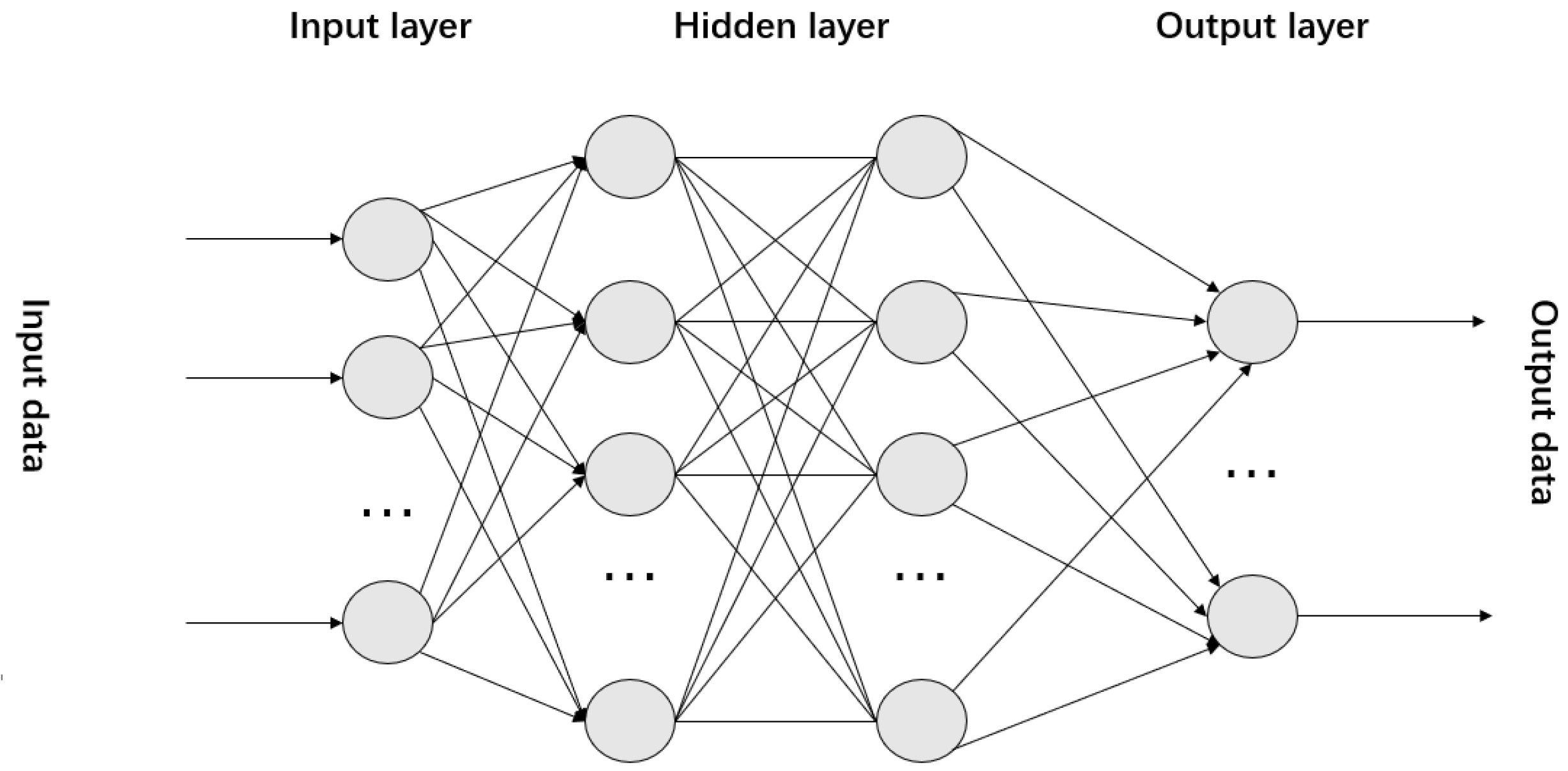
2.3. DNN Network
3. Proposed Method
3.1. MIMO-NOMA System
3.2. FDNN Model
3.2.1. Data Preprocessing
3.2.2. Detection Module
3.2.3. Feedback Module
3.2.4. Model Training
4. Simulation Results
4.1. Data Set
4.2. Hidden Layers
4.3. Batch Size
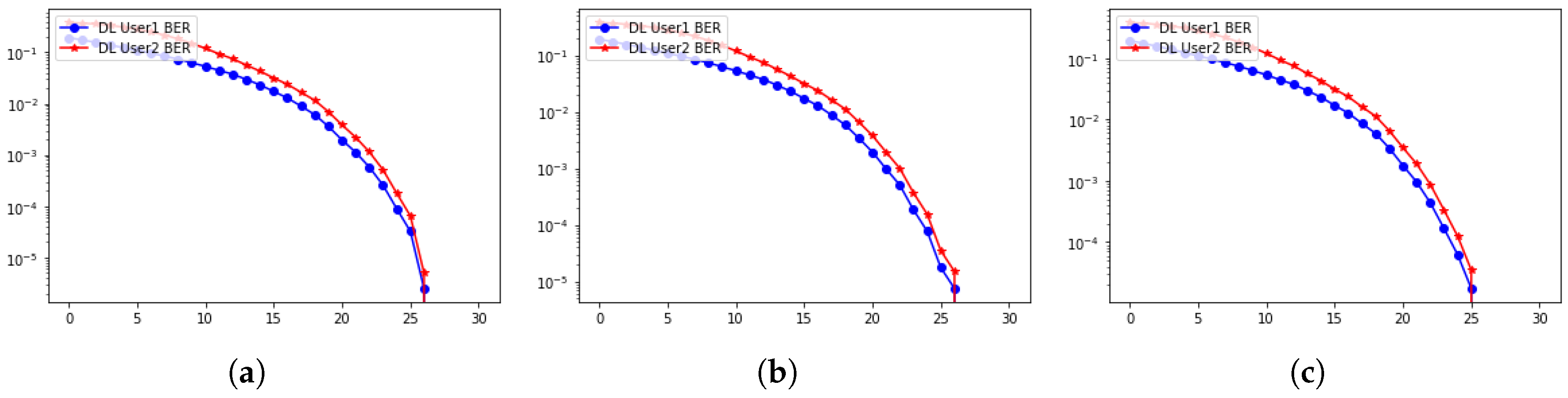
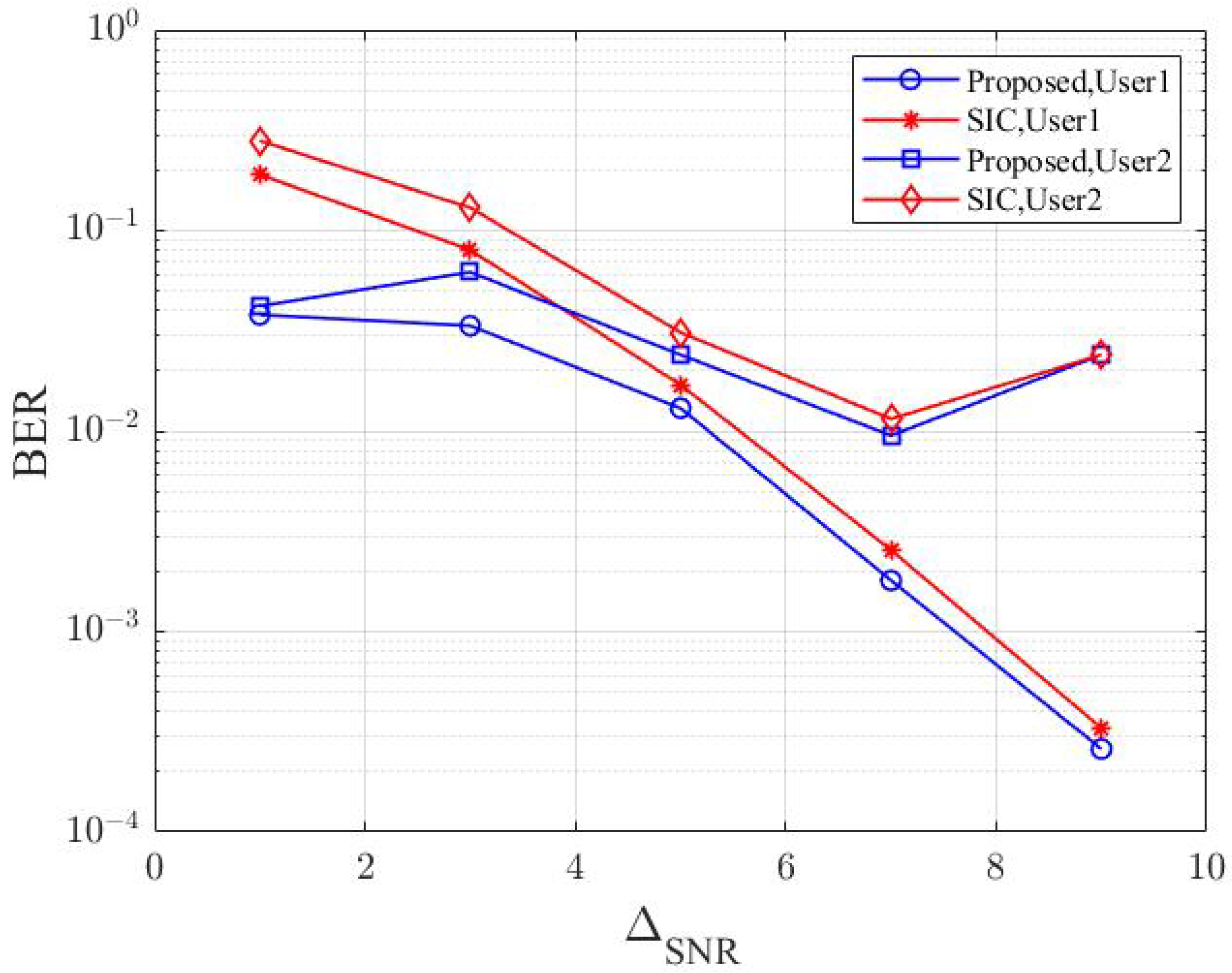
4.4. Performance of FDNN Receivers
5. Conclusions
Author Contributions
Funding
Data Availability Statement
Conflicts of Interest
References
- Saad, W.; Bennis, M.; Chen, M. A Vision of 6G Wireless Systems: Applications, Trends, Technologies, and Open Research Problems. IEEE Netw. 2020, 34, 134–142. [Google Scholar] [CrossRef]
- Zhang, H.; Zhou, T.; Xu, T.; Hu, H. Remote Interference Discrimination Testbed Employing AI Ensemble Algorithms for 6G TDD Networks. Sensors 2023, 23, 2264. [Google Scholar] [CrossRef] [PubMed]
- Akyildiz, I.F.; Kak, A.; Nie, S.T. 6G and Beyond: The Future of Wireless Communications Systems. IEEE Access 2020, 8, 133995–134030. [Google Scholar] [CrossRef]
- Wu, J.; Xu, T.; Zhou, T.; Chen, X.; Zhang, N.; Hu, H. Feature-Based Spectrum Sensing of NOMA System for Cognitive IoT Networks. IEEE Internet Things J. 2023, 10, 801–814. [Google Scholar] [CrossRef]
- Saito, Y.; Kishiyama, Y.; Benjebbour, A.; Nakamura, T.; Li, A.; Higuchi, K. Non-Orthogonal Multiple Access (NOMA) for Cellular Future Radio Access. In Proceedings of the IEEE 77th Vehicular Technology Conference (VTC Spring), Dresden, Germany, 2–5 June 2013. [Google Scholar]
- Ding, Z.; Lei, X.; Karagiannidis, G.K.; Schober, R.; Yuan, J.; Bhargava, V.K. A Survey on Non-Orthogonal Multiple Access for 5G Networks: Research Challenges and Future Trends. IEEE J. Sel. Areas Commun. 2017, 35, 2181–2195. [Google Scholar] [CrossRef]
- Larsson, E.G.; Edfors, O.; Tufvesson, F.; Marzetta, T.L. Massive MIMO for next generation wireless systems. IEEE Commun. Mag. 2014, 52, 186–195. [Google Scholar] [CrossRef]
- Agiwal, M.; Roy, A.; Saxena, N. Next Generation 5G Wireless Networks: A Comprehensive Survey. IEEE Commun. Surv. Tutor. 2016, 18, 1617–1655. [Google Scholar] [CrossRef]
- Tweneboah-Koduah, S.; Affum, E.A.; Agyekum, K.A.P.; Ajagbe, S.A.; Adigun, M.O. Performance of Cooperative Relay NOMA with Large Antenna Transmitters. Electronics 2022, 11, 3482. [Google Scholar] [CrossRef]
- Alraddady, F.; Ahmed, I.; Habtemicail, F. Robust Hybrid Beam-Forming for Non-Orthogonal Multiple Access in Massive MIMO Downlink. Electronics 2022, 11, 75. [Google Scholar] [CrossRef]
- Gkonis, P.K.; Trakadas, P.T.; Sarakis, L.E. Non-Orthogonal Multiple Access in Multiuser MIMO Configurations via Code Reuse and Principal Component Analysis. Electronics 2020, 9, 1330. [Google Scholar] [CrossRef]
- Sur, S.N.; Kandar, D.; Silva, A.; Nguyen, N.D.; Nandi, S.; Do, D.T. Hybrid Precoding Algorithm for Millimeter-Wave Massive MIMO-NOMA Systems. Electronics 2022, 11, 2198. [Google Scholar] [CrossRef]
- Xie, W.L.; Ding, X.; Cai, B.W.; Li, X.; Wei, M.S. Downlink MIMO-NOMA System for 6G Internet of Things. Electronics 2022, 11, 3233. [Google Scholar] [CrossRef]
- El-Gayar, M.M.; Ajour, M.N. Resource Allocation in UAV-Enabled NOMA Networks for Enhanced Six-G Communications Systems. Electronics 2023, 12, 5033. [Google Scholar] [CrossRef]
- Dai, L.L.; Wang, B.C.; Yuan, Y.F.; Han, S.F.; Chih-Lin, I.; Wang, Z.C. Non-Orthogonal Multiple Access for 5G: Solutions, Challenges, Opportunities, and Future Research Trends. IEEE Commun. Mag. 2015, 53, 74–81. [Google Scholar] [CrossRef]
- Mohsan, S.A.H.; Li, Y.; Shvetsov, A.V.; Varela-Aldás, J.; Mostafa, S.M.; Elfikky, A. A Survey of Deep Learning Based NOMA: State of the Art, Key Aspects, Open Challenges and Future Trends. Sensors 2023, 23, 2946. [Google Scholar] [CrossRef]
- Li, J.; Gao, T.; He, B.; Zheng, W.; Lin, F. Power Allocation and User Grouping for NOMA Downlink Systems. Appl. Sci. 2023, 13, 2452. [Google Scholar] [CrossRef]
- Gaballa, M.; Abbod, M.; Aldallal, A. Investigating the Combination of Deep Learning for Channel Estimation and Power Optimization in a Non-Orthogonal Multiple Access System. Sensors 2022, 22, 3666. [Google Scholar] [CrossRef]
- Dang, H.P.; Nguyen, M.S.V.; Do, D.T.; Nguyen, M.H.; Pham, M.T.; Kim, A.T. Secure Performance Analysis of Aerial RIS-NOMA-Aided Systems: Deep Neural Network Approach. Electronics 2022, 11, 2588. [Google Scholar] [CrossRef]
- Ryu, W.J.; Kim, J.W.; Kim, D.S. Resource Allocation in Downlink VLC-NOMA Systems for Factory Automation Scenario. Sensors 2022, 22, 9407. [Google Scholar] [CrossRef]
- Perdana, R.H.Y.; Nguyen, T.-V.; An, B. A Deep Learning-Based Spectral Efficiency Maximization in Multiple Users Multiple STAR-RISs Massive MIMO-NOMA Networks. In Proceedings of the 2023 Fourteenth International Conference on Ubiquitous and Future Networks (ICUFN), Paris, France, 4–7 July 2023. [Google Scholar]
- Shlezinger, N.; Fu, R.; Eldar, Y.C. DeepSIC: Deep Soft Interference Cancellation for Multiuser MIMO Detection. IEEE Trans. Wirel. Commun. 2021, 20, 1349–1362. [Google Scholar] [CrossRef]
- Chen, W.; Tang, Z. Research on improved receiver of NOMA-OFDM signal based on deep learning. In Proceedings of the 2021 International Conference on Communications, Information System and Computer Engineering (CISCE), Beijing, China, 14–16 May 2021. [Google Scholar]
- Sim, I.; Sun, Y.G.; Lee, D.; Kim, S.H.; Lee, J.; Kim, J.H.; Shin, Y.; Kim, J.Y. Deep Learning Based Successive Interference Cancellation Scheme in Nonorthogonal Multiple Access Downlink Network. Energies 2020, 13, 6237. [Google Scholar] [CrossRef]
- Gui, G.; Huang, H.J.; Song, Y.W.; Sari, H. Deep Learning for an Effective Nonorthogonal Multiple Access Scheme. IEEE Trans. Veh. Technol. 2018, 67, 8440–8450. [Google Scholar] [CrossRef]
- Kang, J.M.; Kim, I.; Chun, C.J. Deep Learning-Based MIMO-NOMA with Imperfect SIC Decoding. IEEE Syst. J. 2020, 14, 3414–3417. [Google Scholar] [CrossRef]
- Salama, W.M.; Aly, M.H.; Amer, E.S. Deep learning based BER improvement for NOMA-VLC systems with perfect and imperfect successive interference cancellation. Opt. Quantum Electron. 2023, 55, 692. [Google Scholar] [CrossRef]
- Ahmad, M.; Shin, S.Y. Wavelet-based massive MIMO-NOMA with advanced channel estimation and detection powered by deep learning. Phys. Commun. 2023, 61, 102189. [Google Scholar] [CrossRef]
- Islam, S.M.R.; Avazov, N.; Dobre, O.A.; Kwak, K.S. Power-Domain Non-Orthogonal Multiple Access (NOMA) in 5G Systems: Potentials and Challenges. IEEE Commun. Surv. Tutorials 2017, 19, 721–742. [Google Scholar] [CrossRef]
- Dai, L.L.; Wang, B.C.; Ding, Z.G.; Wang, Z.C.; Chen, S.; Hanzo, L. A Survey of Non-Orthogonal Multiple Access for 5G. IEEE Commun. Surv. Tutor. 2018, 20, 2294–2323. [Google Scholar] [CrossRef]
- Ding, Z.G.; Adachi, F.; Poor, H.V. The Application of MIMO to Non-Orthogonal Multiple Access. IEEE Trans. Wirel. Commun. 2016, 15, 537–552. [Google Scholar] [CrossRef]


| Parameters | Values |
|---|---|
| N | 2 |
| K | 2 |
| Modulation Mode | QPSK |
| Hidden Layers | 2 |
| Trainnig Sample Size | 200,000 |
| Regularization Parameter | 0.01 |
| Learning Rate | 0.02 |
| Batch Size | 100 |
| Epoch | 100 |
| User | ||
|---|---|---|
| User 1 for SIC | ||
| User 1 for FDNN | ||
| User 2 for SIC | ||
| User 2 for FDNN |
| User | |||
|---|---|---|---|
| User 1 for SIC | |||
| User 1 for FDNN | |||
| User 2 for SIC | |||
| User 2 for FDNN |
Disclaimer/Publisher’s Note: The statements, opinions and data contained in all publications are solely those of the individual author(s) and contributor(s) and not of MDPI and/or the editor(s). MDPI and/or the editor(s) disclaim responsibility for any injury to people or property resulting from any ideas, methods, instructions or products referred to in the content. |
© 2024 by the authors. Licensee MDPI, Basel, Switzerland. This article is an open access article distributed under the terms and conditions of the Creative Commons Attribution (CC BY) license (https://creativecommons.org/licenses/by/4.0/).
Share and Cite
Wang, Q.; Zhou, T.; Zhang, H.; Hu, H.; Pignaton de Freitas, E.; Feng, S. Deep Learning-Based Detection Algorithm for the Multi-User MIMO-NOMA System. Electronics 2024, 13, 255. https://doi.org/10.3390/electronics13020255
Wang Q, Zhou T, Zhang H, Hu H, Pignaton de Freitas E, Feng S. Deep Learning-Based Detection Algorithm for the Multi-User MIMO-NOMA System. Electronics. 2024; 13(2):255. https://doi.org/10.3390/electronics13020255
Chicago/Turabian StyleWang, Qixing, Ting Zhou, Hanzhong Zhang, Honglin Hu, Edison Pignaton de Freitas, and Songlin Feng. 2024. "Deep Learning-Based Detection Algorithm for the Multi-User MIMO-NOMA System" Electronics 13, no. 2: 255. https://doi.org/10.3390/electronics13020255
APA StyleWang, Q., Zhou, T., Zhang, H., Hu, H., Pignaton de Freitas, E., & Feng, S. (2024). Deep Learning-Based Detection Algorithm for the Multi-User MIMO-NOMA System. Electronics, 13(2), 255. https://doi.org/10.3390/electronics13020255