MPC-TD3 Trajectory Tracking Control for Electrically Driven Unmanned Tracked Vehicles

Abstract

To address the trajectory tracking issue of unmanned tracked vehicles, the majority of studies employ the Model Predictive Control (MPC). The MPC imposes high demands on model accuracy. Due to factors such as environmental interference, actuator constraints, and the nonlinearity of vehicles under high-speed conditions, dynamic and kinematic models fail to accurately delineate the motion process of tracked vehicles. Aiming at the problem of insufficient trajectory tracking precision of unmanned tracked vehicles, a trajectory tracking controller jointly controlled by the Twin Delayed Deep Deterministic policy gradient (TD3) algorithm and the MPC algorithm is developed. During offline training, the agent acquires the discrepancies between the model and the environment under various working conditions and optimizes its own network; during online reasoning, the agent adaptively compensates the output of the MPC based on the vehicle state. The experimental results indicate that, compared with the pure MPC algorithm, the MPC algorithm compensated based on the TD3 algorithm reduces the lateral errors by 41.67% and 22.55%, respectively, in circular and double-lane-change trajectory conditions.

1. Introduction

In recent years, with the application of electric drive technology for tracked vehicles, high-speed tracked vehicles have been evolving toward intelligence and unmanned operation. Electric drive tracked vehicles exhibit numerous advantages in control, such as precise torque control, rapid response speed, braking energy recovery, etc. [1,2]. For the control system, the motor serves as a precise actuator. This establishes the foundation for the unmanned operation of tracked vehicles. Regarding manned tracked vehicles, the driver achieves the vehicle’s tracking of the target road or trajectory by manipulating the steering wheel angle. The objective of the controller is to guarantee safety while precisely implementing the control quantity. The majority of studies have concentrated on vehicle stability control [3,4,5,6]. For unmanned tracked vehicles, the key technologies can be generalized as environmental perception, positioning and navigation, and decision making and planning, as well as trajectory tracking [7]. Whereas trajectory tracking, as the ultimate safeguard of the maneuverability and driving safety of unmanned tracked vehicles, demands high tracking precision.

The traditional approaches to trajectory tracking can be classified into three categories: geometry-based methods, model-free methods, and model-based methods. Pure pursuit (PP) and Stanley methods are geometry-based approaches. These two methods determine the front wheel steering angle command based on the geometric relationship between the vehicle and the desired trajectory. Ahn J et al. [8] and AbdElmoniem A et al. [9] verified the effectiveness of these two methods through experiments. Nevertheless, the control accuracy of geometry-based methods is not satisfactory under high-speed and off-road conditions. Among the model-free control methods, the PID algorithm is widely employed due to its simplicity and extensive application scope [10,11]. However, since its parameter tuning methods largely rely on experience, in trajectory tracking control, inappropriate parameters can lead to vehicle instability, entailing high test costs and time consumption. LQR and MPC algorithms are typical representatives of model-based methods. The quality of their control effects hinges on the accuracy of the model. Zhao Z et al. [12] enhanced the trajectory tracking accuracy of the vehicle by employing the method of optimizing the model. Through observing the slip and skid amounts of the tracks on both sides of the tracked vehicle via the extended Kalman filter, they were utilized as parameters to compensate for the model of the MPC controller.

In recent years, reinforcement learning has gradually been applied in the trajectory tracking control of vehicles. Srikonda S et al. [13] utilized the Deep Deterministic Policy Gradient (DDPG) algorithm in place of the traditional controller to realize vehicle trajectory tracking. Liu M et al. [14], in an attempt to enhance the training speed, initially employed data for the agent to undertake imitation learning, and subsequently conducted reinforcement learning to increase exploration, achieving trajectory tracking on urban roads in wheeled vehicles. However, for scenarios not encountered during the reinforcement learning training, the output actions of the agent can readily cause the vehicle to lose control. Hence, some scholars endeavor to combine reinforcement learning with traditional control algorithms. Shan Y et al. [15] employed the Proximal Policy Optimization (PPO) algorithm to regulate the output proportion of the PID algorithm and the PP algorithm, dynamically integrating the advantages of the two algorithms. Nevertheless, this method remains confined within the framework of traditional control methods. Wang S et al. [16] utilized Q-learning to compensate for the output of the PID algorithm, but the Q-learning method is suitable for control in discrete state spaces and would give rise to the dimension curse for continuous state spaces. Chen I M et al. [17] employed the PPO algorithm to compensate for the output of the PP algorithm, demonstrating excellent real-time performance.

In the domain of trajectory tracking of unmanned tracked vehicles, the majority of studies still adopt traditional control methods [18,19,20]. Nevertheless, there exist the following challenges in the control of high-speed tracked vehicles: On the one hand, the slip and skid between the tracks of high-speed tracked vehicles and the ground significantly increase, resulting in intensified nonlinear characteristics of the tracked vehicles. On the other hand, compared to the steering of wheeled vehicles, the differential steering response speed of tracked vehicles is slower. In response to the aforementioned challenges, this paper proposes the MPC-TD3 control method. Herein, the MPC controller provides the control quantity based on the simplified kinematic model of the tracked vehicle. For the portion where the kinematic model inaccurately describes the tracked vehicle model, the TD3 algorithm is employed to compensate for the output of the MPC controller.

2. Tracked Vehicle Model Construction

2.1. Kinematic Model of Tracked Vehicle

The global coordinate system $XOY$ and the vehicle body coordinate system $xoy$ are established as shown in Figure 1:

Figure 1. Kinematic model of tracked vehicle.

The position and attitude of the vehicle in the global coordinate system is $(X,Y,\theta )$, where $\theta$ is the heading angle of the tracked vehicle. In the local vehicle body coordinate system, $v_x,v_y,{\omega }_z$ are the longitudinal velocity, lateral velocity, and yaw rate of the vehicle, respectively; $o_c$ is the steering center of the tracked vehicle, $o_l$ is the instantaneous steering center of the left track of the tracked vehicle, and $o_r$ is the instantaneous steering center of the right track of the tracked vehicle. $(x_c,y_c),(x_l,y_l),(x_r,y_r)$ are the coordinates of these three points, respectively. These three points are on the same straight line, and this straight line intersects the left track and the right track at points $M$ and $N$, respectively. $v_s^l,v_s^r$ are the winding speeds of the left and right tracks, respectively; and $v_{Mq},v_{Nq}$ are the entrainment velocities of the vehicle body at points M and N, respectively.

Then the kinematic model of the tracked vehicle is:

$$\begin{array}{l}\left[\begin{array}{c}\dot{X}\\ \dot{Y}\\ \dot{\theta }\end{array}\right]=\left[\begin{array}{ccc}\cos \theta & -\sin \theta & 0\\ \sin \theta & \cos \theta & 0\\ 0& 0& 1\end{array}\right]\left[\begin{array}{c}{v}_x\\ v_y\\ {\omega }_z\end{array}\right]=\\ \left[\begin{array}{ccc}\cos \theta & -\sin \theta & 0\\ \sin \theta & \cos \theta & 0\\ 0& 0& 1\end{array}\right]\left[\begin{array}{c}{\displaystyle \frac{y_l{v}_s^r-y_r{v}_s^l}{y_l-y_r}}\\ {\displaystyle \frac{v_s^l-v_s^r}{y_l-y_r}}{x}_c\\ -{\displaystyle \frac{v_s^l-v_s^r}{y_l-y_r}}\end{array}\right]\end{array}$$

(1)

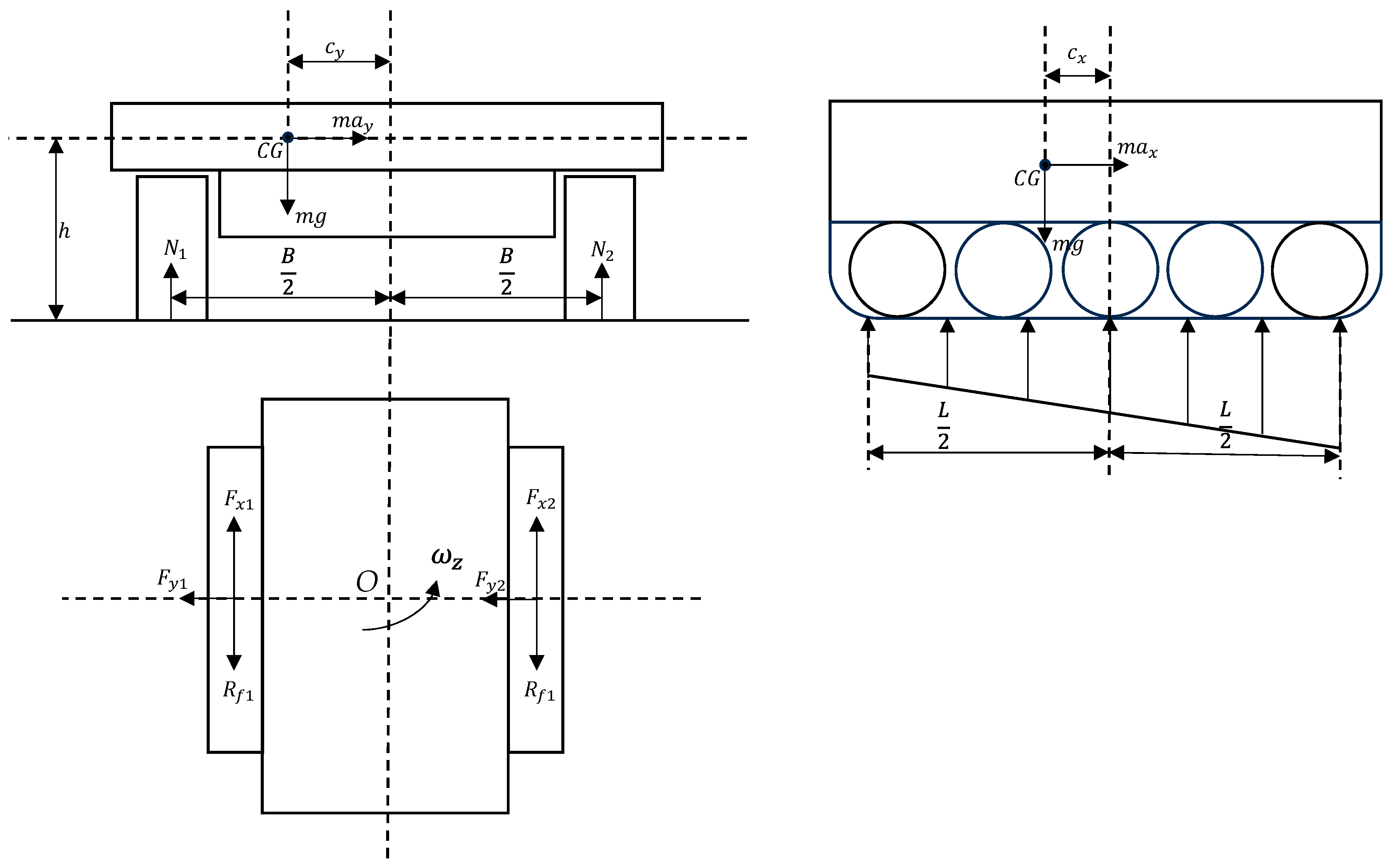
2.2. Dynamic Model of the Tracked Vehicle

The force diagram of the tracked vehicle is shown in Figure 2 as follows:

Figure 2. Dynamic model of the tracked vehicle.

The normal pressures imposed on the track plates on both sides of a tracked vehicle during steering can be represented as:

$$\begin{array}{l}{N}_l={\displaystyle \frac{1}{2}}mg-{\displaystyle \frac{m}{B}}(h({\dot{v}}_y+v_x{\omega }_z)-c_{y}g)\\ N_r={\displaystyle \frac{1}{2}}mg+{\displaystyle \frac{m}{B}}(h({\dot{v}}_y+v_x{\omega }_z)-c_{y}g)\\ P_{l,i}={\displaystyle \frac{N_1}{n}}-{\displaystyle \frac{6m}{L^{2}n}}(c_{x}g+h({\dot{v}}_x-v_y{\omega }_z))x_{li}\\ P_{r,i}={\displaystyle \frac{N_2}{n}}-{\displaystyle \frac{6m}{L^{2}n}}(c_{x}g+h({\dot{v}}_x-v_y{\omega }_z))x_{ri}\end{array}$$

(2)

where $N_l,N_r$ are the normal pressures exerted on the two sides of the tracks, respectively, $P_{li},P_{ri}$ are the pressures exerted on each track plate on the two sides, respectively, and $m$ is the mass of the tracked vehicle. $L$ is the grounding length of the track, $B$ is the center distance between the two sides of the tracks, $n$ is the number of track plates on the single side of the track, $c_x,c_y$ are the offsets of the center of mass of the tracked vehicle, respectively, and $x_{li},x_{ri}$ is the abscissa of each track plate in the vehicle coordinate system, respectively.

In the vehicle coordinate system, the coordinates of each track plate are:

$$\begin{array}{l}{x}_{ki}={\displaystyle \frac{L}{2}}-{\displaystyle {\int }_{t_{0}i}^t{v}_s^{k}r}\mathrm{d}t\\ y_{ki}=\mp {\displaystyle \frac{B}{2}}\end{array}$$

(3)

where $v_s^k$ is the winding speed of the $k$th side track, and $t_{0}i$ is the moment when this track plate begins to contact the ground.

The absolute velocities of each track plate are:

$$\begin{array}{l}{v}_{jx,ki}=v_s^k-(v_x\pm w_z({\displaystyle \frac{B}{2}}-c_y))\\ v_{jy,ki}=v_y-w_z(x_{ki}-c_x)\end{array}$$

(4)

Then, the shear displacement of each track plate is:

$$\begin{array}{l}{j}_{x,ki}={\displaystyle {\int }_{t_{0}i}^t{v}_{jx,ki}(\tau )}\mathrm{d}t\\ j_{y,ki}={\displaystyle {\int }_{t_{0}i}^t{v}_{jy,ki}(\tau )}\mathrm{d}t\\ j_{ki}=\sqrt{j_{x,ki}^2+j_{y,ki}^2}\end{array}$$

(5)

Then, the driving forces received by the two sides of the tracks in the longitudinal and lateral directions are, respectively:

$$\begin{array}{l}{F}_{x,k}={\displaystyle \sum _{i=0}^n\mu P_{ki}(1-\exp (-j_{ki}/K))}\sin \delta \\ F_{y,k}={\displaystyle \sum _{i=0}^n\mu P_{ki}(1-\exp (-j_{ki}/K))}\cos \delta \end{array}$$

(6)

where $\mu$ is the friction coefficient between the track and the ground, $K$ is the ground shear modulus, and $\delta$ is the vehicle sideslip angle, expressed as:

$$\delta ={\displaystyle \frac{v_x}{\sqrt{v_x^2+v_y^2}}}$$

(7)

The resistances received by the two sides of the tracks respectively are:

$$R_{f,k}=f{N}_k$$

(8)

where $f$ is the rolling resistance.

The driving torque and resistant torque exerted on the tracked vehicle are:

$$\begin{array}{l}{T}_D=-{\displaystyle \sum _{i=0}^n\mu P_{li}(\frac{B}{2}-c_y)(1-\exp (-j_{li}/K))\sin \delta }+{\displaystyle \sum _{i=0}^n\mu P_{ri}(\frac{B}{2}-c_y)(1-\exp (-j_{ri}/K))}\sin \delta \\ T_f={\displaystyle \sum _{i=0}^n{x}_{li}\mu P_{li}(1-\exp (-j_{li}/K))\cos \delta }+{\displaystyle \sum _{i=0}^n{x}_{ri}\mu P_{ri}(1-\exp (-j_{ri}/K))\cos \delta }\end{array}$$

(9)

Based on the above formulas, the dynamic equilibrium equation of the tracked vehicle is obtained:

$$\begin{array}{l}{F}_{x,l}+F_{x,r}-(R_{f,l}+R_{f,r})=m({\dot{v}}_x-v_y{w}_z)\\ F_{y,l}+F_{y,r}=m({\dot{v}}_y-v_x{w}_z)\\ T_D-T_f-(R_{f,l}+R_{f,r}){\displaystyle \frac{B}{2}}=I_z{\dot{\omega }}_z\end{array}$$

(10)

The dynamics simulation model of the tracked vehicle is shown in Figure 3:

Figure 3. The dynamics simulation model of the tracked vehicle.

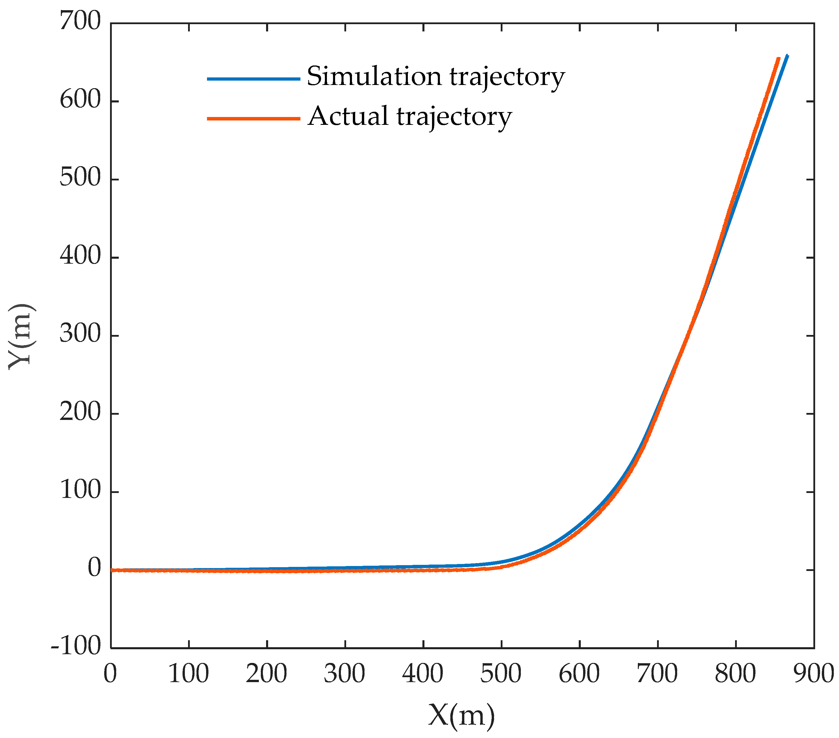
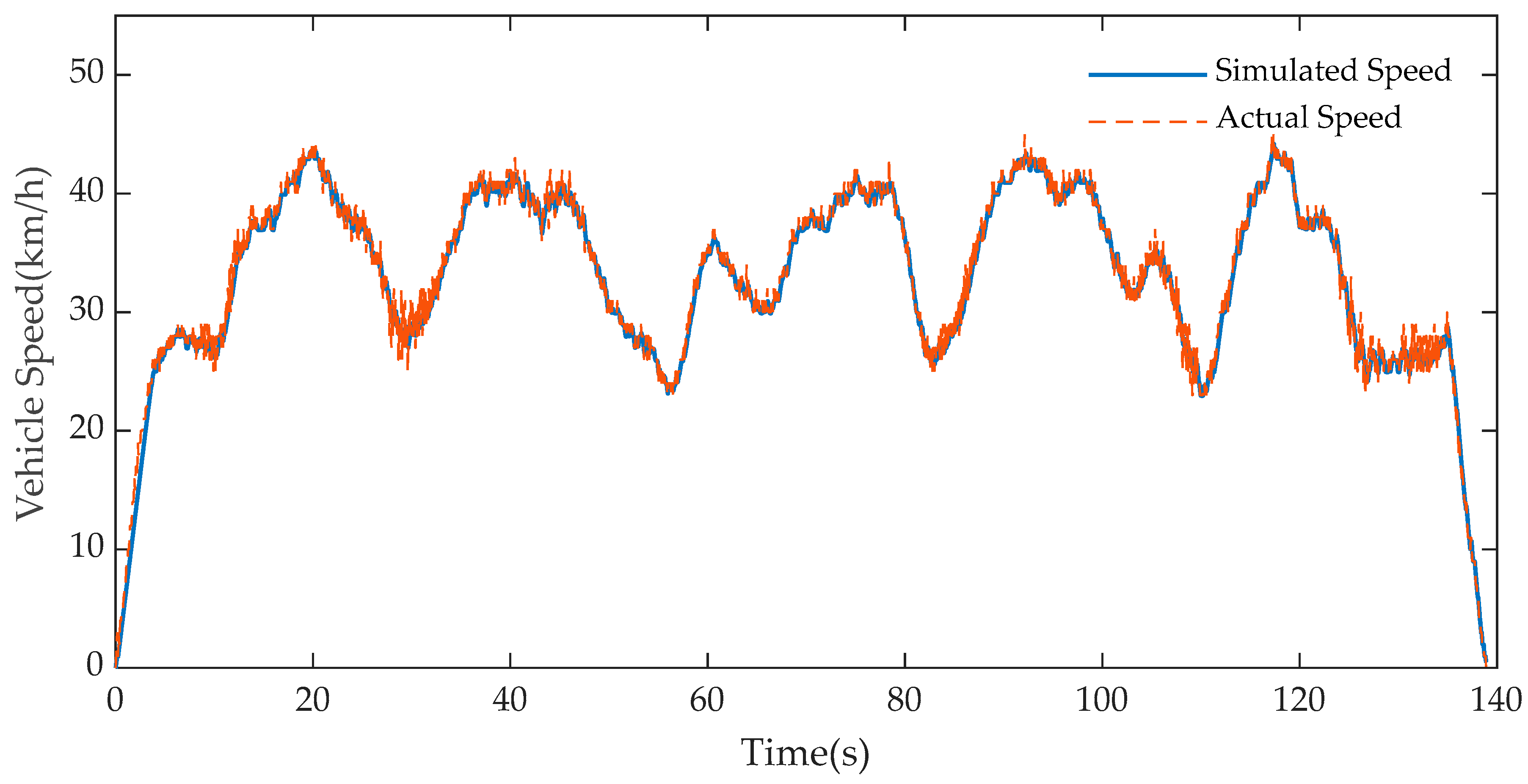
2.3. Verification of the Dynamics Model of Tracked Vehicles

Figure 4 and Figure 5 respectively present the comparison diagrams of the actual and simulation results of the driving trajectory and vehicle speed of a certain type of crawler vehicle on the dirt road. The vehicle weighs 24 tons, with $L$ being 4.4 m and $B$ being 2.71 m. In the simulation environment, $\mu$ is 0.8, $K$ is 0.015, and $f$ is 0.06. It is observable from the simulation results that this dynamic model can relatively accurately describe the state of the vehicle.

Figure 4. Vehicle trajectory comparison diagram.

Figure 5. Vehicle speed comparison diagram.

3. Construction of the MPC Controller

3.1. Construction of the Controller

The MPC controller utilizes the kinematic model to predict the vehicle’s position and posture within a future period, solves the optimal control sequence through quadratic programming, and outputs the first set of control quantities. During the process of quadratic programming solution, constraint conditions such as control increment limitations and control quantity magnitude limitations can be added, thereby considering the response capabilities of the actuators. The kinematic model of the tracked vehicle is a nonlinear equation and can be expressed as:

$$\dot{\mathit{X}}=f(\mathit{X},\mathit{u})$$

(11)

where the state quantities are $\mathit{X}={[X,Y,\theta ]}_T$, and the control quantities are $\mathit{u}={[v_s^l,v_s^r]}_T$.

Linearize and discretize Equation (4). Perform the Taylor expansion of the kinematic equation at the reference trajectory point and discretize it through the forward Euler method as follows:

$$\tilde{\mathit{X}}(k+1)=\mathit{A}\tilde{\mathit{X}}(k)+\mathit{B}\tilde{\mathit{u}}(k)$$

(12)

where $T_s$ is the sampling time, $v_{sd}^l,v_{sd}^r$ and are the reference values of the rotational speeds of the left and right driving wheels, and ${\theta }_d$ is the reference value of the heading angle.

$$\mathit{A}=\left[\begin{array}{ccc}1\hfill & 0\hfill & T_s(-{\displaystyle \frac{y_l{v}_{sd}^r-y_r{v}_{sd}^l}{y_l-y_r}}\sin {\theta }_d-{\displaystyle \frac{v_{sd}^l-v_{sd}^r}{y_l-y_r}}{x}_c\cos {\theta }_d)\\ 0\hfill & 1\hfill & T_s({\displaystyle \frac{y_l{v}_{sd}^r-y_r{v}_{sd}^l}{y_l-y_r}}\cos {\theta }_d-{\displaystyle \frac{v_{sd}^l-v_{sd}^r}{y_l-y_r}}{x}_c\sin {\theta }_d)\\ 0\hfill & 0\hfill & 1\end{array}\right]$$

$$\mathit{B}=\left[\begin{array}{cc}{T}_s(-{\displaystyle \frac{y_r}{y_l-y_r}}\cos {\theta }_d-{\displaystyle \frac{x_c}{y_l-y_r}}\sin {\theta }_d)& T_s({\displaystyle \frac{y_l}{y_l-y_r}}\cos {\theta }_d+{\displaystyle \frac{x_c}{y_l-y_r}}\sin {\theta }_d)\\ T_s(-{\displaystyle \frac{y_r}{y_l-y_r}}\sin {\theta }_d+{\displaystyle \frac{x_c}{y_l-y_r}}\cos {\theta }_d)& T_s({\displaystyle \frac{y_l}{y_l-y_r}}\sin {\theta }_d-{\displaystyle \frac{x_c}{y_l-y_r}}\cos {\theta }_d)\\ -{\displaystyle \frac{T_s}{y_l-y_r}}& {\displaystyle \frac{T_s}{y_l-y_r}}\end{array}\right]$$

Considering the need to limit the acceleration of the winding speed, let:

$$\mathit{\xi }(k)=\left[\begin{array}{c}\tilde{\mathit{X}}(k)\\ \tilde{\mathit{u}}(k-1)\end{array}\right]$$

(13)

The new state-space expression is:

$$\begin{array}{l}\mathit{\xi }(k+1)=\tilde{\mathit{A}}\mathit{\xi }(k)+\tilde{\mathit{B}}\Delta \mathit{U}(k)\\ \mathit{\eta }(k)=\tilde{\mathit{C}}\mathit{\xi }(k+1)\end{array}$$

(14)

where $\tilde{\mathit{A}}=\left[\begin{array}{cc}\mathit{A}& \mathit{B}\\ 0_{m\times n}& {\mathit{I}}_m\end{array}\right];\tilde{\mathit{B}}=\left[\begin{array}{c}\mathit{B}\\ {\mathit{I}}_m\end{array}\right];$ $n$ is the dimension of the state quantity; and $m$ is the dimension of the control quantity.

Through iterative derivation, the predicted output expression of the system can be obtained:

$$\mathit{Y}(k)=\mathit{\psi }\mathit{\xi }(k)+\mathit{\Theta }\Delta U(k)$$

(15)

The objective function of the model predictive controller is as follows:

$$\mathit{J}(k)={{\displaystyle \sum _{i=1}^{N_p}‖\mathit{\eta }(k+i\left|t\right.)-{\mathit{\eta }}_{ref}(k+i\left|t\right.)‖}}_Q^2+{{\displaystyle \sum _{i=1}^{N_c-1}‖\Delta \mathit{U}(k+i\left|t\right.)‖}}_R^2+\rho {\epsilon }^2$$

(16)

where $N_p$ is the prediction horizon; $N_c$ is the control horizon; $\rho$ is the weighting coefficient; and $\epsilon$ is the relaxation factor.

Transform it into the form of a quadratic form:

$$\mathit{J}=\left[\begin{array}{cc}\Delta {\mathit{U}}_T& \epsilon \end{array}\right]\left[\begin{array}{cc}{\mathit{\Theta }}_T\mathit{Q}\mathit{\Theta }& 0\\ 0& \rho \end{array}\right]\left[\begin{array}{c}\Delta \mathit{U}\\ \epsilon \end{array}\right]+\left[\begin{array}{cc}2{\mathit{E}}_T\mathit{Q}\mathit{\Theta }& 0\end{array}\right]\left[\begin{array}{c}\Delta \mathit{U}\\ \epsilon \end{array}\right]$$

(17)

The interior point method is adopted to solve it to obtain the control sequence, and the first group of control quantities is taken as the output of the controller.

3.2. Constraint Conditions

Considering the limited response capability of the motor and to prevent the vehicle from rollover, the increment of the rotational speed of the driving wheels is restricted, as well as the maximum value and the rotational speed difference between the left and right driving wheels.

The resistance received by the motor can be observed through the Luenberger observer. At the same time, according to the external characteristic curve of the motor, the maximum torque that the motor can output at the current rotational speed can be obtained, and the maximum rotational speed increment of the motors on both sides can be obtained:

$$\begin{array}{l}\Delta {\omega }_{\max }^l={\displaystyle \frac{\left(T_{e\max }^l-T_f^l\right)}{I_c}}\\ \Delta {\omega }_{\max }^r={\displaystyle \frac{\left(T_{e\max }^r-T_f^r\right)}{I_c}}\end{array}$$

(18)

where $I_c$ is the moment of inertia of the entire vehicle mass equivalent to the rotation of the motor

The maximum rotational speed increment of the driving wheel is obtained through the coupling mechanism and the reducer:

$$\left[\begin{array}{c}\Delta v_{s\max }^l\\ \Delta v_{s\max }^r\end{array}\right]={\displaystyle \frac{r}{i_b}}\left[\begin{array}{cc}{\displaystyle \frac{2+k}{2(1+k)}}& {\displaystyle \frac{k}{2(1+k)}}\\ {\displaystyle \frac{k}{2(1+k)}}& {\displaystyle \frac{2+k}{2(1+k)}}\end{array}\right]\left[\begin{array}{c}\Delta {\omega }_{\max }^l\\ \Delta {\omega }_{\max }^r\end{array}\right]$$

(19)

where $k$ is the planetary row parameter of the coupling mechanism, $i_b$ is the total reduction ratio, and $r$ is the radius of the driving wheel.

Bring it into the following formula as a constraint condition:

$$\begin{array}{l}\Delta {\mathit{u}}_{\min }(t+k)\le \Delta \mathit{u}(t+k)\le \Delta {\mathit{u}}_{\max }(t+k),\\ k=0,1,\cdots ,N_c-1\end{array}$$

(20)

The maximum rotational speed and the rotational speed difference of the driving wheel are restricted; that is, it is ensured that in the model prediction process, the control quantity of each prediction solution is within the constraint conditions. The maximum rotational speed can be obtained through the following formula:

$${\omega }_{\max }={\displaystyle \frac{P_{\max }}{\left(T_e^l+T_e^r\right)}}$$

(21)

Similarly, through the coupling mechanism, bring it into the following constraint conditions:

$$\left[\begin{array}{cc}{\mathit{A}}_t& 0\\ -{\mathit{A}}_t& 0\\ {\mathit{A}}_{wt}& 0\\ -{\mathit{A}}_{wt}& 0\end{array}\right]\left[\begin{array}{c}\Delta \mathit{U}\\ 0\\ \Delta \mathit{U}\\ 0\end{array}\right]\le \left[\begin{array}{c}{\mathit{U}}_{max}-{\mathit{U}}_t\\ -{\mathit{U}}_{max}+{\mathit{U}}_t\\ {\mathit{U}}_{wmax}-{\mathit{U}}_{wt}\\ -{\mathit{U}}_{wmax}+{\mathit{U}}_{wt}\end{array}\right]$$

(22)

where:

$$\begin{array}{cc}& {\mathit{A}}_t={\left[\begin{array}{cccc}1& 0& \cdots & 0\\ 1& 1& \cdots & 0\\ ⋮& ⋮& \ddots & 0\\ 1& 1& 1& 1\end{array}\right]}_{N_c\times N_c}\otimes {\mathit{I}}_m\hfill \\ & {\mathit{A}}_{wt}=\left[\begin{array}{cc}1& -1\\ 1& -1\end{array}\right]\otimes {\mathit{I}}_{N_c}\hfill \\ & {\mathit{U}}_t=1_{N_c\times 1}\otimes \mathit{u}(k-1)\hfill \\ & {\mathit{U}}_t=1_{N_c\times 1}\otimes \left[\begin{array}{c}{u}_1(k-1)-u_2(k-1)\\ u_1(k-1)-u_2(k-1)\end{array}\right]\hfill \end{array}$$

This constraint condition can simultaneously constrain the rotational speed value and the rotational speed difference on the left and right sides. Among them, $m$ is the dimension of the control quantity, and $\otimes$ represents the Kronecker product. $\mathit{u}(k-1)$ is the control quantity at the previous moment, and $u_1(k-1)$$u_2(k-1)$ represent the first and second elements in the control quantity, namely the rotational speeds of the left and right wheels. ${\mathit{U}}_{max},{\mathit{U}}_{wmax}$ are the maximum rotational speed of the driving wheel and the maximum rotational speed difference between the left and right driving wheels, respectively.

4. Construction of the TD3 Agent Compensation Module

4.1. Design of State Space and Action Space

In this paper, the TD3 agent is adopted to compensate for the deviations in vehicle position and attitude caused by the inaccuracy of the MPC controller model. Firstly, the lateral deviation, longitudinal deviation, and heading angle deviation of the vehicle in the global coordinate system need to be observed, which are $e_X,e_Y,e_{\theta }$, respectively. At the same time, the situation where the input states are the same but the expected actions are different should be avoided as much as possible to avoid the non-convergence of the model. The change rates of yaw rate, lateral deviation, longitudinal deviation, and heading angle deviation of the vehicle need to be introduced, which are ${\omega }_z,{\dot{e}}_X,{\dot{e}}_Y,{\dot{e}}_{\theta }$, respectively. Finally, considering the deviation between the trajectory predicted by the model and the actual trajectory, the deviations of the vehicle state at the current moment predicted by the vehicle state at the previous moment and the actual vehicle state at the current moment are introduced, which are ${\dot{e}}_{Xp},{\dot{e}}_{Yp},{\dot{e}}_{\theta p}$, respectively.

To sum up, the state space is designed as $s=[e_X,e_Y,e_{\theta },{\omega }_z,{\dot{e}}_X,{\dot{e}}_Y,{\dot{e}}_{\theta },{\dot{e}}_{Xp},{\dot{e}}_{Yp},{\dot{e}}_{\theta p}]$, and the action space is designed as the compensation amount $a=v_{\omega }$ for the speed difference of the left and right driving wheels.

4.2. Reward Function Design

The smaller the deviation of the vehicle’s position and attitude, the greater the reward value should be. In order to unify the magnitude of lateral deviation, longitudinal deviation, and yaw angle deviation, and to accelerate the convergence speed of the neural network, we set the deviation as an exponential function:

$$\begin{array}{l}{r}_{XY}=3e^{-0.05e_X^2-0.05e_Y^2}\\ r_{\theta }=0.3e^{-40e_{\theta }^2}\end{array}$$

(23)

In order to keep the output compensation rotational speed increment of the agent within the constraint range and prevent the instability of the tracked vehicle caused by the sudden change in its output, when the variation in the neural network output is too large, a certain penalty should be given. The penalty is designed as a continuous value to avoid the problem of non-convergence of training caused by giving different rewards for the same state:

$$r_{\dot{u}}=-0.5\left|a(k)-a(k-1)\right|$$

(24)

The final reward function is designed as

$$\left\{\begin{array}{l}r=r_{XY}+r_{\theta }+r_u\\ r_{XY}=3e^{-0.05e_X^2-0.05e_Y^2}\\ r_{\theta }=0.3e^{-40e_{\theta }^2}\\ r_{\dot{u}}=-0.5\left|a(k)-a(k-1)\right|\end{array}\right.$$

(25)

4.3. Design of the TD3 Agent

The TD3 algorithm improves the DDPG algorithm in three aspects. Introducing dual Critic networks to alleviate the overestimation problem; adding random noise to the target action; delaying the update of the Actor network.

First of all, the TD3 algorithm introduces dual Critic networks to alleviate the overestimation problem. The DDPG algorithm adopts the Actor–Critic structure, in which the Critic network uses the Double Q-learning (DQN) algorithm. Therefore, the DDPG algorithm will have the same overestimation problem as the DQN algorithm. The neural network update process of DQN can be expressed as:

$$\begin{array}{l}y=r+\gamma \cdot \underset{a}{\max }Q\left(s^{\prime },a^{\prime };w\right)\\ w\leftarrow w-\alpha \cdot \left[y-Q\left(s,a;w\right)\right]\cdot {\displaystyle \frac{\mathsf{\partial }Q\left(s,a;w\right)}{\mathsf{\partial }w}}\end{array}$$

(26)

In the formula, $y$ represents the target Q-value, $r$ is the reward of the environment, $\gamma$ is the discount factor that determines the priority of short-term rewards, $\alpha$ is the learning rate, $Q\left(s,a;w\right)$ represents the Q-value estimated by the Critic network at the current moment, $s^{\prime },a^{\prime }$ represent the state space and action space at the next moment, and $Q\left(s^{\prime },a^{\prime };w\right)$ represents the Q-value estimated by the Critic network at the next moment.

The maximization of Q-values and bootstrapping lead to the overestimation problem of Q-values. The training process is based on the method of experience replay, randomly extracting quadruples for update. In this process, the originally low Q-values may be overestimated, resulting in incorrect policies and reducing the training efficiency. The Target Network algorithm and the Double DQN algorithm alleviate the overestimation problem of Q-values to a certain extent, but the overestimation problem of Q-values in the DQN algorithm and DDPG still exists. The TD3 algorithm uses dual Critic networks. When calculating the Q-value estimated for the future at the next moment, it outputs the smaller output value among the two Target Critic networks:

$$y=r+\gamma \underset{i=1,2}{\min }{Q^{\prime }}_i\left(s^{\prime },{\mu }^{\prime }\left(s^{\prime };\varphi \right);w_i^{{Q^{\prime }}_i}\right)$$

(27)

In the formula, ${\mu }^{\prime }\left(\cdots ;\varphi \right)$ represents the Target Actor network, $Q^{\prime }\left(\cdots ;w^{Q^{\prime }}\right)$ represents the Target Critic network, ${\mu }^{\prime }\left(s^{\prime };\varphi \right)$ represents the output action at the next moment, and ${Q^{\prime }}_i\left(s^{\prime },a^{\prime };w_i^{{Q^{\prime }}_i}\right)$ represents the Q-value estimated at the next moment using the Target Critic network.

Secondly, the TD3 algorithm adds random noise to the target action. Using a deterministic policy network as the Actor network, when the Critic network is updated, the learning goal using the deterministic policy is easily affected by the error of function approximation, thereby increasing the variance of the target. This induced variance can be reduced through regularization. Therefore, the TD3 algorithm adds random noise to the target action:

$$\begin{array}{l}y=r+\gamma Q^{\prime }\left(s^{\prime },{\mu }^{\prime }\left(s^{\prime };\varphi \right)+\epsilon ;w^{Q^{\prime }}\right)\\ \epsilon ~clip\left(N\left(0,\sigma \right),-c,c\right)\end{array}$$

(28)

Finally, TD3 adopts the method of delayed update of the Actor network, and updates the Actor network after the update of the Critic network is stable. This improves the stability of the Actor network update.

The complete control algorithm structure is shown in Figure 6. The parameter settings of the training process are shown in Table 1:

Figure 6. Schematic diagram of the MPC-TD3 control algorithm.

Table 1. Training parameters.

Hyperparameter	Value
The number of layers of the Actor network	2
The number of neurons in each layer of the Actor	256
The learning rate of the Critic network	0.001
The learning rate of the Actor network	0.0001
discount factor	0.99
The size of the experience replay buffer	128
The update interval of the target network	2

During the training process, the TD3 agent randomly samples a quadruple from the experience replay pool, which contains the current moment’s tracked vehicle’s position and other state information $s$, the action output by the Actor network $a$, the reward given by the environment $r$, and the next moment’s state information $s^{\prime }$. The agent inputs $\left(s,a\right)$ into the Critic network to calculate the estimated Q-value at the current moment $Q_1,Q_2$. At the same time, it inputs the next moment’s state $s^{\prime }$ and action value ${\mu }^{\prime }\left(s^{\prime };\varphi \right)+\epsilon$ into the Target Critic network to calculate the estimated Q-value at the next moment ${Q^{\prime }}_1,{Q^{\prime }}_2$. Then, it takes the smaller of the two and adds it to the reward value to obtain the actual Q-value at the current moment. It separately calculates the TD error for each of the two Critic networks. Finally, it uses gradient descent to update the Critic network, and updates the Actor network using gradient ascent after the Critic network has been updated several times. The target network is updated using a soft update method.

During the online reasoning process, only the Actor network participates in the calculation. The agent calculates the compensation value in real time based on the current state information of the tracked vehicle.

5. Simulation and Analysis

5.1. Simulation Experiment

This article uses the dynamics model of a tracked vehicle built by MATLAB Simulink as the environment. The RL Agent module in the Simulink toolbox can be used for the training of agents, but the models trained thereby are difficult to deploy on the Huawei Atlas 200 DK controller. In this article, the Python language is used to write the MPC algorithm and train and infer the agent. Regarding the interaction problem between the agent and the environment, C code is generated by Simulink and then encapsulated as a DLL file to achieve the interaction between the agent and the controller in Python and the environment. As shown in Figure 7:

Figure 7. Simulation Experiment Data Interaction Diagram.

We validate the control effect using three trajectory conditions: straight-line, circular, and double-lane-change trajectory. The straight-line and circular trajectories can verify the vehicle’s track-following control effect under a constant desired turning radius. The double-lane-change trajectory is a variable-curvature trajectory, similar to actual driving scenarios such as overtaking and evading obstacles. It can verify the track-following control effect under this condition.

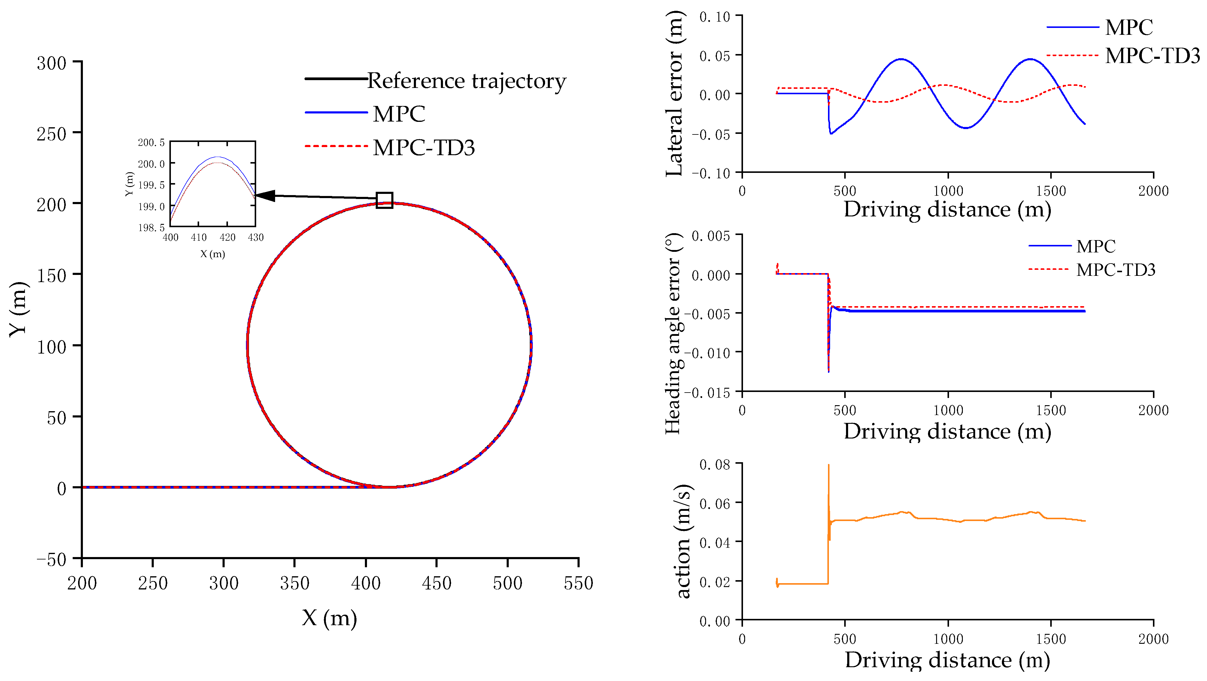
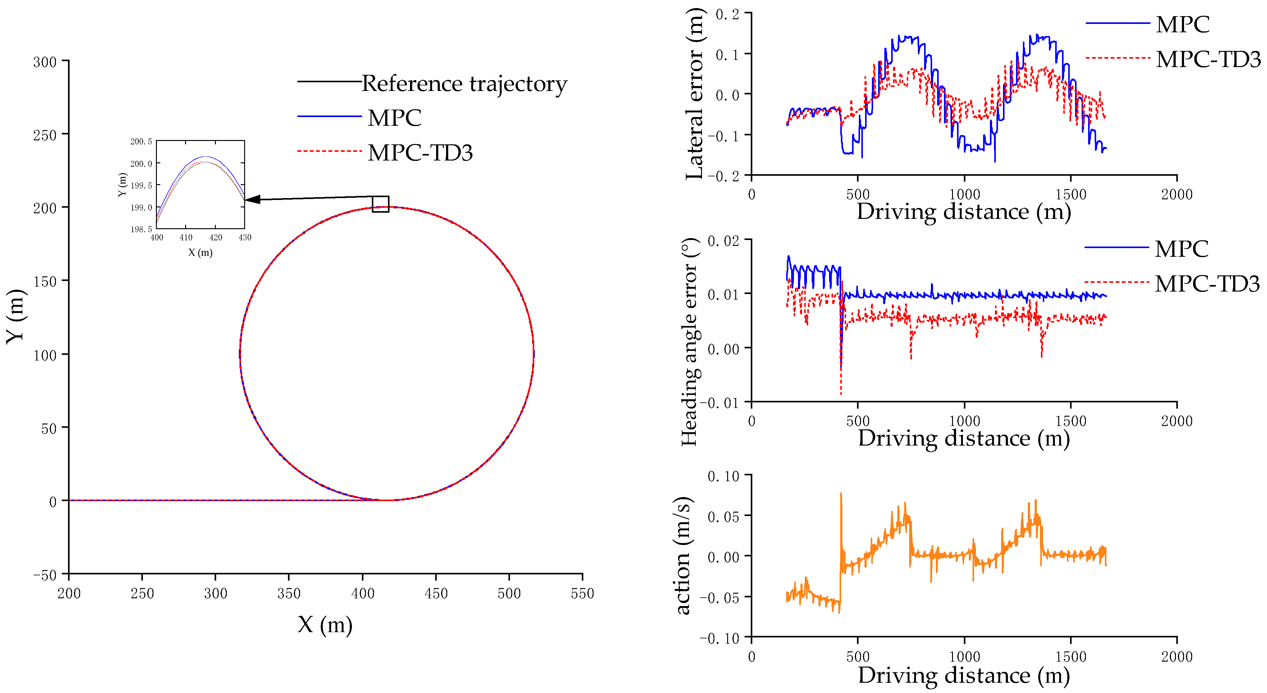
5.1.1. Straight-Line and Circular Trajectory Conditions in Simulation

Under this trajectory condition, the expected vehicle speed is set to 30 km/h. After driving in a straight line for 50 s, it tracks a circular path with a radius of 100 m. The simulation results are shown in Figure 8.

Figure 8. Simulation diagrams of straight-line and circular trajectory conditions.

From the simulation results, it can be concluded that under the trajectory conditions of straight lines and circular trajectories, compared with the MPC controller, the mean values of the lateral deviation and the heading angle deviation of the MPC-TD3 controller proposed in this paper have decreased by 58.18% and 10.27% respectively. Moreover, it can be seen that the penalty for the output deviation value in the reward function has achieved a very good effect. The output value of the agent has no sudden change and has better stability.

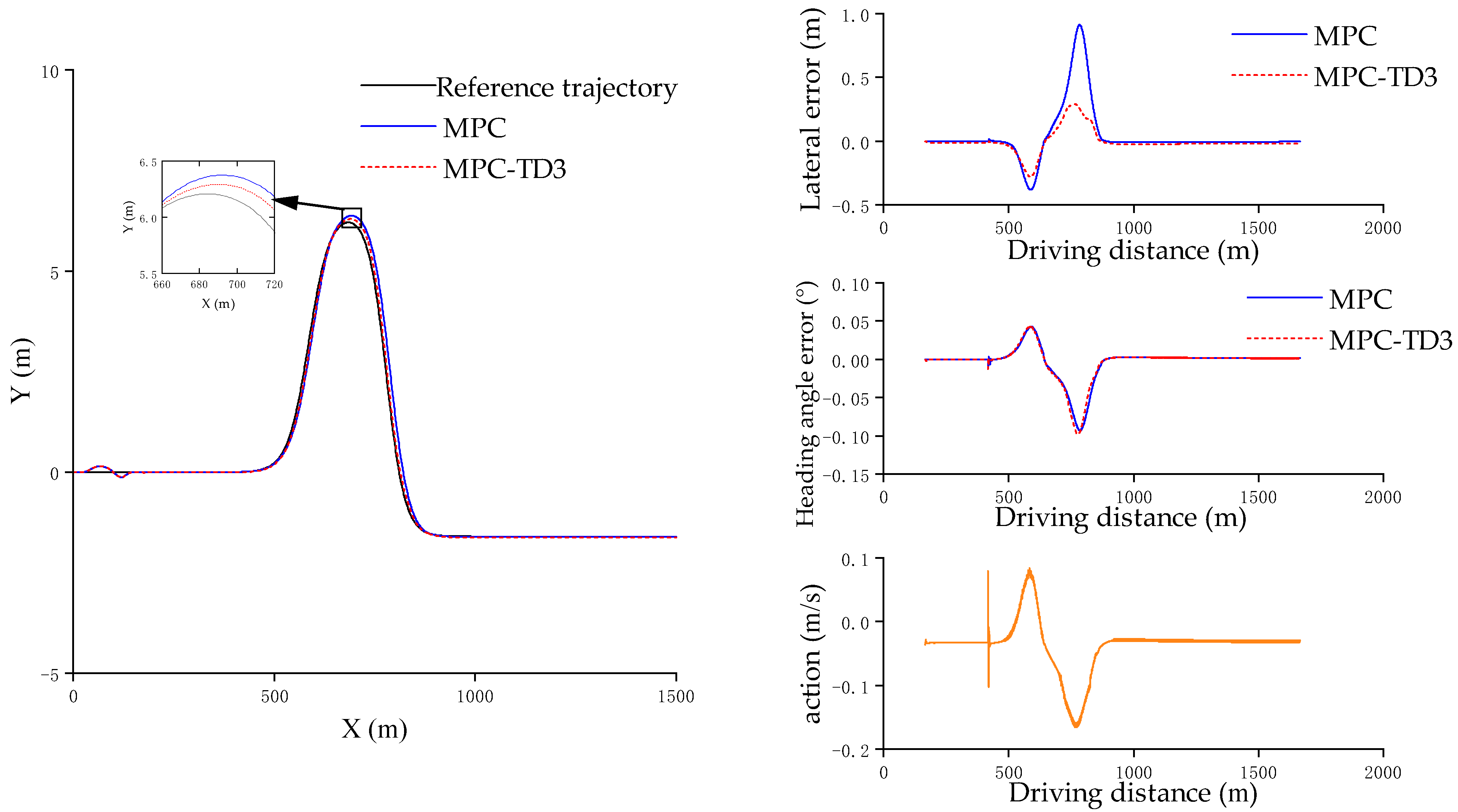
5.1.2. Double-Lane-Change Trajectory Conditions

Under this trajectory condition, the expected vehicle speed is set at 30 km/h. After a period of linear acceleration, it enters the double-lane-change path. The simulation results are shown in Figure 9.

Figure 9. Simulation diagrams of double-lane-change trajectory conditions.

It can be obtained from the simulation results that under the double-lane-change trajectory condition, the maximum lateral deviation has decreased from 0.91 m to 0.29 m, reducing by 68.13%. The mean values of the lateral deviation and the heading angle deviation have decreased by 34.10% and 0.18%, respectively.

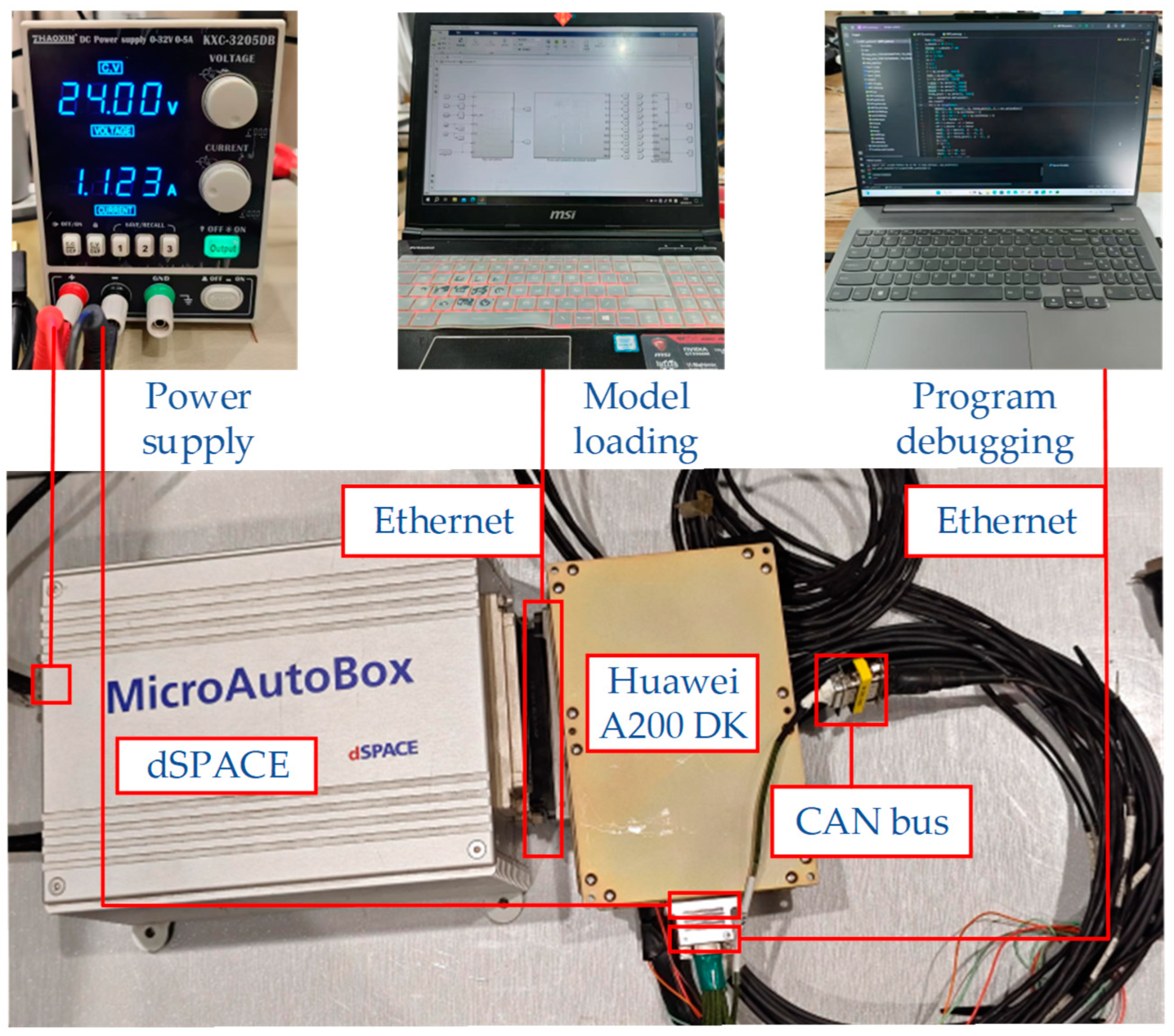
5.2. Hardware-in-the-Loop Experiment and Analysis

The hardware-in-the-loop simulation experiment is shown in Figure 10. The MPC-TD3 algorithm is deployed on the Atlas 200 DK development board produced by Huawei in Shenzhen, China, which adopts the CANN architecture. It is necessary to convert the agent saved by Pytorch into the OM model and deploy it on the development board, and conduct online reasoning using the AscendCL toolchain. The simulation environment runs in dSPACE, and the CAN bus is used for communication between the controller and dSPACE.

Figure 10. Hardware-in-the-Loop Experimental System.

5.2.1. Straight-Line and Circular Trajectory Conditions in Hardware-in-the-Loop Experiment

It can be seen from Figure 11 that under this working condition with the vehicle speed of 30 km/h, when comparing the MPC-TD3 controller with the MPC controller, the mean values of the lateral deviation and the heading angle deviation have decreased by 41.67% and 37.51%, respectively. The output of the agent, due to communication interference and noise, fluctuates more than that in the simulation case, but it is still within the controllable range.

Figure 11. Hardware-in-the-Loop simulation diagrams of straight-line and circular trajectory conditions.

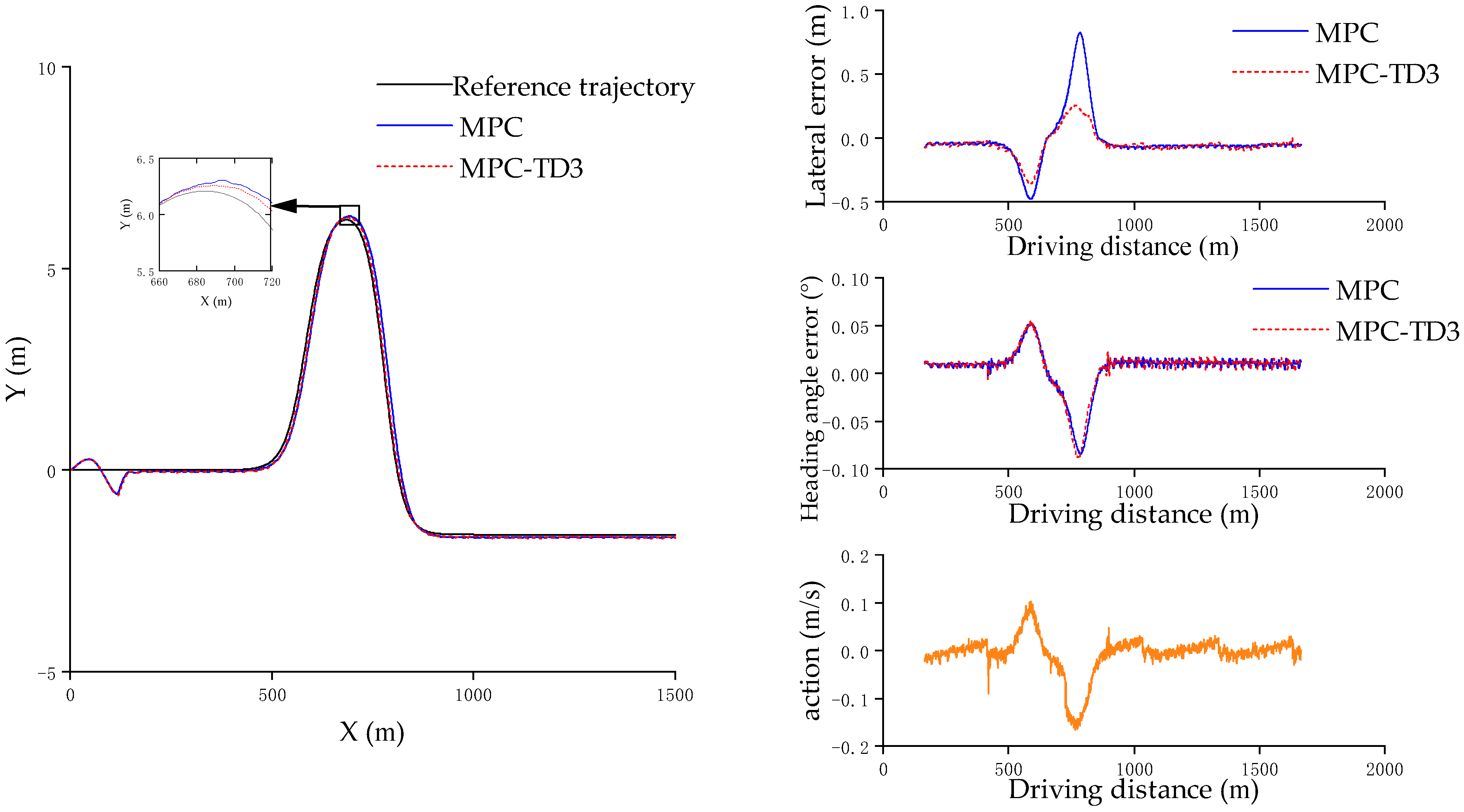
5.2.2. Double-Lane-Change Trajectory Conditions in Hardware-in-the-Loop Experiment

It can be seen from Figure 12 that under this trajectory condition with the vehicle speed of 30 km/h, when comparing the MPC-TD3 controller with the MPC controller, the maximum lateral deviation has decreased from 0.82 m to 0.36 m, a reduction of 56.10%. The mean value of the lateral deviation has decreased by 22.55%. It can be seen that the average calculation time of the MPC algorithm is 0.0448 s, and the average calculation time of the TD3 algorithm is 0.0008 s. The addition of the TD3 algorithm has almost no impact on the solution time.

Figure 12. Hardware-in-the-Loop simulation diagrams of double-lane-change trajectory conditions.

6. Future Research Directions

The safety of tracked vehicle trajectory tracking control is of great importance. In this paper, the intelligent agent is constrained by using a penalty surrogate variable method, thus achieving vehicle stability. However, it is inevitable that the intelligent agent will output abrupt changes during the initial training. How to increase the exploratory nature of the intelligent agent’s training while ensuring safety is a very worthy research direction. In future research, we will try to combine human experience with the training of intelligent agents, and at the same time, impose safety constraints during training to enhance the safety of the training.

7. Results

In this paper, aiming at the problem of insufficient trajectory tracking accuracy of tracked vehicles under different trajectory conditions, an MPC-TD3 controller is proposed by combining the model-based and data-based methods, achieving an improvement in trajectory tracking accuracy. The following conclusions are obtained through simulation experiments and hardware-in-the-loop experiments: (1) The TD3 algorithm is used to adaptively compensate the output of the MPC controller, making up for the insufficient trajectory tracking accuracy caused by inaccurate vehicle models and environmental interferences, and achieving an improvement in trajectory tracking accuracy. (2) The designed reward function not only improves the control accuracy but also suppresses the problems of vehicle instability caused by the output mutation of the TD3 agent and the non-convergence of training. (3) The experimental verification under circular trajectory conditions and double-lane-change trajectory conditions is completed. Compared with the traditional MPC algorithm, the algorithm proposed in this paper reduces the lateral error by 41.67% and 22.55%, respectively, verifying the effectiveness of the algorithm.

References

- Wang, J.; Gao, S.; Wang, K.; Wang, Y.; Wang, Q. Wheel torque distribution optimization of four-wheel independent-drive electric vehicle for energy efficient driving. Control Eng. Pract. 2021, 110, 104779. [Google Scholar] [CrossRef]
- Husain, I.; Ozpineci, B.; Islam, M.S.; Gurpinar, E.; Su, G.J.; Yu, W.; Chowdhury, S.; Xue, L.; Rahman, D.; Sahu, R.; et al. Electric drive technology trends, challenges, and opportunities for future electric vehicles. Proc. IEEE 2021, 109, 1039–1059. [Google Scholar] [CrossRef]
- Yuan, Y.; Gai, J.; Zeng, G.; Zhou, G.; Li, X.; Ma, C. Analysis and Experimental Verification of Yaw Motion Response Characteristics of High-speed Tracked Vehicle. Acta Armamentarii 2024, 45, 1094–1107. [Google Scholar]
- Yuan, Y.; Gai, J.; Zhou, G.; Gao, X.; Li, X.; Ma, C. Analysis of High-Speed Electric Tracked Vehicle’s Handling Characteristics. Acta Armamentarii 2023, 44, 203–213. [Google Scholar]
- Hou, X.; Ma Yue Xiang, C. Research on Steering Stability Control of Electric Drive Tracked Vehicle. J. Mech. Eng. 2024, 60, 233–244. [Google Scholar]
- Zhang, J.; Wang, H.; Zheng, J.; Cao, Z.; Man, Z.; Yu, M.; Chen, L. Adaptive sliding mode-based lateral stability control of steer-by-wire vehicles with experimental validations. IEEE Trans. Veh. Technol. 2020, 69, 9589–9600. [Google Scholar] [CrossRef]
- Sun, W.; Wang, S. A Review of the Technical Content of Autonomous Vehicle. Int. J. Syst. Eng. 2018, 2, 42–46. [Google Scholar]
- AbdElmoniem, A.; Osama, A.; Abdelaziz, M.; Maged, S.A. Accurate path tracking by adjusting look-ahead point in pure pursuit method. Int. J. Automot. Technol. 2021, 22, 119–129. [Google Scholar]
- AbdElmoniem, A.; Osama, A.; Abdelaziz, M.; Maged, S.A. A path-tracking algorithm using predictive Stanley lateral controller. Int. J. Adv. Robot. Syst. 2020, 17, 1729881420974852. [Google Scholar] [CrossRef]
- Farag, W. Complex trajectory tracking using PID control for autonomous driving. Int. J. Intell. Transp. Syst. Res. 2020, 18, 356–366. [Google Scholar] [CrossRef]
- Xu, L.; Du, J.; Song, B.; Cao, M. A combined backstepping and fractional-order PID controller to trajectory tracking of mobile robots. Syst. Sci. Control Eng. 2022, 10, 134–141. [Google Scholar] [CrossRef]
- Zhao, Z.; Liu, H.; Chen, H.; Hu, J.; Guo, H. Kinematics-aware model predictive control for autonomous high-speed tracked vehicles under the off-road conditions. Mech. Syst. Signal Process. 2019, 123, 333–350. [Google Scholar] [CrossRef]
- Srikonda, S.; Norris, W.R.; Nottage, D.; Soylemezoglu, A. Deep Reinforcement Learning for Autonomous Dynamic Skid Steer Vehicle Trajectory Tracking. Robotics 2022, 11, 95. [Google Scholar] [CrossRef]
- Liu, M.; Zhao, F.; Yin, J.; Niu, J.; Liu, Y. Reinforcement-tracking: An effective trajectory tracking and navigation method for autonomous urban driving. IEEE Trans. Intell. Transp. Syst. 2021, 23, 6991–7007. [Google Scholar] [CrossRef]
- Shan, Y.; Zheng, B.; Chen, L.; Chen, L.; Chen, D. A reinforcement learning-based adaptive path tracking approach for autonomous driving. IEEE Trans. Veh. Technol. 2020, 69, 10581–10595. [Google Scholar] [CrossRef]
- Wang, S.; Yin, X.; Li, P.; Zhang, M.; Wang, X. Trajectory tracking control for mobile robots using reinforcement learning and PID. Iran. J. Sci. Technol. Trans. Electr. Eng. 2020, 44, 1059–1068. [Google Scholar] [CrossRef]
- Chen, I.M.; Chan, C.Y. Deep reinforcement learning based path tracking controller for autonomous vehicle. Proc. Inst. Mech. Eng. Part D J. Automob. Eng. 2021, 235, 541–551. [Google Scholar] [CrossRef]
- Sabiha, A.D.; Kamel, M.A.; Said, E.; Hussein, W.M. ROS-based trajectory tracking control for autonomous tracked vehicle using optimized backstepping and sliding mode control. Robot. Auton. Syst. 2022, 152, 104058. [Google Scholar] [CrossRef]
- Ruslan, N.A.I.; Amer, N.H.; Hudha, K.; Kadir, Z.A.; Ishak SA, F.M.; Dardin, S.M.F.S. Modelling and control strategies in path tracking control for autonomous tracked vehicles: A review of state of the art and challenges. J. Terramech. 2023, 105, 67–79. [Google Scholar] [CrossRef]
- Al-Jarrah, A.; Salah, M. Trajectory tracking control of tracked vehicles considering nonlinearities due to slipping while skid-steering. Syst. Sci. Control Eng. 2022, 10, 887–898. [Google Scholar] [CrossRef]
Disclaimer/Publisher’s Note: The statements, opinions and data contained in all publications are solely those of the individual author(s) and contributor(s) and not of MDPI and/or the editor(s). MDPI and/or the editor(s) disclaim responsibility for any injury to people or property resulting from any ideas, methods, instructions or products referred to in the content. |
© 2024 by the authors. Licensee MDPI, Basel, Switzerland. This article is an open access article distributed under the terms and conditions of the Creative Commons Attribution (CC BY) license (https://creativecommons.org/licenses/by/4.0/).