Article

Hardware-in-the-Loop Simulation of Flywheel Energy Storage Systems for Power Control in Wind Farms

1
Intelligent Control Institute, Hunan Railway Professional Technology College, Zhuzhou 412001, China
2
National Engineering Research Center for Robot Vision Perception and Control, College of Electrical and Information Engineering, Hunan University, Changsha 410082, China
*
Author to whom correspondence should be addressed.
Electronics 2024, 13(18), 3610; https://doi.org/10.3390/electronics13183610
Submission received: 25 August 2024 / Revised: 8 September 2024 / Accepted: 9 September 2024 / Published: 11 September 2024

Abstract

:
Flywheel energy storage systems (FESSs) are widely used for power regulation in wind farms as they can balance the wind farms’ output power and improve the wind power grid connection rate. Due to the complex environment of wind farms, it is costly and time-consuming to repeatedly debug the system on-site. To save research costs and shorten research cycles, a hardware-in-the-loop (HIL) testing system was built to provide a convenient testing environment for the research of FESSs on wind farms. The focus of this study is the construction of mathematical models in the HIL testing system. Firstly, a mathematical model of the FESS main circuit is established using a hierarchical method. Secondly, the principle of the permanent magnet synchronous motor (PMSM) is analyzed, and a nonlinear dq mathematical model of the PMSM is established by referring to the relationship among d-axis inductance, q-axis inductance, and permanent magnet flux change with respect to the motor’s current. Then, the power grid and wind farm test models are established. Finally, the established mathematical models are applied to the HIL testing system. The experimental results indicated that the HIL testing system can provide a convenient testing environment for the optimization of FESS control algorithms.

1. Introduction

Wind energy is a clean and pollution-free renewable energy source, and there is a substantial amount of wind energy. The use of wind energy for power generation is very environmentally friendly; therefore, it is increasingly receiving attention from the Chinese government. At the end of 2023, the installed capacity of wind power generation systems in China was 2919.65 million kilowatts, an increase of 13.9% compared to the end of the previous year [1]. The installed capacity of wind power connected to the power grid is 44.134 million kilowatts, an increase of 20.7% compared to the end of the previous year [1]. It can be observed that the installed capacity of wind power connected to the power grid is much lower than the installed capacity of power generation. Abandoning wind and limiting electricity is an important reason. A further reason is that the instability of wind energy results in fluctuations and intermittency in the output power of wind farms [2,3]. When the output power of wind farms cannot accommodate power grid connection conditions, the traditional approach is to abandon wind power and limit electricity, which results in substantial energy waste. Fortunately, the output power of wind farms can be balanced when using energy storage methods, and wind power abandonment and limitations to electricity can also be reduced. Chemical, electromagnetic, and mechanical energy storage methods are common [2]. Among them, FESSs are one of the most common mechanical energy storage methods, where electric energy is stored in a high-speed rotating flywheel rotor [3]. During the acceleration or deceleration of the flywheel rotor, electrical energy and mechanical energy are converted into one another [4,5]. The outstanding advantages of FESSs include long service life, low charging cost, and environmental friendliness. FESS is currently a popular method for regulating the power of wind farms. Due to the particularity and complexity of the operating environment, the on-site debugging of FESSs for wind farms is difficult [5,6]. Therefore, it is necessary to build a simulation testing environment in the laboratory so that the FESS algorithm can be repeatedly verified before on-site debugging. In this manner, the development cycle is shortened, and development costs are also saved.
In general, PCs are used for simulation testing systems. However, due to the difference between PC and actual hardware conditions, traditional simulation testing systems inevitably have some deviation from the actual system. HIL is a more advanced simulation test method that generally comprises a real-time simulator and a physical controller [5]. Among them, one part of the system runs in the real-time simulator via mathematical models, and the other parts still run within the physical controller [5]. Finally, the two parts are connected for debugging and experimentation. An HIL testing system reproduces the field conditions to the greatest extent in a laboratory environment; thus, the test results are closer to the field test results than traditional simulation test systems; this is more conducive to system optimization [5].
This article outlines the construction of an HIL testing system to assist in the optimization of the control algorithm of FESSs in wind farms. This study involves the realization of an FESS control algorithm, the construction of mathematical models, and the construction of an HIL testing system. Classic FESS control algorithms include field-oriented control, direct torque control, artificial intelligence control, etc. [6]. For example, the authors of [7] presented an energy management and control system designed with an integrated FESS for residential users. The power/current tracking of the machine-side and the network-side converter was the key to the proposed FESS control system. The authors of [8] presented a high-speed FESS for DC1500V transit transportation traction grids, and a three-level neutral point clamped control method for high-speed maglev permanent magnet motors based on square wave modulation–two-phase conduction was proposed. The authors of [9] presented an FESS controlled via a modeled predictive control algorithm for short-term high-frequency power smoothing in wind farms. The high-frequency components of a wind farm’s output power were extracted via a wavelet packet decomposition algorithm, and it was optimized using mathematical interpolation. The authors of [10] presented a new adaptive droop controller for FESSs in order to maximize the contribution of the FESS during the first instances following a frequency deviation. The droop coefficient was altered in real time according to the grid’s frequency. The authors of [11] presented 3D-SVPWM technology in order to operate a phase-loss PMSM in FESSs. A dual closed-loop control strategy relative to speed and current control was proposed.
The establishment of mathematical models is key to simulations, and the scholarly research provides references. For example, the authors of [12] presented nonlinear PMSM modeling and a traditional model reference adaptive system of FESSs. The authors of [13] presented linear frequency control modeling and a primary frequency modulation control model of FESS-assisted wind power. The authors of [5] presented models of dynamic flywheels and wind farms. The authors of [14] presented an HIL simulation of wind power, including mathematical models of wind farms, concentrated wind turbines, PMSMs, rectifiers, inverters, and batteries. The authors of [15] presented models of PMSMs, power compensation control strategies, and wind farms. Among these, the actual wind power output of a wind turbine was measured every minute, and 51-min variable data were used for the wind farm models. The authors of [16] presented six different numerical modeling methods for horizontal-axis wind turbine arrays in large wind farms. The authors of [17] presented effective windage loss modeling in FESSs. The proposed model was based on several analytical and semi-empirical windage loss solutions for cylindrical and planar surface interactions.
The HIL testing system can provide convenient simulation conditions for algorithm optimization. For example, the authors of [18] presented an HIL testing system to verify the correctness of the proposed fault-tolerant control strategy for offshore wind farms. The system consisted of a wind park computer simulator, interface circuits, and an onboard processor. The authors of [19] presented an HIL testing system for FESS-based microgrid controllers. Experiments were performed with real equipment, and the FESS was connected to a digital real-time simulator. Several frequency events were triggered, and the frequency profile was observed to compare the microgrid’s performance with and without the developed frequency control. The authors of [20] presented an HIL testing system to validate the performance of a proposed adaptive droop control strategy. The controller was simulated in real time via an Opal-RT OP5700 real-time simulator, and it was implemented on a real commercial 60 kW high-speed FESS. The simulation time steps only took 24 μs. The authors of [21] presented an HIL platform in an NI myRIO 1900 to evaluate the performance of control algorithms in a small wind system that serves as a distributed generator. The authors of [22] presented a wind tunnel HIL testing system to make up for the shortages of traditional HILs with respect to flight control system evaluation, and it further reduced the risks of flight tests. The authors of [23,24] presented a testing system in which converters and controllers were simulated using MATLAB 2018, and the models were simulated in the HIL testing platform.
This article is organized into seven sections. Section 1 comprises the introduction; Section 2 describes the structure of wind farms with FESSs; Section 3 describes the structure of HIL testing systems; Section 4 describes the modeling of FESSs, including the main circuit, PMSMs, and FESS dynamic models; Section 5 describes the modeling of wind farms and power grids; and Section 6 describes the experiments on HIL testing systems. Finally, Section 7 provides conclusions.

2. Structure of Wind Farms with FESSs

A structural diagram of wind farms with FESSs is shown in Figure 1. An FESS is mainly composed of a flywheel, a PMSM, a main circuit, a controller, etc. [3]. The main circuit is mainly composed of a motor-side inverter, a network-side inverter, and a filter circuit. The operation of FESSs is divided into three states: energy charging, energy discharging, and energy retention [2,3,4,5]. The energy charging state comprises the following: When the output power of the wind turbine is higher than the power grid, the energy is output from the network side to the motor side. The motor is an electric motor, the flywheel rotates rapidly, and electrical energy is converted into kinetic energy [5]. The 50 Hz alternating current (AC) is tuned to the rated frequency via the network-side and motor-side inverters in order to control the movement of the flywheel. The energy retention state comprises the following: When the flywheel’s speed approaches the limit, it no longer increases. The energy-discharging state is as follows: When the output power of the wind turbine is lower than the power grid, energy is outputted from the motor side to the network side. The motor is an engine, and kinetic energy is converted into electrical energy [5]. In this case, the output energy of the flywheel’s rotor is fed back to the power grid via the motor-side and network-side inverters. During the discharging process, the flywheel’s speed decreases continuously. When the preset minimum working speed is reached, the system stops releasing energy. The role of the controller is to run the FESS control algorithm. The total power of the power grid is the output power P d of the wind farm plus the output power P f of the FESS.

3. The Structure of HIL Testing Systems

According to the system structure described in Figure 1, an HIL testing system was built, as shown in Figure 2. The testing system consists of three parts: a PC, a real-time simulator, and a physical controller. Among these, the function of the PC is model building, testing, and downloading, in addition to the real-time monitoring of simulation processes. The function of the real-time simulator is to carry out real-time calculations of the models. This system uses a real-time simulator developed by the German dSPACE company. The dSPACE simulator is built based on CPU+FPGA architecture and high-speed IO technology [24]. Among them, FPGA is mainly used for the calculation of models with complex structures and high operation rates and to maintain calculation accuracy [24]. FPGA can greatly reduce the CPU’s calculation burden and improve the working efficiency of real-time simulators [24]. As shown in Figure 1, the flywheel dynamics model, PMSM model, main circuit model, power grid model, and other models in FESSs are run in the real-time simulator. Among these, the flywheel dynamics, the power grid, and wind farm models are run using the CPU board; the PMSM and main circuit models are run using the FPGA board. This article focuses on the construction of these mathematical models.
The function of the physical controller is to run the FESS control algorithm. The physical controller is actually the FESS controller shown in Figure 1. The control algorithm is divided into motor-side control algorithms and network-side control algorithms. The function of the motor-side control algorithm is to collect the angular velocity of PMSMs and the three-phase input stator current of PMSMs given the power and other signals sent by the real-time simulator, and it outputs PWM signals to drive the motor-side converter in order to control the rotation of the PMSM [5]. The function of the network-side control algorithm is to collect the three-phase voltage of the power grid and the three-phase current of network-side converters sent by the real-time simulator, and it outputs PWM signals to drive the network-side converter according to the given active and reactive power; finally, it compensates the output power of the wind farm [5]. The specific definitions of the parameters in Figure 2 are defined in the Nomenclature Section.

4. Modeling of FESSs

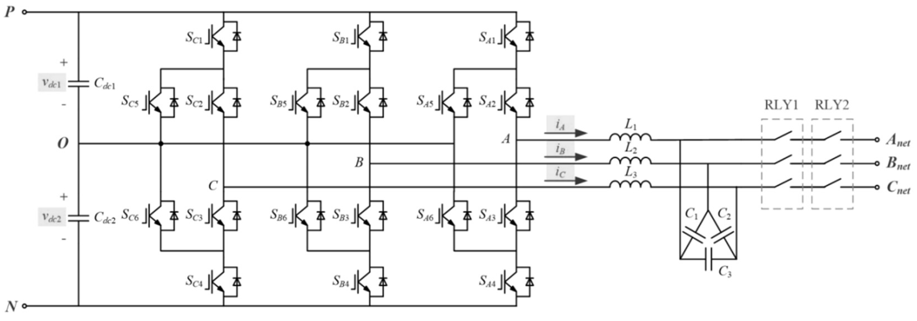
4.1. Modeling of the Main Circuit

As shown in Figure 2, the main circuit model includes a motor-side inverter, a DC bus circuit, a network-side inverter, a network-side filter, and a network-side transformer. The most critical part is the motor-side and network-side inverters. The circuit of the network-side inverter is shown in Figure 3. The structure of the motor-side inverter is basically the same as that of the network-side inverter; thus, the establishment of the motor-side inverter model is not discussed in this paper. As shown in Figure 3, S C 1 ~ S C 6 , S B 1 ~ S B 6 , and S A 1 ~ S A 6 are IGBT (insulated gate bipolar transistor) devices; C d c 1 and C d c 2 are DC support capacitors; L 1 , L 2 , and L 3 are AC filter inductors; C 1 , C 2 , and C 3 are AC filter capacitors. The main circuit model is divided into IGBT, inductor, capacitor, resistor, and other models via hierarchical modeling. The main circuit model of FESS is formed via superposition and a combination of each part’s model.

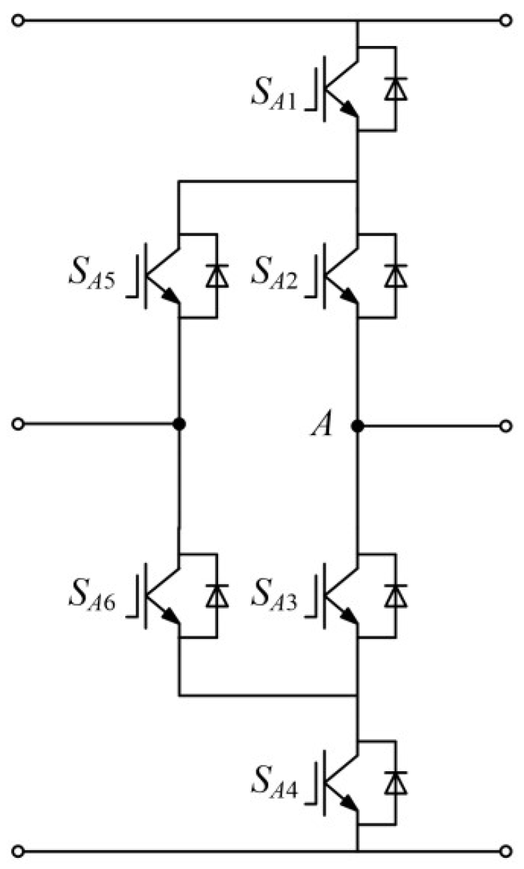
4.1.1. Modeling of ANPC Topology

As shown in Figure 3, the IGBTs in the circuit comprise three identical bridge arms A, B, and C, which form the active neutral point clamped (ANPC) topology. A single bridge arm consists of six IGBTs, as shown in Figure 4. The A-phase bridge arm is taken as an example to illustrate the modeling of ANPC topology. IGBTs in the inverter circuit are switching elements with operating states that vary at high frequencies. Smaller simulation steps are needed to reflect the dynamic characteristics, and the modeling method will affect overall accuracies and efficiencies in simulations. The common modeling methods of inverter circuits comprise detailed modeling, average modeling, adjoint network modeling, etc. Among these, the adjoint network modeling method is an innovative circuit analysis method, and it simplifies the transient analysis process of complex circuits by discretizing dynamic components and constructing adjoint networks. This method improves analysis efficiency and accuracy, and its models are easier to program.
Now, adjoint network modeling methods are used to model the A-phase bridge arm:
  • Step 1: Let the circuit time interval T (simulation step) be 1 × 10⁻⁸ s.
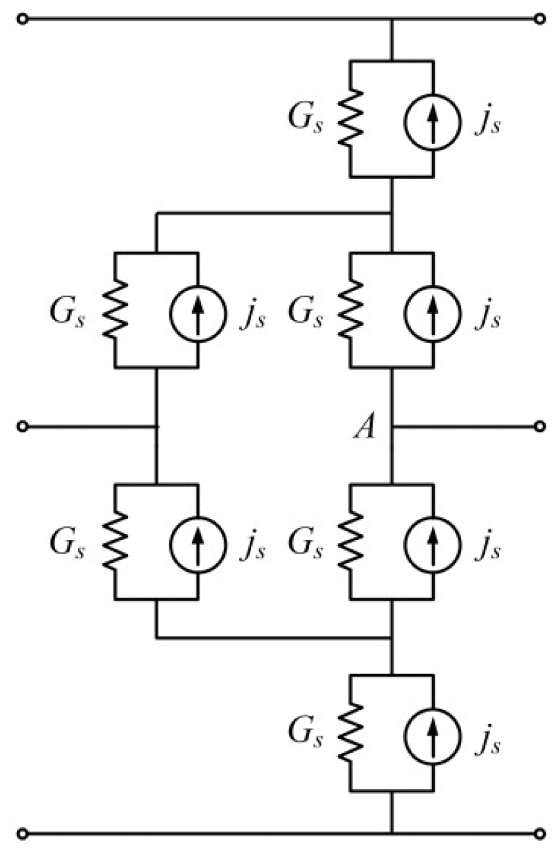
  • Step 2: At each time interval, a single IGBT is replaced with its discrete model.
The circuit of a single IGBT is shown in Figure 5a, where u s ( k + 1 ) represents the voltage at both ends of the IGBT at k + 1 simulation step. i s ( k + 1 ) represents the current flowing through the IGBT at the k + 1 simulation step. s is a Boolean quantity that indicates the IGBT’s switch status. IGBT is a fully controlled device with a switching state that is determined via an external control signal. Ideally, the relationship between s and u s ( k + 1 ) , i s ( k + 1 ) is shown in Equation (1).
o p e n : s ( k + 1 ) = 1 , u s ( k + 1 ) = 0 c l o s e : s ( k + 1 ) = 0 , i s ( k + 1 ) = 0
The IGBT is equivalent to a small inductor when it is switched on, and it is equivalent to a small capacitor when it is off. The mathematical discretization model of inductance is shown in Equation (2), and the mathematical discretization model of capacitance is shown in Equation (3). Here, T is the simulation step, G l is the admittance of the equivalent inductance, G c is the admittance of the equivalent capacitance, L s is the equivalent inductance, and C s is the equivalent capacitance. j l is the inductively equivalent current source, and j c is the capacitance equivalent current source.
i l ( k + 1 ) T L s u l ( k + 1 ) + i l ( k ) = G l u l ( k + 1 ) j l ( k + 1 )
i c ( k + 1 ) C s T u c ( k + 1 ) C s T u c ( k ) = G c u c ( k + 1 ) j c ( k + 1 )
  • Step 3: According to the discrete model, the adjoint network corresponding to the original circuit is constructed.
In Equations (2) and (3), let G s = G l = G c and j s ( k + 1 ) = j l ( k + 1 ) = j c ( k + 1 ) . Figure 5a is equivalent to the parallel connection of G s and j s , as shown in Figure 5b. G s denotes universal admittance, and j s denotes the controlled current source. The value of j s is shown in Equation (4). If G s remains a constant and j s changes according to Equation (4), the model of IGBT is obtained. In order to maintain the convergence of the system, G s is generally selected between 0 and 10.
j s ( k + 1 ) = i s ( k ) , ( o p e n : s ( k + 1 ) = 1 ) G s u s ( k ) , ( c l o s e : s ( k + 1 ) = 0 )
  • Step 4: According to the single IGBT equivalent circuit, the equivalent circuit of the A-phase bridge arm is obtained, as shown in Figure 6.

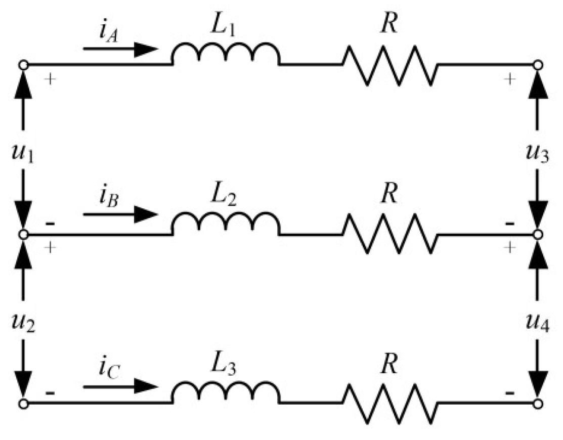
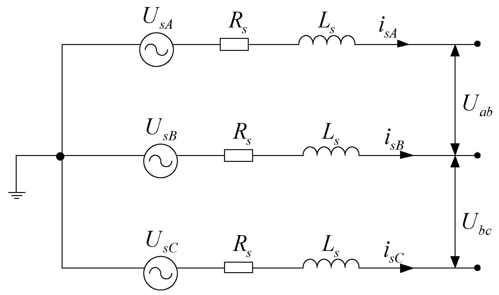
4.1.2. Modeling of Inductive Filter

As shown in Figure 3, the inductive filter consists of L 1 , L 2 , and L 3 . The equivalent circuit of the inductive filter is shown in Figure 7. i A denotes the current flowing through L 1 , i B denotes the current flowing through L 2 , i C denotes the current flowing through L 3 , and R denotes the resistance value of the inductors in series. u 1 , u 2 , u 3 , and u 4 denote the terminal voltage of adjacent inductors. The specific meaning is shown in Figure 7. When L 1 = L 2 = L 3 = L , the inductance current is shown in Equation (5).
i A = ( 2 × ( u 1 u 3 ) + u 2 u 4 3 R i A 3 L ) d t i B = ( ( u 2 + u 3 ) u 2 u 4 3 R i B 3 L ) d t

4.1.3. Modeling of the Capacitive Filter

As shown in Figure 3, the capacitive filter consists of C 1 , C 2 , and C 3 . The equivalent circuit of the capacitive filter is shown in Figure 8. i a , i b , i c , i a , i b , and i c denote the current at different places. R is the resistance value of the capacitor in parallel. u 1 is the voltage at both ends of capacitor C 1 . u 2 is the voltage at both ends of capacitor C 2 . u 3 is the voltage at both ends after capacitors C 1 and C 2 are connected in series. When C 1 = C 2 = C 3 = C , the capacitance voltage is as shown in Equation (6).
u 1 = ( i a i a i b + i b 3 C u 1 R C ) d t u 2 = ( 2 × ( i b i b ) + i a i a ) 3 C u 2 R C ) d t

4.1.4. Modeling of the DC Support Capacitor

As shown in Figure 3, C d c 1 and C d c 2 are the DC support capacitors. An equivalent circuit of a DC support capacitor is shown in Figure 9. C is the DC support capacitor C d c 1 or C d c 2 . i c is the current flowing through the support capacitor, and R C is the resistance value of the capacitor in parallel. During the test, the change in the DC bus load is simulated by modifying the value of R C . u C is the voltage at both ends of C . The calculation formula of capacitor voltage is shown in Equation (7).
u C = 1 C ( i C u C R C ) d t

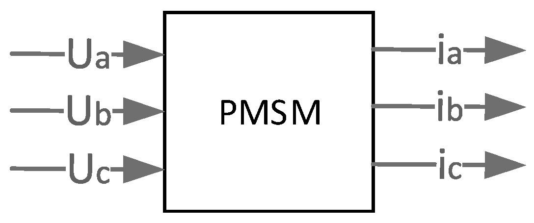
4.2. Modeling of PMSMs

The PMSM model is shown in Figure 10, where U a , U b , and U c denote the three-phase input phase voltages of the motor, and i a , i b , and i c denote the three-phase output stator currents of the motor. The PMSM modeling process finds the relationship between the output stator current and the input phase voltage. The derivation of this relation is described below.
After the coordinate transformation, U a , U b , and U c can be converted to the stator voltage U α of α -axes and the stator voltage U β of β -axes in the static coordinate system, as shown in Equation (8):
U α U β = 2 3 1 3 0 3 3 1 3 3 3 U a U b U c
U α and U β are converted to the stator voltage U d of the d-axis and the stator voltage U q of the q-axis in the rotating coordinate system, as shown in Equation (9):
U d U q = sin θ cos θ cos θ sin θ U α U β
By synchronously rotating Equation (9) in the coordinate system, Equations (10) and (11) are obtained:
U d U q = R i d i q + d d t φ d φ q + w e φ q φ d
φ d φ q = L d 0 0 L q i d i q + φ f 0
Here, R denotes the motor’s resistance, i d denotes the d-axis’s stator current, i q denotes the q-axis’s stator current, L d denotes the d-axis’s inductance, L q denotes the q-axis’s inductance, φ d denotes the d-axis’s stator flux, φ q denotes the q-axis’s stator flux, and φ f denotes the permanent magnet flux. The final current formula is as follows:
i d i q = 1 L d L q i d L q R + L q U d + φ q L q w e i q L d R + L d U q φ d L d w e
The i d and i q of the rotating coordinate system are converted to i α and i β :
i α i β = sin θ cos θ cos θ sin θ i d i q
After the coordinate transformation of i α and i β in the stationary coordinate system, three-phase stator currents i a , i b , and i c are obtained.
i a i b i c = 1 0 1 1 2 3 2 1 i α i β i 0
In practice, the performance of PMSMs is greatly affected by the rotor’s magnetic field space harmonics, magnetic circuit saturation, cross-saturation, and cross-coupling effects. In order to simulate the running state and performance of PMSMs more accurately, a general d q nonlinear model of PMSMs should be derived.
The steps of establishing the PMSM’s nonlinear model are as follows:
  • Step 1: The finite element method is used to obtain the relation curve of L d , L q , and φ f , changing with i d and i q , respectively. It should be noted that the finite element calculation method is the work of other members of the team, and the specific process is not described in this paper.
  • Step 2: Using the relationship curve obtained in step 1, the three parameters L d , L q , and φ f are obtained by looking up the table according to the current values i d and i q .
  • Step 3: The d q nonlinear model of the PMSM is obtained by substituting parameters L d , L q , and φ f into Equation (12).

4.3. Modeling of Flywheel

The mechanical equation of the flywheel is shown in Equation (15). Here, ω m denotes the rotor mechanical angular velocity of the PMSM, and B denotes the friction coefficient. T e denotes the electromagnetic torque of the PMSM, and T L denotes the drive torque of the PMSM.
T e T L = J d ω m d t + B ω m d θ m d t = ω m
The calculation formula for T e and T L is shown in Equation (16). Here, ψ f is the permanent magnet flux. i q is the d-axis current of the stator. P m is the number of poles of the PMSM.
T L = J d ω m d t T e = P m ψ f i q
In the case of ignoring mechanical loss, the output active power P f of the flywheel is equal to the electromagnetic power P e , as shown in Equation (17). It can be observed that the output active power of the flywheel is directly related to i q .
P f = P e = T e ω m = P m ψ f i q ω m

5. Modeling of Power Grids and Wind Farms

  • Modeling of power grids
According to the HIL testing system’s structure, as shown in Figure 2, a power grid test model was built. As shown in Figure 11, the power grid test model is equivalent to three AC voltage sources in parallel, and the output voltage is 35 kV before transformer processing. Here, U s A , U s B , and U s C denote three-phase AC voltage sources, R s denotes the equivalent resistance, and L s denotes the equivalent inductance. i s A , i s B , and i s C denote the phase current.
  • Modeling of wind farms
As shown in Figure 12, the wind farm test model is equivalent to three controllable current sources in parallel. Here, i A _ W F , i B _ W F , and i C _ W F denote three-phase controllable current sources, and the output value of the current source is shown in Equation (18). V n o m denotes the rated voltage of the power grid, and its value is 35 kV. θ g denotes the voltage angle of the power grid. As shown in Figure 2, θ g can be obtained from the three-phase voltage of the power grid through a PLL (phase-locked loop) operation. P W F is the current source power, simulating the active power output of the wind farm under wind speed fluctuations.
i A _ W F   = P W F V n o m sin ( θ g ) i B _ W F   = P W F V n o m sin ( θ g 2 * π / 3 ) i c _ W F   = i A _ W F i B _ W F

6. HIL Testing System Experiment

As mentioned above, the research focus of this article is the establishment of an FESS simulation model, rather than the development of FESS control algorithms. Therefore, in order to verify the correctness of the established FESS simulation models, the same FESS control algorithm developed by other members of the team was used in all following experiments. The aim of the experiments conducted with respect to the HIL testing system is to verify the following three points:
  • The correctness of the motor-side models in FESSs;
  • The correctness of the network-side models in FESSs;
  • The effectiveness of the power control function of FESSs for wind farms.
The experimental conditions are as follows. The dSPACE real-time simulator consists of four CPU boards and six FPGA boards. Among them, the CPU boards comprise DS1007, and the calculation steps are 1 × 10⁻⁸ s. The FPGA boards are DC5203, and they contain 12 high-resolution 14-bit analog-to-digital and digital-to-analog converters and 32 high-speed digital IO channels. The processing chip of DC5203 is Xilinx’s Kintex7 xc7k325t-1 fbg900, with a data rate of 6.6 Gb/s, which can be used for high-speed model calculations and simulations. Each board is connected through a peripheral high-speed bus, and the data transmission speed is 1.25 Gb/s. Because the electrical interface of the real-time simulator cannot be directly connected to the physical controller due to the voltage specification, a dSPACE signal conditioning unit is used to realize the signal’s conversion. The signal conditioning unit is equipped with various plug-ins to complete the conversion between different signals. Three 4 MW/125 kWh flywheel units are adopted in the system, and the selected parameters are shown in Table 1.

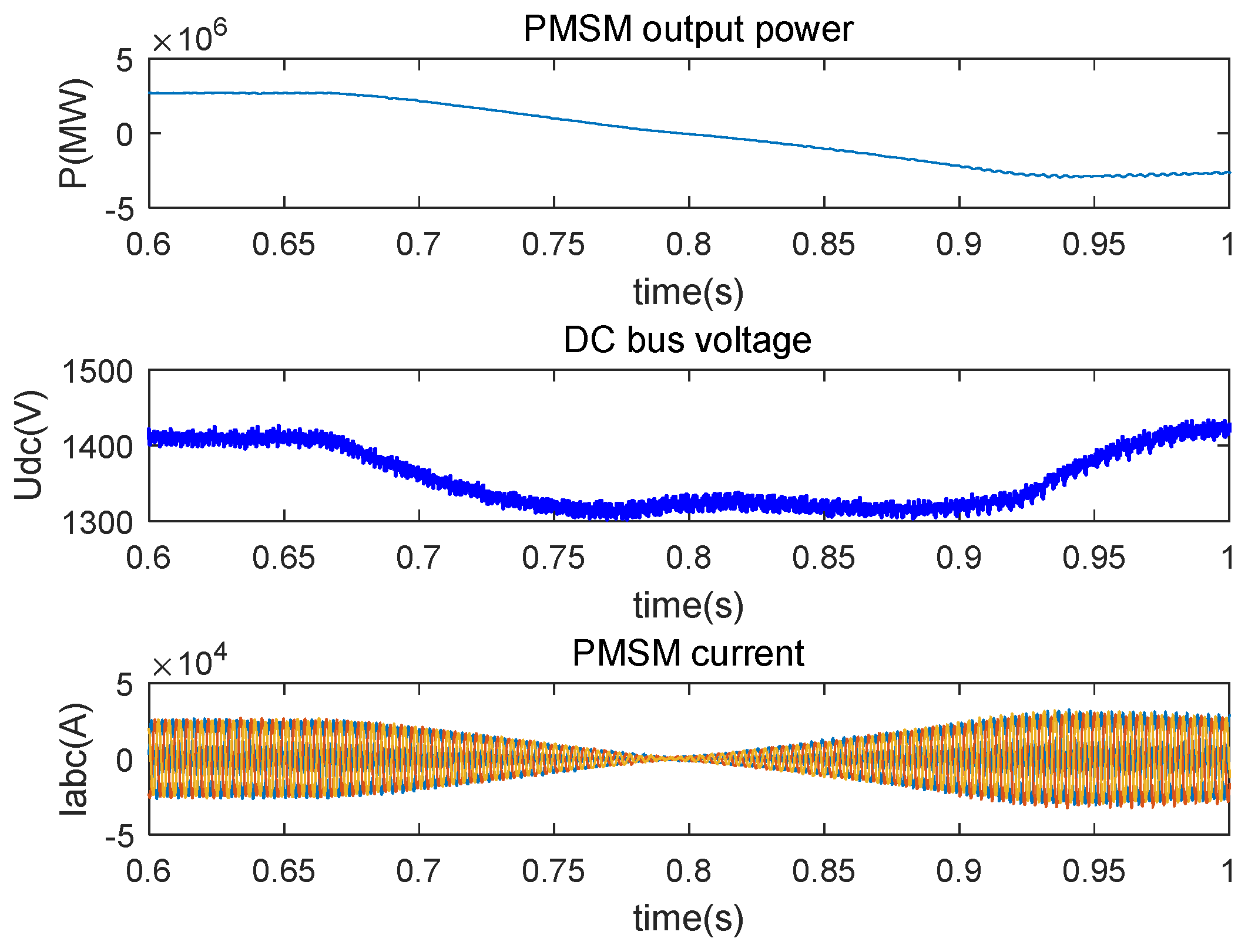
6.1. Verification of Motor-Side Models

In order to verify the correctness of motor-side models, the FESS process from the energy-charging state to the energy retention state and then to the energy-discharging state was simulated. As shown in Figure 13, at 0.6 s, the FESS is in the energy charging state, and the PMSM output power is rated at 4 MW. At 0.8 s, the FESS is in the energy retention state, and the PMSM output power is 0 kW. At 1 s, the FESS is in the energy-discharging state, and the PMSM output power is −4 MW. The DC bus voltage waveform is shown in Figure 13. When the FESS is in the energy charging state, energy flows out of the power grid. When the FESS is in the energy-discharging state, energy flows to the power grid. When the FESS switches from the charging to the discharging state, the resulting change in the direction of energy causes the DC bus voltage to decrease. At 0.8–1 s, when the FESS turns into the discharging state, the system outputs energy to the power grid, and the DC bus voltage also increases. The current waveform of the PMSM is shown in Figure 13. It is obvious that when the FESS completes the state switch at 0.8 s, the motor current is also reversed. As mentioned above, it can be observed that the motor-side models can realize the three-state switching of the FESS, which is consistent with the expected function. This shows the correctness of the motor-side models.

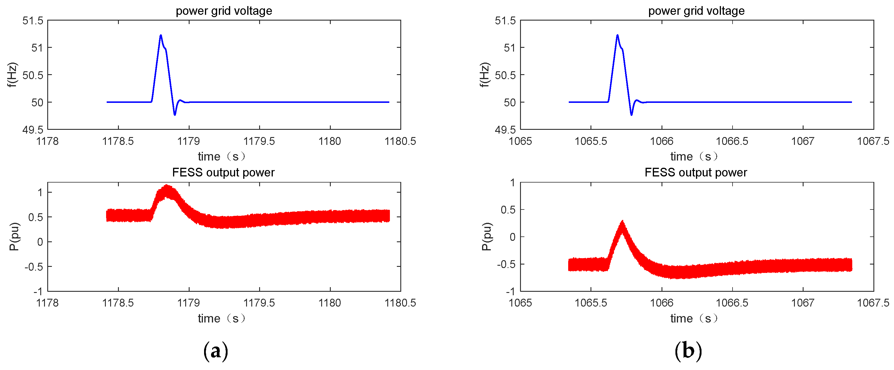
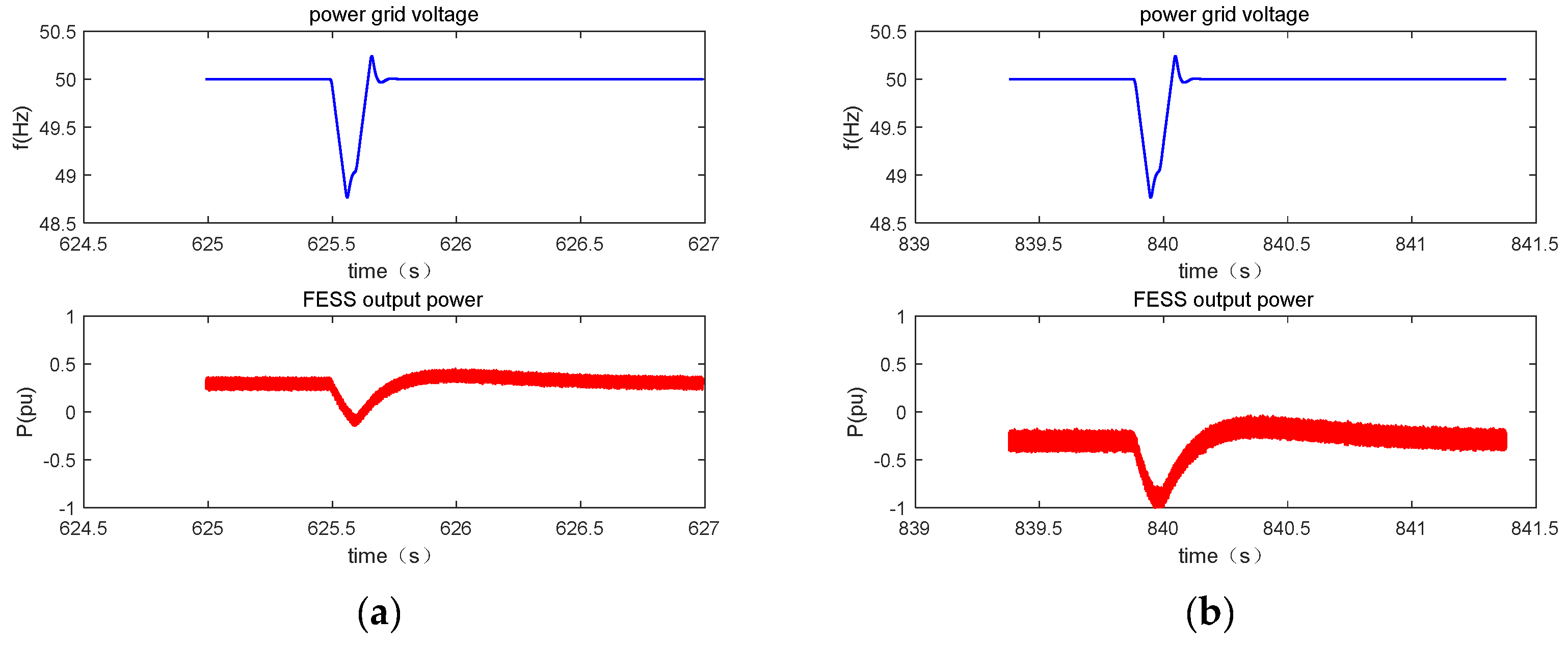
6.2. Verification of Network-Side Models

The output power of the FESS is adjusted when the voltage frequency of the power grid changes. The specific adjustment strategy is shown in Figure 14. In order to verify the power regulation effect of FESSs on wind farms, the step disturbance can be set in the voltage of the power grid to observe the power changes in the FESS.
  • Positive disturbance
When the voltage disturbance signal is positive, if the FESS is in the charging state, the charging power should be increased according to the power adjustment strategy from experience, as shown in Figure 14. It can be observed in Figure 15a that when the frequency of the power grid voltage is disturbed and increased to 51 Hz, the charging output power of the FESS increases. This is in line with the expected effect. When the voltage disturbance signal is positive, if the FESS is in the discharging state, the discharge power should be reduced according to the power adjustment strategy from experience, as shown in Figure 14. It can be observed in Figure 15b that when the frequency of the power grid voltage is disturbed and increased to 51 Hz, the discharge output power of the FESS decreases. This is in line with the expected effect.
  • Negative disturbance
When the voltage disturbance signal is negative, if the FESS is in the charging state, the charging power should be reduced according to the power adjustment strategy as shown in Figure 14. It can be observed in Figure 16a that when the frequency of the power grid voltage is disturbed and decreases to 49 Hz, the charging output power of the FESS decreases. This is in line with the expected effect. When the voltage disturbance signal is positive, if the FESS is in the discharge state, the discharge power should be increased according to the power adjustment strategy from experience, as shown in Figure 14. As shown in Figure 16b, the discharge output power of the FESS increases when the frequency of the power grid voltage is disturbed and decreases to 49 Hz. This is in line with the expected effect.

6.3. Verification of Power Control in Wind Farms

An array of three 4 MW/125 kW·h FESS units is used to match a 120 MW wind farm. As mentioned above, the output power of the wind power system can be simulated via the adjustment of the P W F of the wind farm model in Equation (18). A smoothing simulation was carried out for the wind power output within 180 min, and the results are shown in Figure 17. After the smoothing operation, the fast fluctuations in wind power output were significantly reduced.

7. Conclusions

In this paper, an HIL testing system was built for wind farm power control systems with FESSs. Firstly, the principle and structure of the system were analyzed. Then, the FESS, wind farm test, and power grid test models were analyzed and built. The modeling of the FESS main circuit and PMSM was the focus of this paper. Finally, the models were imported into the HIL testing system in order to carry out HIL experiments. The following conclusions can be drawn from the HIL experiments:
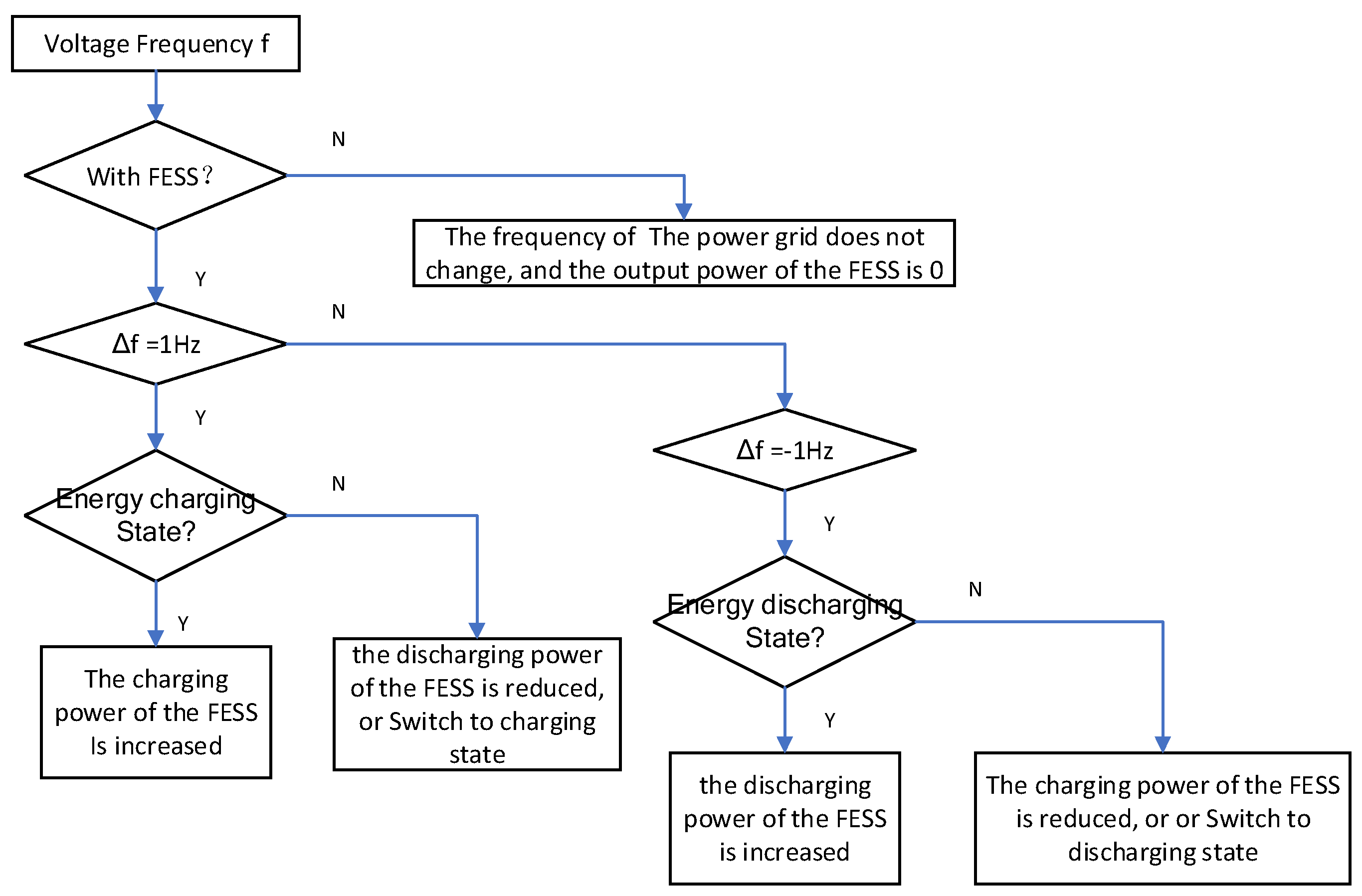
  • The constructed FESS model can realize the switching of three states—energy charging, energy discharging, and energy retention—which is in agreement with the expected theory.
  • The output power of FESS can be adjusted according to the voltage fluctuations of the power grid, and finally, the rapid fluctuations of the output power of the wind farm can be smoothed via the FESS, which is conducive to improving the wind farm’s grid connection rate.
  • The smoothing effect on wind farm output power indicates the reliability of the FESS algorithm in this experiment.
  • In general, the HIL testing system built in this article can provide a more convenient environment for the optimization of the team’s FESS control algorithm.
There is one limitation to the present study, which is the lack of a comparison of the current model with field data. Nevertheless, this study still shows the effectiveness of FESSs with respect to wind farm power control. In the future, we will further optimize the models based on field data in order to provide a more realistic simulation environment for the optimization of FESS control algorithms.

Author Contributions

Conceptualization, L.Y. and Q.Z.; methodology, L.Y.; software, L.Y.; validation, Q.Z.; formal analysis, L.Y.; investigation, Q.Z.; resources, L.Y.; data curation, L.Y.; writing—original draft preparation, L.Y.; writing—review and editing, Q.Z.; visualization, Q.Z.; supervision, Q.Z.; project administration, L.Y.; funding acquisition, L.Y. All authors have read and agreed to the published version of the manuscript.

Funding

This research was funded by the Hunan Provincial Natural Science Foundation of China, grant number 2022JJ60073.

Data Availability Statement

Further inquiries can be directed to the corresponding authors.

Conflicts of Interest

The authors declare no conflicts of interest. The funders had no role in the design of the study; in the collection, analyses, or interpretation of data; in the writing of the manuscript; or in the decision to publish the results.

Nomenclature

FESSFlywheel energy storage system
HILHardware-in-the-loop
PMSMPermanent magnet synchronous motor
ACAlternating current
IGBTInsulate gate bipolar transistor
ANPCActive neutral point clamped
PLLPhase-locked loop
ω Electrical angular velocity of the PMSM
θ Angular position of the PMSM
θ g Voltage angle of the power grid
i s a , i s b , i s c Three-phase stator current of the PMSM
U a , U b , U c Three-phase phase voltage of the PMSM
i u , i v , i w Three-phase current of the network-side inverter
U u , U v , U w Three-phase voltage of the network-side inverter
U g a , U g b , U g c Three-phase voltage of the power grid
S a , S b , S c PWM control signals of the motor-side inverter
S u , S v , S w PWM control signals of the network-side inverter
i g d The d-axis current of the network-side inverter
i g q The q-axis current of the network-side inverter
U d * The given d-axis voltage of the network-side inverter
U q * The given q-axis voltage of the network-side inverter
i d The d-axis stator current of the PMSM
i q The q-axis stator current of the PMSM
i d * The given d-axis stator current of the PMSM
i q * The given q-axis stator current of the PMSM
P f * The given active power of the PMSM
P d The given active power of the wind farm
Q f * The given reactive power of the PMSM
T f * The given torque of the PMSM
U d c The voltage of the DC bus

References

  1. The Law of the People’s Republic of China on Statistics Bulletin of the National Economy and Social Development in 2023. Available online: https://www.gov.cn/lianbo/bumen/202402/content_6934935.htm (accessed on 19 August 2024).
  2. Olabi, A.G.; Wilberforce, T.; Abdelkareem, M.A.; Ramadan, M. Critical Review of Flywheel Energy Storage System. Energies 2021, 14, 2159. [Google Scholar] [CrossRef]
  3. Xu, K.; Guo, Y.; Lei, G.; Zhu, J. A Review of Flywheel Energy Storage System Technologies. Energies 2023, 16, 6462. [Google Scholar] [CrossRef]
  4. Ji, W.; Hong, F.; Zhao, Y.; Liang, L.; Du, H.; Hao, J.; Fang, F.; Liu, J. Applications of flywheel energy storage system on load frequency regulation combined with various power generations: A review. Renew. Energy 2024, 223, 119975. [Google Scholar] [CrossRef]
  5. Li, Y.; Liu, S.C.; Yong, C.X. Modeling and Application of a Rectifier Transformer with Primary Winding in Series in A Metallurgical Rolling Mill System. Mechatron. Syst. Control 2023, 51, 182–192. [Google Scholar] [CrossRef]
  6. Zhang, J.W.; Wang, Y.H.; Liu, G.C.; Tian, G.Z. A review of control strategies for flywheel energy storage system and a case study with matrix converter. Energy Rep. 2022, 8, 3948–3963. [Google Scholar] [CrossRef]
  7. Floris, A.; Porru, M.; Damiano, A.; Serpi, A. Energy Management and Control System Design of an Integrated Flywheel Energy Storage System for Residential Users. Appl. Sci. 2021, 11, 4615. [Google Scholar] [CrossRef]
  8. Wang, B.; Yu, X.; Yang, X.; Zhang, D. Control strategy for high speed flywheel energy storage system based on voltage threshold of DC1500 V transit transportation traction grid. Energy Rep. 2022, 8, 640–647. [Google Scholar] [CrossRef]
  9. Lei, M.; Meng, K.; Feng, H.; Bai, J.; Jiang, H.; Zhang, Z. Flywheel energy storage controlled by model predictive control to achieve smooth short-term high-frequency wind power. J. Energy Storage 2023, 63, 106949. [Google Scholar] [CrossRef]
  10. Wang, K.; Tian, L.; Li, N.; Yin, X.; Han, L.; Jiang, T. Adaptive comprehensive control strategy for primary frequency regulation of coal-fired units assisted by flywheel energy storage system. J. Phys. Conf. Ser. 2023, 1, 2592. [Google Scholar] [CrossRef]
  11. Zheng, X.; Wu, Z.; Jia, Y.; Zhang, J.; Yang, P.; Zhang, Z. Fault-Tolerant Control Strategy for Phase Loss of the Flywheel Energy Storage Motor. Electronics 2023, 12, 3076. [Google Scholar] [CrossRef]
  12. Song, G.; Wu, Z.; Zheng, X.; Zhang, J.; Yang, P.; Zhang, Z. Control Strategy of Flywheel Energy Storage System for Improved Model Reference Adaptive System Based on Tent-Sparrow Search Algorithm. Electronics 2024, 13, 2699. [Google Scholar] [CrossRef]
  13. Qin, R.; Chen, J.; Li, Z.; Teng, W.; Liu, Y. Simulation of Secondary Frequency Modulation Process of Wind Power with Auxiliary of Flywheel Energy Storage. Sustainability 2023, 15, 11832. [Google Scholar] [CrossRef]
  14. Song, H.H.; Tian, D. Study on Hardware-in-the-loop-simulation of Wind Power Based on dSPACE. In Proceedings of the 2010 Second International Conference on Computational Intelligence and Natural Computing (CINC), Wuhan, China, 13–14 September 2010. [Google Scholar]
  15. Jia, Y.; Wu, Z.; Zhang, J.; Yang, P.; Zhang, Z. Control Strategy of Flywheel Energy Storage System Based on Primary Frequency Modulation of Wind Power. Energies 2022, 15, 1850. [Google Scholar] [CrossRef]
  16. Young, L.; Zheng, X.; Gao, E. Numerical Modeling and Application of Horizontal-Axis Wind Turbine Arrays in Large Wind Farms. Wind 2023, 3, 459–484. [Google Scholar] [CrossRef]
  17. Simani, S.; Farsoni, S.; Turhan, C. Hardware-In-The-Loop Assessment of a Fault Tolerant Fuzzy Control Scheme for an Offshore Wind Farm Simulator. IFAC PapersOnLine 2022, 55, 390–395. [Google Scholar] [CrossRef]
  18. Kikusato, H.; Ustun, T.S.; Suzuki, M.; Sugahara, S.; Hashimoto, J.; Otani, K.; Ikeda, N.; Komuro, I.; Yokoi, H.; Takahashi, K. Flywheel energy storage system based microgrid controller design and PHIL testing. Energy Rep. 2022, 8, 470–475. [Google Scholar] [CrossRef]
  19. Karrari, S.; De Carne, G.; Noe, M. Adaptive droop control strategy for Flywheel Energy Storage Systems: A Power Hardware-in-the-Loop validation. Electr. Power Syst. Res. 2022, 212, 108300. [Google Scholar] [CrossRef]
  20. Martínez-Nolasco, J.; Sámano-Ortega, V.; Botello-Álvarez, J.; Padilla-Medina, J.; Martínez-Nolasco, C.; Bravo-Sánchez, M. Development of a Hardware-in-the-Loop Platform for the Validation of a Small-Scale Wind System Control Strategy. Energies 2023, 16, 7813. [Google Scholar] [CrossRef]
  21. Venturini, S.; Cavallaro, S.P.; Vigliani, A. Windage loss characterisation for flywheel energy storage system: Model and experimental validation. Energy 2024, 307, 132641. [Google Scholar] [CrossRef]
  22. Huang, M.; Wang, Z.; Guo, Z.; Zeng, Q.; Niu, Y. Wind Tunnel Hardware-in-the-loop Simulation Techniques for Flight Control System Evaluation. In Proceedings of the 2017 2nd International Conference on Control Automation and Artificial Intelligence (CAAI), Sanya, China, 25–26 June 2017. [Google Scholar]
  23. Mathivanan, V.; Ramabadran, R.; Nagappan, B.; Devarajan, Y. Assessment of photovoltaic powered flywheel energy storage system for power generation and conditioning. Sol. Energy 2023, 264, 112045. [Google Scholar] [CrossRef]
  24. Wu, X.; Meng, Y.; Hu, S.; Song, B. Hardware-In-the-Loop Simulation of Wind Turbine Based on 6 Degree-of-Freedom Load. In Proceedings of the 2017 International Electrical and Energy Conference (CIEEC), Beijing, China, 25–27 October 2017. [Google Scholar]
Figure 1. Structural diagram of wind farms with FESSs.
Electronics 13 03610 g001
Figure 2. The structure of HIL testing systems.
Electronics 13 03610 g002
Figure 3. Circuit of the network-side inverter.
Electronics 13 03610 g003
Figure 4. Circuit of A-phase bridge arm.
Electronics 13 03610 g004
Figure 5. Circuit of a single IGBT: (a) original circuit; (b) equivalent circuit.
Electronics 13 03610 g005
Figure 6. Equivalent circuit of A-phase bridge arm.
Electronics 13 03610 g006
Figure 7. Equivalent circuit of the inductive filter.
Electronics 13 03610 g007
Figure 8. Equivalent circuit of the capacitive filter.
Electronics 13 03610 g008
Figure 9. Equivalent circuit of the support capacitor.
Electronics 13 03610 g009
Figure 10. PMSM model.
Electronics 13 03610 g010
Figure 11. Topological structure of the power grid test model.
Electronics 13 03610 g011
Figure 12. Topological structure of wind farm test models.
Electronics 13 03610 g012
Figure 13. Motor-side waveform.
Electronics 13 03610 g013
Figure 14. Power adjustment strategy from experience.
Electronics 13 03610 g014
Figure 15. FESS output power when there is positive disturbance: (a) under the charging state; (b) under the discharge state.
Electronics 13 03610 g015
Figure 16. FESS output power when there is negative disturbance: (a) under the charging state and (b) under the discharge state.
Electronics 13 03610 g016
Figure 17. Comparison of wind farm output power.
Electronics 13 03610 g017
Table 1. Parameters of the HIL testing system.
NumberParameterValue
1Rated frequency of power grid50 Hz
2Rated voltage of power grid35 kV
3Rated power of PMSM4 MW
4Rated voltage of PMSM3AC 850 V
5Rated current of PMSM2900 A
6Rated frequency of PMSM300 Hz
7Rated speed of PMSM5400 rpm
8Rated voltage of FESS1140 V
9Electric storage capacity of FESS125 kWh
Disclaimer/Publisher’s Note: The statements, opinions and data contained in all publications are solely those of the individual author(s) and contributor(s) and not of MDPI and/or the editor(s). MDPI and/or the editor(s) disclaim responsibility for any injury to people or property resulting from any ideas, methods, instructions or products referred to in the content.

