N-DEPTH: Neural Depth Encoding for Compression-Resilient 3D Video Streaming ^†

Abstract

Recent advancements in 3D data capture have enabled the real-time acquisition of high-resolution 3D range data, even in mobile devices. However, this type of high bit-depth data remains difficult to efficiently transmit over a standard broadband connection. The most successful techniques for tackling this data problem thus far have been image-based depth encoding schemes that leverage modern image and video codecs. To our knowledge, no published work has directly optimized the end-to-end losses of a depth encoding scheme sandwiched around a lossy image compression codec. We present N-DEPTH, a compression-resilient neural depth encoding method that leverages deep learning to efficiently encode depth maps into 24-bit RGB representations that minimize end-to-end depth reconstruction errors when compressed with JPEG. N-DEPTH’s learned robustness to lossy compression expands to video codecs as well. Compared to an existing state-of-the-art encoding method, N-DEPTH achieves smaller file sizes and lower errors across a large range of compression qualities, in both image (JPEG) and video (H.264) formats. For example, reconstructions from N-DEPTH encodings stored with JPEG had dramatically lower error while still offering 29.8%-smaller file sizes. When H.264 video was used to target a 10 Mbps bit rate, N-DEPTH reconstructions had 85.1%-lower root mean square error (RMSE) and 15.3%-lower mean absolute error (MAE). Overall, our method offers an efficient and robust solution for emerging 3D streaming and 3D telepresence applications, enabling high-quality 3D depth data storage and transmission.

1. Introduction

With the 2024 release of the Apple Vision Pro and its Persona digital avatar system, 3D telepresence has become more widely desired and accessible than ever. Apple’s Persona system is technically very impressive, but it does not stream any live-captured 3D data. Despite a recent proliferation of 3D capture hardware and advances in methods that allow for the real-time capture of 3D range data at high resolutions and frame rates, the vast majority of mainstream use cases can only use this data locally. This is because, without compression, a 3D data stream could be on the order of gigabits per second, a data rate that cannot be reliably sustained on a typical wireless broadband connection.

In order to encourage the development and adoption of novel 3D streaming use cases, such as 3D telepresence, performance capture, and telerobotics, more efficient methods of compressing this 3D information are required. Optimally, this 3D information could be stored in a way that allows compression by modern 2D image or video codecs, which are already highly optimized to exploit spatiotemporal redundancies and are very often hardware-accelerated. Unfortunately, values within a conventional depth image generally have higher bit depths (e.g., 16-bit, 32-bit) than color image channels, so they cannot be accurately compressed with the most common lossy image formats. Depth value bits can be directly split across multiple image channels, but this results in rapid spatial oscillations and discontinuities that do not compress well. Instead, an efficient, compression-resilient depth encoding scheme is required to smoothly and intelligently spread the depth information across the red, green, and blue color channels of a regular 2D image so that modern image and video codecs can be leveraged.

This paper proposes N-DEPTH, the first learned depth-to-RGB encoding scheme that is directly optimized for a lossy image compression codec. The key to this encoding scheme is a fully differentiable pipeline that includes a pair of neural networks sandwiched around a differentiable approximation of JPEG. An illustration of this pipeline can be seen in Figure 1. When trained end-to-end, the proposed system is able to minimize depth reconstruction losses and outperform a state-of-the-art, handcrafted algorithm. Furthermore, the proposed method is directly applicable to modern video codecs (e.g., H.264), making this neural encoding suitable for 3D data streaming applications.

Contributions

• We introduce N-DEPTH, a novel neural depth encoding scheme optimized for lossy compression codecs to efficiently encode depth maps into 24-bit RGB representations.
• We utilize a fully differentiable pipeline, sandwiched around a differentiable approximation of JPEG, allowing end-to-end training and optimization.
• We demonstrate significant performance improvements over a state-of-the-art method in various depth reconstruction error metrics across a wide range of image and video qualities, while also achieving lower file sizes.
• We offer a solution for emerging 3D streaming and telepresence applications, enabling high-quality and efficient 3D depth data storage and transmission.

In the remainder of this paper, Section 2 introduces related research up to the development of the proposed method, Section 3 describes the principle of the method, Section 4 provides experimental results for the method, Section 5 offers a discussion of the method, and Section 6 concludes the work. A preliminary version of this research was published in the proceedings of the 3D Imaging and Applications conference at the Electronic Imaging Symposium 2024 [1].

2. Related Work

Devices capable of reconstructing high-precision and high-resolution 3D geometry at real-time speeds have widely proliferated over the past decade [2,3]. Given this, such RGB-D and 3D imaging devices are being adopted within numerous applications in industry, entertainment, manufacturing, security, forensic sciences, and more. While the added spatial dimension has brought improvement to many domains, they are typically limited to working with the data at the capture source. That is, due to the high volume of data that 3D devices can produce, it is a practical challenge to store these 3D data or to transmit these 3D data to a remote location in real time [4] (e.g., for remote archival, processing, or visualization). Such functionality could be particularly beneficial for many applications, such as security, telepresence, entertainment, communications, robotics, and more. Given this, researchers have sought a robust and efficient method with which to compress 3D data.

While there has been much research proposed in the context of generic 3D mesh compression [5], such methods might unnecessarily impose too much overhead when the data to be compressed are produced by a single-perspective 3D imaging device. These devices (e.g., stereo vision, structured light, time-of-flight) often represent their data within a single depth map [6]. This depth map (Z) can be used to recover complete 3D coordinates (i.e., values $X(i,j)$ and $Y(i,j)$ for each $Z(i,j)$) if the imaging system’s calibration parameters are known. This means that if the depth map (Z) can be efficiently compressed then the 3D geometry can be recovered.

Storing only the depth map simplifies the task of 3D data compression. Since depth maps are often represented with 16-bit or 32-bit precision, whereas a regular RGB image typically uses 24 bits per pixel (i.e., 8 bits per channel), there are two prevailing approaches to storing depth maps as images. Some image-based depth encoding schemes ameliorate the bit-depth problem by using high dynamic range (HDR) image and video codecs. For instance, in Project Starline [7], a seminal 3D telepresence system, the depth streams were stored directly within the 10-bit luminance channels of a series of H.265 video streams. This, however, limited this system to a maximum of only 10 bits of precision for each depth stream. An alternative approach is to spread the depth map’s high bit-depth information over each of the red, green, and blue channels’ 8 bits. There have been a variety of approaches proposed for encoding 3D geometry data into the RGB values of a 2D image [8,9,10]. Ultimately, these methods attempt to intelligently distribute the 3D geometry’s data across the 2D output image’s RGB channels, such that (1) the resulting RGB image can be efficiently stored with 2D compression techniques and (2) the 3D geometry can be robustly reconstructed (i.e., decoded) from the signals in the compressed RGB channels.

Multiwavelength depth (MWD) [11] is one of the few state-of-the-art methods for encoding depth data across the red, green, and blue color channels of a typical RGB image that is robust to both lossless (e.g., PNG) and lossy (e.g., JPEG) image compression. Our previous work [12] also explored MWD’s robustness against various levels of video compression (i.e., H.264), using it to enable a real-time, two-way holographic 3D video conferencing application over standard wireless internet connections at 3–30 Mbps. MWD works by storing two sinusoidal encodings of the depth information, along with a normalized version of the depth information, into the RGB channels of a color image. More specifically, the red channel is a sinusoidal encoding of the normalized depth map, the green channel is a complementary cosinusoidal encoding, and the blue channel simply stores the normalized depth map. The frequency of the sinusoidal encodings can be tuned to balance compressibility and accuracy [13] (by adjusting MWD’s $n_{stairs}$ parameter), while the normalized depth map guides the phase unwrapping process during decoding. 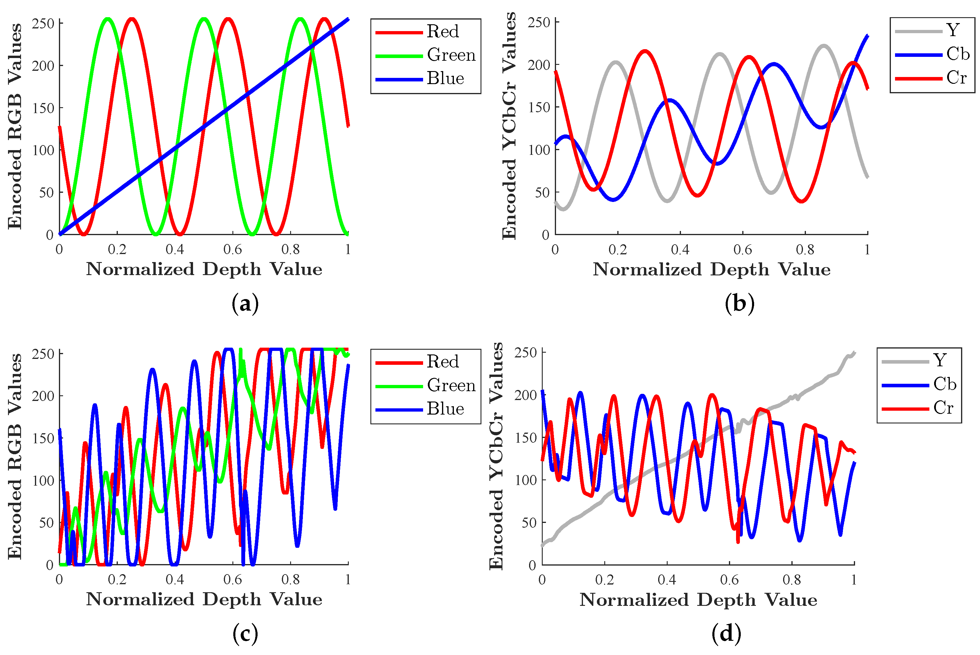Figure 2a illustrates how MWD encodes a normalized depth range across the red, green, and blue color channels when $n_{stairs}$ is set to 3, meaning that three periodic repetitions occur across the depth range (as can be seen in the encodings in the red and green channels).

While MWD proved to be quite efficient and robust against compression artifacts, subsequent works have attempted to decrease the effective file size of its compressed images by minimizing the number of encoding channels [14,15], reducing the depth range to be encoded [16], using a variable number of $n_{stairs}$ to offer a balance between targeted precision and improved compressibility [13,17], and decreasing the resolution of the output image [18]. In general, MWD’s ability to achieve small compressed file sizes while remaining robust against compression artifacts is due to its encodings being smoothly varying. That said, this handcrafted encoding scheme was never directly optimized for the image-compression codecs that it sought to exploit. While deep learning technologies have been used to train on a domain-specific dataset in the depth decoding pipeline of SCDeep [19] (another method derived from MWD), no published work in the area of depth-to-RGB encoding has leveraged deep learning throughout the entire encoding and decoding pipeline. This work proposes just that: an end-to-end image-based depth map compression method directly optimized for lossy image compression.

3. Methods

3.1. Overview

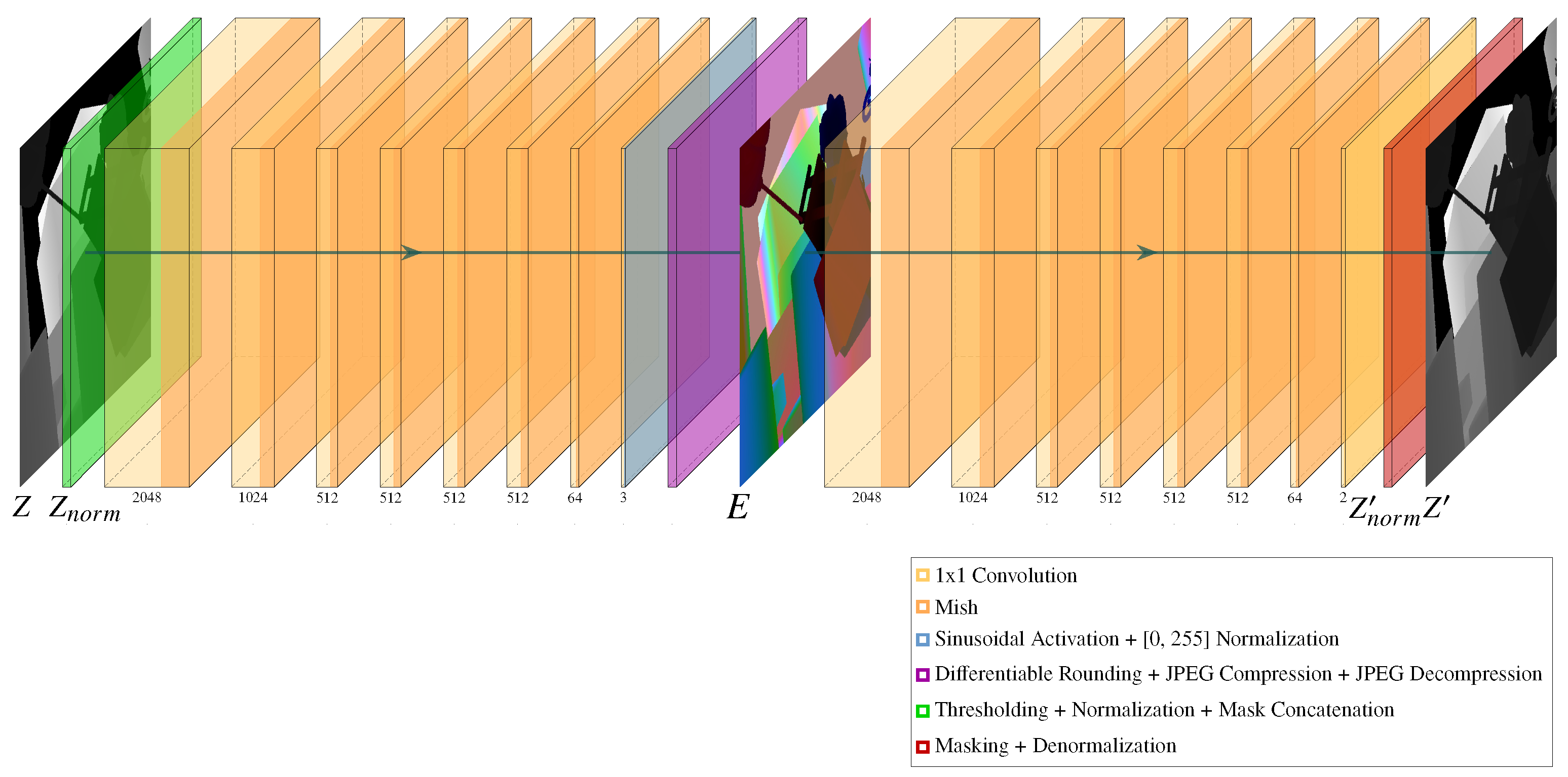
Figure 1 gives an overview of the full neural depth encoding, compression, and decoding pipeline. Fundamentally, this pipeline needs to take in a depth map, encode it into an RGB image, compress this image with a lossy codec such as JPEG, and then recover the depth map on the other end with as few end-to-end depth losses as possible. Unlike traditional, handcrafted algorithms that naively operate on the depth values to be stored, our encoding scheme leverages a pair of neural networks for the depth-to-RGB encoding and RGB-to-depth decoding, sandwiched around a differentiable approximation of JPEG compression. This system is, to our knowledge, the first depth-to-RGB encoding scheme that is directly optimized against a lossy image compression codec. Due to the exclusive use of 1 × 1 convolutions, the encoder and decoder neural networks can be succinctly understood as a pair of multilayer perceptrons (MLP) of similar structure. Together, they form N-DEPTH, a depth autoencoder where the bottleneck layer is an RGB image.

3.2. Encoding

Starting with a raw depth frame, the depth values are first thresholded within a desired depth range to form Z and then normalized to the range $[0,1]$ to form $Z_{norm}$. Additionally, values within the thresholding range are marked with a 1, while out-of-range values are marked with a 0 in a ground truth mask, which is concatenated to $Z_{norm}$ to form the input for the neural encoder network. The neural encoder employs a series of 1 × 1 convolutions that encode each depth and mask value pair into three floating-point numbers destined for the red, green, and blue color channels. Mish activations [20] are used in all layers except after the final encoder convolution, which uses a sinusoidal activation function. The sinusoidal activation primarily serves to restrict the outputs to the range $[-1,1]$. Additionally, experimental findings have indicated that using Mish and sinusoidal activation functions promotes faster and more optimal solution convergence compared to using only ReLU and sigmoid activations in the network. Finally, the outputs of the sinusoidal activation function are normalized to the $[0,255]$ range of an 8-bit unsigned integer, which ensures compatibility with the subsequent differentiable JPEG layer.

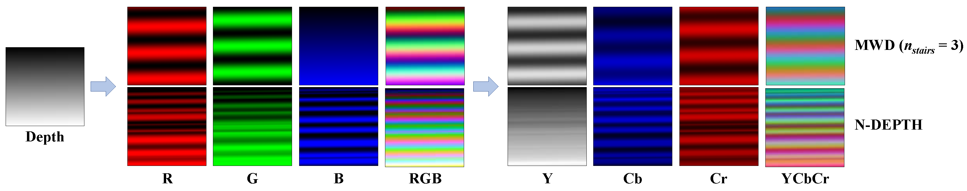
Figure 3 demonstrates how both N-DEPTH and MWD spread depth information across various color channels in both the RGB and YCbCr color spaces. The depth map being encoded here can be thought of as a tilted plane that samples the full $[0,1]$ normalized depth range, with a depth of 0 in the top-left corner and a depth of 1 in the bottom-right corner. MWD clearly exhibits smooth sinusoidal spatial oscillations in the red and green color channels, with the blue channel serving as a quantized version of the normalized depth map. In contrast, the N-DEPTH encoding appears to exhibit higher-frequency spatial oscillations than MWD in the RGB color space. However, when converted to the YCbCr color space, the luminance channel (Y) of the N-DEPTH encoding is largely smooth and approximates the original normalized depth map. In this YCbCr color space, N-DEPTH appears to encode the high-frequency information almost exclusively in the chrominance channels (Cb, Cr). Conversely, MWD exhibits sinusoidal oscillations in all channels of the YCbCr color space, without any strong specialization among the channels. These behaviors become even more starkly apparent in Figure 2. A parallel can clearly be drawn between the MWD RGB encoding scheme in Figure 2a and the N-DEPTH YCbCr encoding scheme in Figure 2d. N-DEPTH effectively stores an approximation of the normalized depth value in the luminance channel, very similarly to how MWD employs the blue channel to store a quantized version of the normalized depth value in the RGB color space. Furthermore, the chrominance channels of the N-DEPTH encoding plot strongly resemble the sinusoidal and cosinusoidal encoding pattern used by the red and green color channels in MWD.

More intuition about these encoding schemes can be gleaned by plotting their depth encoding functions in 3D. When plotted in an RGB color volume in Figure 4a, it becomes apparent that the equations defining MWD trace a helix that rotates about the blue color axis. Although the function is not as smooth, N-DEPTH also forms a distinctly helical shape that rotates about the luminance axis in Figure 4b. This learned behavior will be further discussed in Section 5.1.

3.3. Compression

In addition to being normalized to $[0,255]$, the outputs of the neural encoder need to be rounded to the nearest integer to simulate the quantization loss that occurs when attempting to store floating-point numbers in 8-bit color channels. Unfortunately, rounding is not a differentiable operation, so we need to use a differentiable quantizer proxy. We have elected to use the same “straight-through” quantizer proxy used in [21]. This quantizer proxy rounds inputs to the nearest integer during the forward pass but treats the operation as an identity function when calculating gradients during the backward pass of training. The lossless neural RGB encoding generated is next fed into a differentiable approximation of JPEG, DiffJPEG [22].

At this point, the bottleneck image of the autoencoder is an RGB encoding that has not yet been compressed. However, JPEG and most video codecs do not ordinarily store pixels in the RGB color space. Instead, a conversion to the YCbCr color space is more commonly used in lossy image and video-compression codecs. With JPEG, the “full-swing” version of YCbCr color space is ordinarily used, but video codecs usually use the “studio-swing” range for conversion to YCbCr. In this work, we will use the full-swing YCbCr range for both image and video compression for the sake of consistency, although the studio-swing conversions could also be employed at the cost of some numerical precision. In the YCbCr color space, the Y component represents luminance, which is the brightness of the grayscale information of the image. Humans are perceptually more sensitive to luminance information than chrominance, so the preservation of the luminance channel is often prioritized over the chrominance when performing lossy compression. We are focusing on JPEG image compression and H.264 video compression, both of which commonly employ 4:2:0 chroma subsampling of the YCbCr information to downsample the chrominance channels by a factor of 2 in both the horizontal and vertical directions. Since low-level control of chroma subsampling settings is often unavailable in video-streaming software solutions, all image and video compression methods in this paper employ 4:2:0 chroma subsampling for the widest-possible compatibility.

Note that we have modified the current publicly available version of DiffJPEG to use bilinear interpolation instead of nearest-neighbor interpolation for the chroma upsampling operation in order to more closely follow the JPEG specification. While training, there is no need to actually store a compressed JPEG file, so the lossless compression algorithms used in JPEG (i.e., run-length encoding and Huffman coding) are not explicitly simulated. After encoding and decoding are performed by DiffJPEG, the lossy RGB encoding E is generated, which has been normalized to a $[0,1]$ range in preparation for the neural decoding step.

3.4. Decoding

The neural decoder has a similar series of 1 × 1 convolutions as the encoder and takes the RGB encoding E as input. Mish activations are used after every 1 × 1 convolution in the decoder, with the exception of the final convolution, which directly outputs a two-channel image. These two channels correspond to a recovered mask and normalized depth map. During training, $Z_{norm}^{\prime }$ is recovered by applying the ground truth mask to the recovered depth channel. In contrast, for testing, the system applies a threshold to the recovered mask channel, which is then applied against the recovered depth channel to form $Z_{norm}^{\prime }$. It is the thresholded mask channel that is responsible for filtering the out-of-range background regions during testing. Lastly, the masked $Z_{norm}^{\prime }$ is denormalized back to the original depth range to recover $Z^{\prime }$.

3.5. Training

To enable the neural network to learn a compression-resilient encoding scheme across a variety of input depth maps, a diverse data set was chosen. FlyingThings3D [23] is a synthetic dataset of over 25,000 stereo image pairs of digital objects flying along randomized 3D trajectories. The included disparity maps were approximately inversely proportional to depth maps, so they were easily made into an acceptable substitute for training the neural depth autoencoder pipeline. The depth map analogs were randomly cropped and resized to 224 × 224 during training. Image histogram equalization was used to ensure relatively even sampling of the normalized depth range. A randomized threshold was applied to both the lower and upper bound of the depth range, after which the values were normalized. For training, the normalized depth range was expanded to $[-0.01,1.01]$ to improve the accuracy of depth reconstructions at the extrema of the $[0,1]$ testing inference range.

The JPEG quality levels were randomized and uniformly sampled from the range $[85,99.999]$. Periodic calibrations were performed during training in order to equalize the losses across the JPEG quality range, ensuring that training samples with low JPEG qualities did not dominate the losses and have an outsized impact on the solution convergence. An Adam optimizer with a cosine annealing learning rate scheduler with warm restarts [24] was used to minimize the L1 loss between $Z_{norm}$ and $Z_{norm}^{\prime }$ as well as the binary cross-entropy (BCE) loss between the ground truth mask and the recovered mask. In practice, the BCE loss was implemented as a single BCE with a logits loss layer that included an integrated sigmoid activation for improved numerical stability. Importantly, the original ground truth mask was not the exclusive source of data for training the outputs of the mask layer. Instead, a new form of ground truth mask was created by removing from the original ground truth mask those regions where the inferred depth had errors exceeding 3% of the normalized depth range. This combined mask enabled N-DEPTH to effectively filter out both background pixels and pixels whose RGB values it had low confidence in accurately decoding into depth. Using PyTorch (v2.3), the model was trained to convergence with an NVIDIA GeForce RTX 4090 with a batch size of 1.

The cosine annealing learning rate scheduler with warm restarts was configured with a period of 5000 iterations, after which the learning rate restarted to its full original learning rate ($1\times {10}^{-4}$). This is a relatively aggressive learning rate schedule that helps to find solutions closer to the global minimum in a difficult-to-navigate loss landscape. Due to the thorough sampling of the input parameter space and data-augmentation techniques, we did not encounter issues with overfitting. Since end-to-end numerical precision was very important to the accuracy of the depth map recoveries, we employed a progressive training approach with increasing precision levels. The network was initially trained using mixed precision, followed by PyTorch’s default precision mode (which allows the use of TensorFloat32 tensor cores on recent NVIDIA GPUs for certain operations, which reduces numerical precision) and, finally, using full 32-bit floating-point precision for every operation. Each precision level was utilized until the loss metric plateaued. This approach allowed for faster initial training while ensuring high numerical precision in the final stages. Training took approximately three days to complete.

4. Results

4.1. Middlebury 2014 Still Image Results

We first evaluated both MWD and N-DEPTH on a high-resolution still image dataset. The Middlebury 2014 dataset [25] is a widely recognized benchmark in the field of stereo vision. It consists of high-resolution stereo image pairs along with their corresponding disparity maps. In order to avoid largely redundant data, only the disparity maps aligned with the left camera’s perspective were used in our evaluations. For this study, we combined the training and the “additional” datasets (i.e., the scenes that included ground truth disparity maps) for a total of 23 disparity maps to test against. Not every point in the disparity maps had a valid ground truth measurement, so these regions were treated as being outside the normalized depth range. To facilitate our depth encoding algorithms, we converted the disparity maps into depth map analogs by taking the reciprocal of the disparity values and normalizing them to the range $[0,1]$. This simple conversion caused a slight non-linear distortion of the depth measurements, but it sufficed for the purposes of this paper, since the depth encoding algorithms operated pixelwise. The depth map analogs were first encoded into RGB images by both MWD ($n_{stairs}=3$) and N-DEPTH. Our experiments showed that setting $n_{stairs}=3$ consistently yielded the lowest depth reconstruction errors for MWD across the datasets used in this study. Therefore, we used this setting for all the MWD results presented in this manuscript. The lossless encodings were then compressed with JPEG using the Python Imaging Library (PIL) with JPEG qualities ranging from 1 to 99. The compressed images were subsequently decompressed and decoded back into normalized depth map analogs for analysis.

To quantitatively assess the performance of the depth encoding methods with this dataset, we employed two metrics: mean absolute percentage error (MAPE) and normalized root mean square error (NRMSE). Each of these metrics were relative to the normalized depth range and are reported as percentages. These metrics allowed us to fairly compare encoding performance across various scenes, even when the actual depth ranges differed significantly. In addition, we needed to define a couple of metrics that would help describe the performance of the depth background filtering. Both MWD and N-DEPTH have a particular encoding color that they use to label out-of-range depth entries, whether that is due to there being no ground truth depth available at that location or simply because it is outside of the depth range being considered. We defined “recall” as the percentage of ground truth depth measurements recovered without being filtered as out-of-range background. When an in-range depth value was filtered out, we would refer to this as a failed depth recovery. Ideally, high recall is a good thing, but it can result in the recovery of unreliable measurements that it is better to filter out. In contrast, we defined “precision” as the percentage of recovered depth measurements corresponding to actual ground truth measurements. A high score on this metric indicated that the depth decoding algorithm was not misclassifying out-of-range depth locations and attempting to calculate a recovered depth value where it was inappropriate.

Figure 5 compares the performance of N-DEPTH and MWD on a vintage computer scene with a JPEG quality of 90. The lossless RGB depth encodings for MWD and N-DEPTH can be seen in the first column. These encodings were compressed with JPEG quality 90 and decoded back into a normalized depth map. The absolute percentage error maps can be seen in the second column. Figure 5b shows regions of significant error in the depth map reconstruction by MWD. These regions corresponded to pixels near the edges of the objects and the surrounding undefined depth regions. These were the regions that were most susceptible to JPEG compression artifacts, due to the sharp boundaries. MWD uses a black color to encode out-of-range depth values; however, the black-level thresholding was largely ineffective in these sorts of regions, resulting in sharp discontinuities clearly being visible in the error map. Ideally, these inaccurate depth value recoveries would have been filtered out, even if they had corresponded to a defined ground truth depth value, but Figure 5c shows that MWD only failed to recover two pixels. This resulted in an MAPE of 0.563% and an NRMSE of 3.744%, largely caused by the large, spiky errors mentioned above. The largest of these spikes was as large as 98.9% of the normalized depth range. In contrast, the N-DEPTH encoding shown in Figure 5d resulted in a largely clean error map in Figure 5e. The MAPE was only 0.0256% and the NRMSE was only 0.0523%. These excellent results are largely attributable to the filtering that can be seen in the failed depth recoveries map in Figure 5f. N-DEPTH was able to successfully filter out both the out-of-range background and almost all of the pixel locations where the error was anticipated to be high. The maximum error for N-DEPTH in a recovered depth entry was 7.07% of the normalized depth range.

In order to limit the influence of differing filtering methodologies, the MAPE and NRMSE metrics for the rest of this subsection only considered the shared intersection of the depth recovery regions of both MWD and N-DEPTH. This allowed for a fairer comparison of the interior reconstruction qualities, since they could then both benefit from the more robust filtering afforded by N-DEPTH. Figure 6 compares the performance of MWD and N-DEPTH across the entire 23-image Middlebury 2014 dataset and a range of JPEG qualities from 1 to 99. Even with the help of the N-DEPTH filtering algorithm, MWD still trailed N-DEPTH in terms of both MAPE and NRMSE across the entire range of considered image qualities after normalizing for the resultant bits per pixel (bpp) measure. This hints at the fact that N-DEPTH is more compressible and does not sacrifice its reconstruction quality for those file size savings. Overall, N-DEPTH JPEG file sizes were 29.8% smaller on average when compressed with an equivalent JPEG quality setting.

Table 1. Aggregate reconstruction results for 23 static depth maps from the Middlebury 2014 dataset [25]. All encoded depth maps were compressed using JPEG 90. To limit the influence of the differing built-in filtering capabilities of the two methods, the NRMSE and MAPE metrics were calculated considering only the shared intersection of the depth values recovered by the two methods.

Depth Encoding Method	Average JPEG File Size (kB)	NRMSE	MAPE	Recall	Precision
MWD ($n_{stairs}$ = 3)	776.7 (1.116 bpp)	1.0126%	0.0723%	99.31%	99.99%
N-DEPTH	538.4 (0.774 bpp)	0.0681%	0.0314%	97.09%	100.00%

dives deeper into the numbers for the entire Middlebury 2014 dataset when the depth encodings were compressed with JPEG quality 90. At this quality setting, N-DEPTH achieved an average compression ratio (CR) of 41.35:1 relative to the original floating-point depth maps. In contrast, MWD achieved a lower CR of 28.66:1 under the same conditions. Despite the JPEGs generated by N-DEPTH being on average 30.68% smaller at this quality setting and MWD receiving the benefit of N-DEPTH’s filtering, N-DEPTH easily outperformed MWD in terms of both MAPE and NRMSE. N-DEPTH had an NRMSE of only 0.0681%, while MWD had a much larger NRMSE of 1.0126%. N-DEPTH also had a lower MAPE of 0.0314% versus the 0.0723% MAPE of MWD. In terms of depth recall and precision, MWD had a much higher recall of 99.31%. However, this recall likely came at the expense of its MAPE and RMSE metrics, which were heavily affected by errors at the boundaries between objects and with the background. Both methods did well in terms of precision, meaning that neither algorithm misclassified many background image pixels.

4.2. 3D Video Results

One of N-DEPTH’s goals is to enable advanced 3D video applications that require the live transmission of 3D data. To accomplish this practically, one may seek to combine image-based depth map encoding with existing 2D video technologies (e.g., H.264, H.265), as they are quite mature, exploit both spatial and temporal relationships in the data, and are often hardware-accelerated.For this purpose, we also evaluated N-DEPTH’s performance on a 3D video (sequence of depth maps) as encoded into a standard video format.

In HoloKinect [12], a 19.4 s depth video of a seated, moving subject (representative of a telecommunications scenario) was recorded on a Microsoft Azure Kinect (Microsoft Corporation, Redmond, WA, USA) with a depth range of 800 mm (200 mm to 1000 mm) and a resolution of 1280 × 720. The sequence of 582 ground truth depth frames was encoded into two sets of encodings, one with MWD applied ($n_{stairs}=3$) and another with N-DEPTH applied. The encodings were then 2-pass-H.264-video-encoded, using FFmpeg (v7.0) [26] with a x264 encoder to a variety of target average bit rates. We employed 4:2:0 chroma subsampling and the full swing of the YCbCr color space. To evaluate performance, the lossy frames were then decompressed with FFmpeg and then decoded by their respective algorithms.

Figure 7 shows an example frame from this dataset as reconstructed from the encodings stored within a 10 Mbps video (0.362 bpp), a rate low enough to be streamed on a large range of wireless connections. Both depth encoding methods demonstrate reasonably accurate interior reconstruction qualities (as can be seen in the first row). However, there is a slightly noisy band that can be seen in the N-DEPTH rendering along the cheek. This corresponds to a normalized depth region where even a lossless recovery of the RGB value would be noisy, due to imperfections in the learned functions. It can be seen that MWD exhibits very large, visually distracting discontinuities along the edges, which would require further post-processing to remove. In comparison, N-DEPTH shows far fewer discontinuity artifacts, due to its robust learned filtering.

While the interior reconstruction accuracy of MWD may be viable, its naive encodings can result in errors in its phase unwrapping process; these decoding errors then propagate to very large depth spikes in its reconstructions. Figure 7 further suggests that N-DEPTH inherently learns how to appropriately generate its encodings and masks in a manner capable of avoiding edge artifacts that drive large rates of error. In Figure 7’s frame, for instance, MWD’s RMSE (root mean square error) was 56.316 mm with an MAE (mean absolute error) of 5.371 mm. For the same frame, N-DEPTH’s RMSE and MAE were 0.885 mm and 0.591 mm, respectively. Figure 8 further illustrates these findings. MWD’s error map in Figure 8b shows regions with larger errors around the edges of the data. These same regions are absent, or not as pronounced, in N-DEPTH’s error map shown in Figure 8e. Figure 8c shows that MWD did not struggle to recover depth values corresponding to the ground truth data. While theoretically advantageous, this means that MWD will naively attempt to recover all salvageable data, even if it is now very noisy, due to compression artifacts. N-DEPTH, on the other hand, fails to recover such depth values, as can be seen in Figure 8f. In essence, N-DEPTH effectively learns to filter out those pixels that would have caused large artifacts. One contributor to this is that N-DEPTH learns an optimized color to encode the background pixels, as seen in Figure 8d’s encoding. This choice potentially enables smoother color transitions between the data and its background.

While Figure 7 and Figure 8 show visual and analytical results for a single $1280\times 720$ frame,

Table 2. Aggregate depth reconstruction results for a 3D video dataset (582 frames, $1280\times 720$ resolution) captured with a Microsoft Azure Kinect. All encoded depth maps were compressed into an H.264 video at 10 Mbps (0.362 bpp). To limit the influence of the differing built-in filtering capabilities of the two methods, the RMSE and MAE metrics were calculated considering only the shared intersection of the depth values recovered by the two methods.

Depth Encoding Method	Average Bit Rate (Mbps)	Depth RMSE (mm)	Depth MAE (mm)	Depth Recall	Depth Precision
MWD ($n_{stairs}$ = 3)	10.00 (0.362 bpp)	6.029	0.711	100.00%	99.92%
N-DEPTH	10.09 (0.365 bpp)	0.899	0.602	99.26%	100.00%

provides aggregate results over the entire 582-frame depth video sequence. In general, the same outcomes hold. When both methods are video-encoded at the same effective bit rate of 10 Mbps (0.362 bpp), N-DEPTH significantly outperforms MWD in terms of reconstruction quality, both in terms of RMSE and MAE. These results generalize beyond 10 Mbps videos, as well. Figure 9 provides both aggregate MAE (Figure 9a) and RMSE (Figure 9b) plots for a wide range of target bit rates, from 0.25 Mbps to 15 Mbps (0.009 bpp to 0.543 bpp). In all settings, N-DEPTH provided lower error metrics, suggesting that the encoding strategy it learned through JPEG was able to generalize to lossy video encoding.

5. Discussion

5.1. Chroma Subsampling and Color Space Transformations

All of the results in this paper included 4:2:0 chroma subsampling of the YCbCr color space. As it turns out, this chroma subsampling was an incredible source of direction for N-DEPTH during training. The losses incurred by chroma subsampling drove N-DEPTH to form a helical encoding function that rotated about the luminance channel (as is seen in Figure 4b). Intuitively, this behavior can be understood as the losses in the chrominance channels driving N-DEPTH to store its “most significant bits” of the depth information in the luminance channel that was fully sampled. This is very similar to how MWD stores a normalized depth map in the blue channel. However, the helix defined by MWD’s encoding functions does not align with the luminance channel after the RGB-to-YCbCr color space transformation, so it does not exploit the full sampling of the luminance channel. The top row of Figure 10 shows the training progression of N-DEPTH when learning a depth-to-RGB encoding function. Immediately, when training started, the encoding functions began to exploit the luminance channel by aligning with it. Over time, the encoding functions became more complex, forming a more intricate helical structure. By the time the network had converged at a solution, this helix was very closely aligned with the luminance axis, which is shown as a grayscale cord in Figure 10e. A full video of the 3D plots generated over the course of this training session can be seen in Supplementary Video S1 (https://zenodo.org/records/11399505/files/N-DEPTH-RGB-Full.mp4), with a shorter time-lapse version available in Supplementary Video S2 (https://zenodo.org/records/11399505/files/N-DEPTH-RGB-15s.mp4). Note that this is not the same training session as presented earlier in this work, since those results were not logged every 500 training samples.

Although the neural network was able to train through RGB-to-YCbCr and YCbCr-to-RGB color space transformations when learning depth-to-RGB encoding functions, doing so did interfere with its ability to learn a smooth function. When we ran experiments that removed these color space transformations and directly trained in the full YCbCr color space, the helical encoding structure was much smoother. The results of one of these training sessions can be seen in the bottom row of Figure 10, which is plotted in a YCbCr color volume. The YCbCr color space is actually much larger than the RGB color space, so training directly in the YCbCr color space allowed a greater range of quantized YCbCr values to be leveraged. In addition, this color space allowed for much easier alignment with the luminance axis. In the RGB color space, the helix needed to traverse from the black corner of the RGB volume to the white corner, which geometrically interfered with the development of a helix with a consistent radius. In contrast, when learning in the YCbCr color space, N-DEPTH was able to form a much more ideal helical shape, as can be seen in Figure 10j. A full video of the 3D plots generated by this YCbCr-trained version of N-DEPTH are available in Supplementary Video S3 (https://zenodo.org/records/11399505/files/N-DEPTH-YCbCr-Full.mp4), with a shorter time-lapse version available in Supplementary Video S4 (https://zenodo.org/records/11399505/files/N-DEPTH-YCbCr-15s.mp4).

Importantly, if we removed chroma subsampling from the compression layer of N-DEPTH during training, it did not learn a helical depth encoding pattern. In fact, although the encoding functions could be very effective even without chroma subsampling, they did not form any kind of ordered helical structure in the color spaces.

5.2. Background Filtering

The most important feature of N-DEPTH compared to MWD is its much more robust filtering of background pixels. The training session used earlier in this paper landed on a reddish–brown color to denote background, out-of-range locations. This was similar to how MWD uses black pixel values to denote its background regions. However, in addition to classifying reddish–brown pixels as background, the decoder of N-DEPTH has also learned to quantify its confidence in the reliability of the depth measurement recoveries of other RGB values. Although this masking function is taught as a binary classification that includes an error threshold of 3% of the normalized depth range, in practice N-DEPTH learns a more continuous confidence map. This confidence map can be thresholded at $sigmoid\left(0\right)$, but we elected to use a $sigmoid\left(8\right)$ threshold in Section 4.1 and a $sigmoid\left(6\right)$ threshold in Section 4.2. This allowed for more aggressive filtering in those datasets, which was very effective at improving the average quality of the recovered depth entries and subsequent 3D renderings.

5.3. Performance

5.3.1. Neural Implementation (GPU)

The architectural choices for N-DEPTH were driven by the desire for a large, expressive network capable of learning complex encoding and decoding functions. The encoder and decoder model sizes were increased until diminishing returns were encountered in the end-to-end depth reconstruction accuracy, resulting in encoder and decoder MLPs with 3.45 million parameters each. Although these models were large, a thorough exploration of the limited pointwise input parameter space via carefully considered training data augmentation greatly reduced the risk of overfitting. Therefore, an aggressive learning rate scheduler was leveraged to refine the model up to full 32-bit floating-point levels of precision throughout the networks. This implementation came with a performance penalty over PyTorch’s default levels of numerical precision on recent NVIDIA GPUs, but it did allow for a measurable increase in end-to-end accuracy at higher image compression qualities. However, the neural architecture was intentionally designed to operate pointwise with a pair of MLPs with very low input and output dimensionality. This architecture opened the possibility for the learned N-DEPTH encoding and decoding algorithms to be distilled down to a set of lookup tables or function approximations. A side benefit of the three-channel RGB outputs of the depth encoder was that the depth encoding functions could easily be graphed in three dimensions for a better geometric understanding of the learned encoding algorithm.

While computationally intensive, the neural implementation of N-DEPTH is able to run on consumer hardware with high-definition depth map inputs. In this discussion subsection, all performance metrics were evaluated on a Windows 11 desktop PC with an Intel Core i9-12900K and an NVIDIA GeForce RTX 4090. The encoder and decoder of N-DEPTH each required 3.45 million multiply–accumulate operations (MACs) per pixel, with the computational cost scaling linearly with the total size of the input depth map. The neural implementations were optimized for inference using TorchScript’s tracing mechanism. The resulting serialized versions of the models were then used to conduct performance benchmarks, primarily leveraging the GPU. These runtime performance evaluations focused on randomized input tensors with 1280 × 720 spatial dimensions, similar to the resolution of the Microsoft Azure Kinect depth maps used in Section 4.2. The N-DEPTH encoder inputs had a channel depth of 2, with the depth channel entries being randomly and uniformly sampled from the range $[0,1]$ and the binary mask channel entries having equal probabilities of being 0 or 1. In contrast, the N-DEPTH decoder inputs had a channel depth of 3, corresponding to red, green, and blue color channels. These pixels had their subpixel values randomly and uniformly sampled from the integer range $[0,255]$, with a subsequent normalization to the floating-point range $[0,1]$. No image or video compression was explicitly performed for the benchmarks in this section. In terms of memory usage, the encoder and decoder networks each utilized 11.9 GB of VRAM on the GPU at these input resolutions. Averaged over 1000 random tensors of size $[2,720,1280]$, an N-DEPTH encoder network inference takes 236.4 ms per frame, allowing for a maximum possible frame rate of 4.231 frames per second (FPS) on this hardware, if we ignore the computation required for preprocessing data and compressing the final output. Averaged over 1000 random tensors of size $[3,720,1280]$, an N-DEPTH decoder inference takes 237.2 ms per frame, for a maximum possible decoding frame rate of 4.217 FPS, if the overhead from decompression and postprocessing are ignored. These inference times are clearly too slow to allow for real-time use with a live 1280 × 720 depth video stream.

5.3.2. Lookup Table Implementation (CPU)

To provide an alternative to the burdensome computational demands of the neural implementation of N-DEPTH, we explored an approach that uses lookup tables (LUT). The depth encoding LUT contains $2^{16}$ entries (matching the maximum bit depth of Microsoft Azure Kinect measurements), with each entry storing 3 bytes for RGB values. This LUT was used to look up the proper encoded RGB values for any depth value in the normalized depth range. Any input depth that was outside of the specified depth range defaulted to a specific reddish–brown color that was learned by N-DEPTH to denote depth locations that should be filtered out during decoding. The decoding LUT included ${256}^3$ entries (one entry for each possible quantized RGB combination), each containing two single-precision floating-point values, one for the recovered normalized depth and one for the recovered mask value (which could be adjustably thresholded). The encoder LUT required only 196.6 kB of storage, while the decoder LUT required 134.2 MB. Although the LUT implementation of N-DEPTH was run in Python, it was optimized for runtime performance with a Numba [27] just-in-time compilation of the heavily multithreaded encoding and decoding functions. These functions ran on the CPU, without the GPU being utilized. Identical to the benchmarking of the neural implementation of N-DEPTH, the performance of the LUT implementation was averaged over a set of 1000 random input tensors for both the encoder and decoder. The LUT implementation of the N-DEPTH encoder was able to process a frame in only 0.847 ms for a maximum achievable encoding frame rate of 1180.8 FPS. The LUT decoder was similarly fast, with a decoding time of only 1.583 ms for a maximum achievable decoding frame rate of 631.6 FPS. These results demonstrate the potential for the use of N-DEPTH within real-time applications.

5.4. Limitations

While N-DEPTH demonstrates promising results, it is important to acknowledge its limitations in the areas of computational efficiency, precision, and spatial awareness. Importantly, this work was intended as an exploratory study rather than an implementation paper, focusing on optimizing reconstruction quality rather than runtime performance. The neural implementation of N-DEPTH was designed to be large and expressive, in order to optimize the reconstruction results of offline evaluations. Consequently, the neural networks are computationally expensive to run, especially at higher depth map resolutions. For real-time depth map streaming applications, more efficient implementations of N-DEPTH are necessary. The LUT-based N-DEPTH implementation described in Section 5.3 illustrates one approach to performance optimization. Additionally, smaller MLPs or alternative, more efficient neural architectures could be employed for application areas where neural runtime performance is critical.

Despite the large capacity of the encoder and decoder MLPs, the expressivity and precision of N-DEPTH are constrained by several factors. The requirement for end-to-end differentiability in the training pipeline limits the network’s ability to learn certain types of encoding functions, potentially excluding some optimal solutions. Training N-DEPTH to learn a smooth encoding function proved challenging, particularly due to the need to learn through color space conversions. The shape and orientation of the RGB color volume when transformed into the YCbCr color space made it difficult to form an ideal helical encoding structure aligned with the luminance axis. In contrast, learning directly in the YCbCr color space produced smoother and more ideal helical encoding structures, as demonstrated in the bottom row of Figure 10.

Even with a perfectly smooth and optimal encoding pattern, an MLP has limitations in terms of how much floating-point precision can be maintained as the network becomes deeper. Every additional layer added to the model inevitably contributes to the compounding floating-point precision losses. For classification problems, this loss of precision is not as problematic, but N-DEPTH also aims to recover floating-point depth values as accurately as possible. This is the reason that N-DEPTH is refined with higher levels of numerical precision, using full 32-bit floating-point precision for every mathematical operation in the network, even though this comes with a performance penalty. Unfortunately, attempts to integrate neural techniques, such as dense blocks [28] or residual connections [29] (which can both potentially help to maintain the higher-precision context of earlier layers), largely failed to converge to acceptable levels of reconstruction accuracy.

Another limitation of N-DEPTH is its lack of spatial awareness, since the network operates pointwise. Incorporating spatial context could potentially improve the pipeline’s robustness against compression artifacts and enhance overall reconstruction quality. However, attempts to incorporate 3 × 3 convolutions to introduce spatial context largely failed to converge to competitive end-to-end reconstruction accuracies. Moreover, such spatial operations would interfere with the ability to distill the network into lookup tables or simple functions, which is crucial to runtime performance.

6. Conclusions

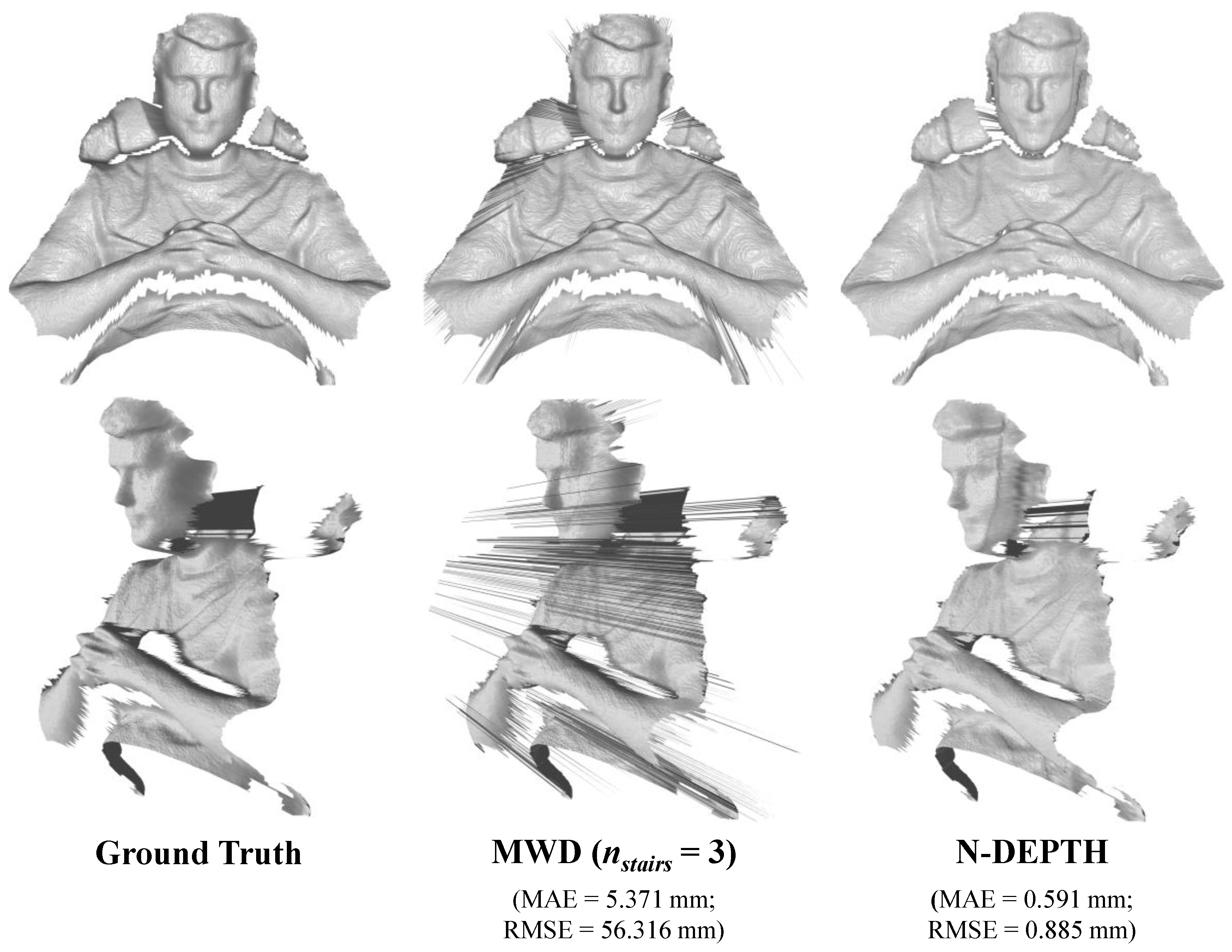
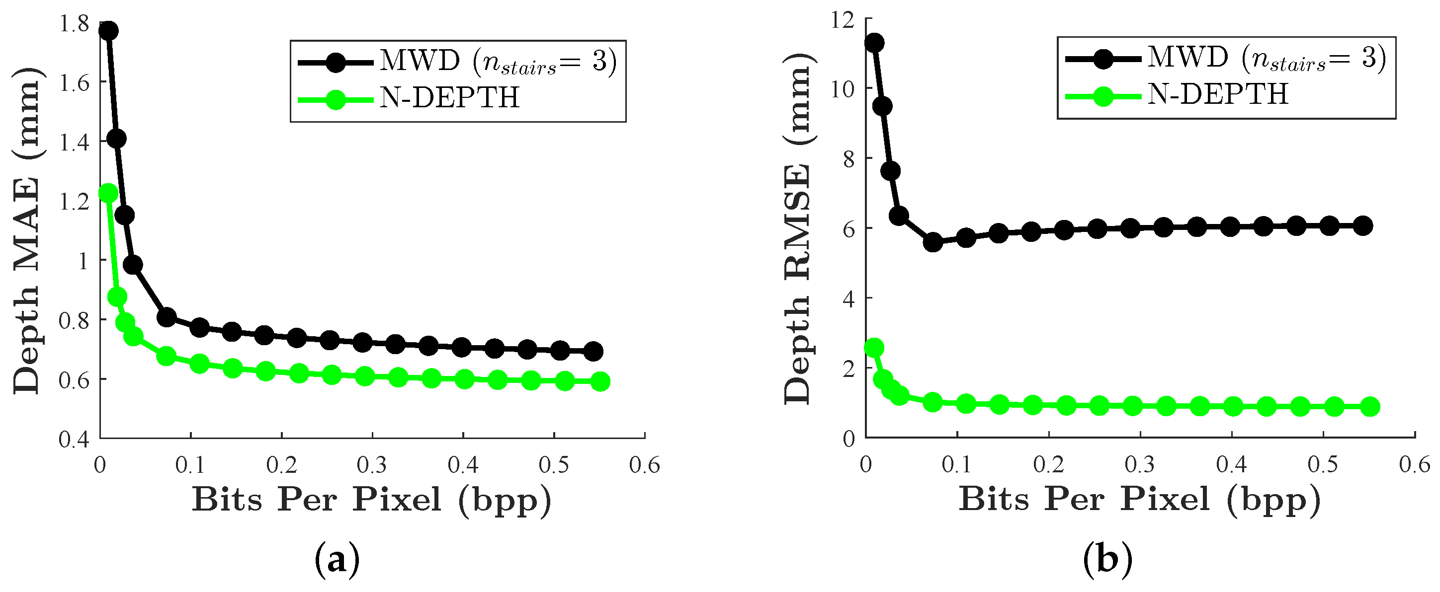
In summary, the proposed neural depth encoding method, N-DEPTH, demonstrates very promising results. To our knowledge, this is the first depth-to-RGB encoding scheme directly optimized for a lossy image compression codec. The learned depth encoding scheme consistently outperforms MWD, in terms of MAPE and NRMSE across a wide range of JPEG image qualities, and it achieves this with compressed image sizes that are, on average, more than 20% smaller. In addition, N-DEPTH similarly outperforms MWD, in terms of both MAE and RMSE, when sandwiched around H.264 video compression.

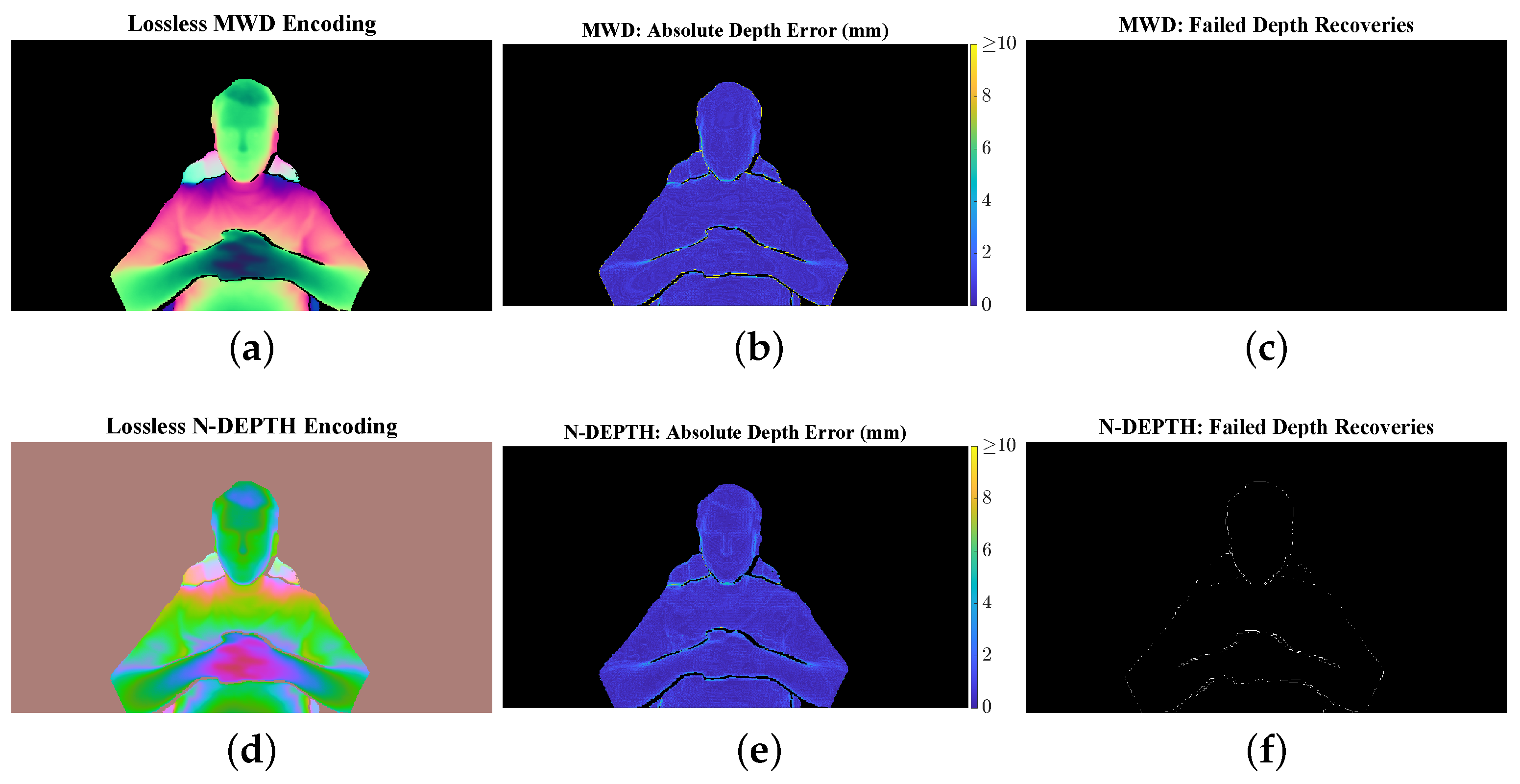
A key strength of N-DEPTH is its specialization in handling the types of errors that occur during lossy image and video compression, particularly artifacts derived from chroma subsampling and upsampling. This allows it to seamlessly integrate with off-the-shelf image compression and video streaming solutions. The method’s implicit filtering capabilities stand in stark contrast to those of MWD, since the filtering is so effective that further post-processing is essentially optional. However, a dedicated filtering neural network with spatial kernels could potentially further improve these results, albeit at the cost of increased computational complexity.

Future work could involve training N-DEPTH on a video compression analog, to better understand the temporal implications of compression artifacts. Matching the precision and quantization behavior of specific video codec implementations will also be important, particularly at higher quality levels. Additionally, the impact of using studio swing versus full swing in the YCbCr color space should be further investigated. While N-DEPTH shows excellent performance in applications involving color space transformations and chroma subsampling, MWD may still be better suited for scenarios without these operations.

The insights gained from N-DEPTH’s learned helical encoding strategy could drive the development of improved handcrafted depth encoding algorithms. It is worth noting that the neural network’s need for smoothness and differentiability may impose certain limitations on the functions it can learn. In addition, N-DEPTH is quite computationally complex to run, despite encoding smooth functions that could easily be approximated with a set of lookup tables or high-order polynomial approximations. Future research could explore the development of neural-inspired handcrafted algorithms that can more easily be implemented in real-time streaming applications. Overall, N-DEPTH offers a unique and effective solution for emerging 3D streaming and telepresence applications, enabling high-quality depth data storage and transmission in a manner that is resilient to lossy compression. The method’s learned encoding strategies provide valuable insights that can guide the development of even more advanced depth encoding techniques.

References

1. Siemonsma, S.; Bell, T. Neural Depth Encoding for Compression-Resilient 3D Compression. Electron. Imaging 2024, 36, 105-1–105-6. [Google Scholar] [CrossRef]
2. Zollhöfer, M.; Stotko, P.; Görlitz, A.; Theobalt, C.; Nießner, M.; Klein, R.; Kolb, A. State of the Art on 3D Reconstruction with RGB-D Cameras. Comput. Graph. Forum 2018, 37, 625–652. [Google Scholar] [CrossRef]
3. Marrugo, A.G.; Gao, F.; Zhang, S. State-of-the-art active optical techniques for three-dimensional surface metrology: A review. J. Opt. Soc. Am. A 2020, 37, B60–B77. [Google Scholar] [CrossRef]
4. Jang, E.S.; Preda, M.; Mammou, K.; Tourapis, A.M.; Kim, J.; Graziosi, D.B.; Rhyu, S.; Budagavi, M. Video-Based Point-Cloud-Compression Standard in MPEG: From Evidence Collection to Committee Draft [Standards in a Nutshell]. IEEE Signal Process. Mag. 2019, 36, 118–123. [Google Scholar] [CrossRef]
5. Maglo, A.; Lavoué, G.; Dupont, F.; Hudelot, C. 3D mesh compression: Survey, comparisons, and emerging trends. ACM Comput. Surv. (CSUR) 2015, 47, 1–41. [Google Scholar] [CrossRef]
6. Zhang, S. High-speed 3D shape measurement with structured light methods: A review. Opt. Lasers Eng. 2018, 106, 119–131. [Google Scholar] [CrossRef]
7. Lawrence, J.; Goldman, D.B.; Achar, S.; Blascovich, G.M.; Desloge, J.G.; Fortes, T.; Gomez, E.M.; Häberling, S.; Hoppe, H.; Huibers, A.; et al. Project Starline: A high-fidelity telepresence system; Project Starline: A high-fidelity telepresence system. ACM Trans. Graph 2021, 40, 16. [Google Scholar] [CrossRef]
8. Karpinsky, N.; Zhang, S. Composite phase-shifting algorithm for three-dimensional shape compression. Opt. Eng. 2010, 49, 063604. [Google Scholar] [CrossRef]
9. Zhang, S. Three-dimensional range data compression using computer graphics rendering pipeline. Appl. Opt. 2012, 51, 4058–4064. [Google Scholar] [CrossRef]
10. Ou, P.; Zhang, S. Natural method for three-dimensional range data compression. Appl. Opt. 2013, 52, 1857–1863. [Google Scholar] [CrossRef]
11. Bell, T.; Zhang, S. Multiwavelength depth encoding method for 3D range geometry compression. Appl. Opt. 2015, 54, 10684. [Google Scholar] [CrossRef]
12. Siemonsma, S.; Bell, T. HoloKinect: Holographic 3D Video Conferencing. Sensors 2022, 22, 8118. [Google Scholar] [CrossRef]
13. Finley, M.G.; Nishimura, J.Y.; Bell, T. Variable precision depth encoding for 3D range geometry compression. Appl. Opt. 2020, 59, 5290–5299. [Google Scholar] [CrossRef]
14. Finley, M.G.; Bell, T. Two-channel depth encoding for 3D range geometry compression. Appl. Opt. 2019, 58, 6882–6890. [Google Scholar] [CrossRef]
15. Finley, M.G.; Bell, T. Two-channel 3D range geometry compression with primitive depth modification. Opt. Lasers Eng. 2022, 150, 106832. [Google Scholar] [CrossRef]
16. Finley, M.G.; Bell, T. Depth range reduction for 3D range geometry compression. Opt. Lasers Eng. 2021, 138, 106457. [Google Scholar] [CrossRef]
17. Schwartz, B.S.; Finley, M.G.; Bell, T. Foveated 3D range geometry compression via loss-tolerant variable precision depth encoding. Appl. Opt. 2022, 61, 9911–9925. [Google Scholar] [CrossRef]
18. Schwartz, B.S.; Bell, T. Downsampled depth encoding for enhanced 3D range geometry compression. Appl. Opt. 2022, 61, 1559–1568. [Google Scholar] [CrossRef] [PubMed]
19. Finley, M.G.; Schwartz, B.S.; Nishimura, J.Y.; Kubicek, B.; Bell, T. SCDeep: Single-Channel Depth Encoding for 3D-Range Geometry Compression Utilizing Deep-Learning Techniques. Photonics 2022, 9, 449. [Google Scholar] [CrossRef]
20. Misra, D. Mish: A Self Regularized Non-Monotonic Activation Function. arXiv 2020, arXiv:1908.08681. [Google Scholar]
21. Guleryuz, O.G.; Chou, P.A.; Hoppe, H.; Tang, D.; Du, R.; Davidson, P.; Fanello, S. Sandwiched Image Compression: Wrapping Neural Networks Around A Standard Codec. In Proceedings of the 2021 IEEE International Conference on Image Processing (ICIP), Anchorage, AK, USA, 19–22 September 2021; pp. 3757–3761. [Google Scholar] [CrossRef]
22. Lomnitz, M.R. DiffJPEG. 2021. Available online: https://github.com/mlomnitz/DiffJPEG (accessed on 2 May 2024).
23. Mayer, N.; Ilg, E.; Hausser, P.; Fischer, P.; Cremers, D.; Dosovitskiy, A.; Brox, T. A large dataset to train convolutional networks for disparity, optical flow, and scene flow estimation. In Proceedings of the IEEE Conference on Computer Vision and Pattern Recognition, Las Vegas, NV, USA, 27–30 June 2016; pp. 4040–4048. [Google Scholar]
24. Loshchilov, I.; Hutter, F. SGDR: Stochastic Gradient Descent with Warm Restarts. arXiv 2016, arXiv:1608.03983. [Google Scholar]
25. Scharstein, D.; Hirschmüller, H.; Kitajima, Y.; Krathwohl, G.; Nešić, N.; Wang, X.; Westling, P. High-Resolution Stereo Datasets with Subpixel-Accurate Ground Truth. In Pattern Recognition; Jiang, X., Hornegger, J., Koch, R., Eds.; Springer International Publishing: Cham, Switzerland, 2014; pp. 31–42. [Google Scholar]
26. FFmpeg Developers. FFmpeg Multimedia Framework. Available online: https://ffmpeg.org/ (accessed on 11 May 2024).
27. Lam, S.K.; Pitrou, A.; Seibert, S. Numba: A LLVM-based Python JIT compiler. In Proceedings of the Second Workshop on the LLVM Compiler Infrastructure in HPC, LLVM’15, New York, NY, USA, 15 November 2015. [Google Scholar] [CrossRef]
28. Huang, G.; Liu, Z.; Van Der Maaten, L.; Weinberger, K.Q. Densely connected convolutional networks. In Proceedings of the IEEE Conference on Computer Vision and Pattern Recognition, Honolulu, HI, USA, 21–26 July 2017; pp. 4700–4708. [Google Scholar]
29. He, K.; Zhang, X.; Ren, S.; Sun, J. Deep Residual Learning for Image Recognition. In Proceedings of the Conference on Computer Vision and Pattern Recognition, Las Vegas, NV, USA, 27–30 June 2016; pp. 770–778. [Google Scholar]
Figure 1. The N-DEPTH encoding, compression, and decoding pipeline. The depth map Z is first thresholded to the desired depth range and normalized between 0 and 1 to form Z n o r m . A mask denoting the in-range and out-of-range regions is concatenated to Z n o r m to form the input to the neural depth encoder. The output of the neural encoder is fed into a differentiable JPEG approximation, which produces a lossy RGB encoding E. This is then fed into the neural decoder that recovers Z n o r m , which is denormalized to the original depth range to produce the final depth map reconstruction Z .
Electronics 13 02557 g001
Figure 2. Depth encodings along a normalized depth range as produced by MWD ( n s t a i r s = 3 ) and N-DEPTH. N-DEPTH appears to learn an encoding strategy similar to MWD, albeit within a different color space: (a,b) MWD encodings in the RGB and YCbCr color space, respectively. (c,d) N-DEPTH encodings in the RGB and YCbCr color space, respectively.
Electronics 13 02557 g002
Figure 3. Example lossless depth encodings of an ideal tilted plane. This figure demonstrates how MWD (Row 1) and the proposed N-DEPTH neural depth encoding method (Row 2) each spread the plane’s depth information across the red, green, and blue image channels. The left-hand side shows the encodings produced by each method in the typical RGB color space, and the right-hand side shows the encodings after transformation into the YCbCr color space (represented with grayscale, blue, and red pseudocolors, respectively).
Electronics 13 02557 g003
Figure 4. Encodings produced by MWD and N-DEPTH viewed within a color space volume: (a) MWD’s encodings of the normalized depth range [ 0 , 1 ] in the RGB color space. Each point on the curve represents an RGB color encoding of a specific depth value. (b) N-DEPTH’s encodings in the YCbCr color space. Each point represents a YCbCr color encoding of a specific depth value. N-DEPTH appears to learn a periodic encoding strategy similar to MWD (this learned behavior is further discussed in Section 5.1). The helical structures show how depth values are mapped to colors, with MWD’s helix rotating about the blue axis and N-DEPTH’s tighter helix primarily rotating about the Y (luminance) axis. Note that N-DEPTH’s helix in the YCbCr color space is narrower than MWD’s in the RGB space. This is due to the bounds of the RGB space, which restrict the range of encodings compared to the YCbCr space.
Electronics 13 02557 g004
Figure 5. Reconstruction performance for MWD and N-DEPTH on the vintage computer scene from the Middlebury 2014 dataset [25] with JPEG quality 90: (a) Lossless MWD encoding. (b) MWD absolute error map. (c) MWD failed depth recoveries. (d) Lossless N-DEPTH encoding. (e) N-DEPTH absolute error map. (f) N-DEPTH failed depth recoveries.
Electronics 13 02557 g005
Figure 6. Quantitative results over the entire 23-image Middlebury dataset when both MWD and N-DEPTH encodings were stored with JPEG qualities in the range [ 1 , 99 ] , with the resultant average bits per pixel (bpp) measures shown on the horizontal axes: (a) mean absolute percentage error (MAPE) plot. (b) normalized root mean square error (NRMSE) plot. In order to limit the influence of differing filtering methodologies, the MAPE and NRMSE metrics only considered the shared intersection of the depth recovery regions of both MWD and N-DEPTH.
Electronics 13 02557 g006
Figure 7. 3D renderings (front and side) from MWD and N-DEPTH. A 1280 × 720 Azure Kinect video frame was decoded from MWD and N-DEPTH encodings stored in an H.264 video at 10 Mbps (0.362 bpp).
Electronics 13 02557 g007
Figure 8. Reconstruction performance for MWD and N-DEPTH on a frame from the Azure Kinect dataset stored in 10 Mbps (0.362 bpp) H.264 video, as rendered in Figure 7: (a) Lossless MWD encoding. (b) MWD absolute error map. (c) MWD failed depth recoveries. (d) Lossless N-DEPTH encoding. (e) N-DEPTH absolute error map. (f) N-DEPTH failed depth recoveries.
Electronics 13 02557 g008
Figure 9. Quantitative results on a 582-frame 720P Microsoft Azure Kinect depth video: (a) mean absolute error (MAE) plot. (b) root mean square error (RMSE) plot. The encoded depth frames were 2-pass-H.264-video-compressed to a set of target average bit rates. A wide range of target average bit rates, from 0.25 Mbps to 15 Mbps, was tested, with the resultant bits per pixel (bpp) measures shown on the horizontal axes. The MAE and RMSE metrics were taken as aggregate measures over the entire video sequence. To limit the influence of differing filtering methodologies, the MAE and RMSE metrics only considered the shared intersection of the depth recovery regions of both MWD and N-DEPTH. MWD utilized an analytically optimized black level thresholding value of approximately 0.3326.
Electronics 13 02557 g009
Figure 10. Evolution of the depth encoding functions that N-DEPTH learned over the course of a pair of full training sessions: (ae) show the progress of N-DEPTH when trained in the RGB color space, with implicit color space transformations to and from YCbCr in the DiffJPEG compression layer; (fj) show the progress of N-DEPTH when trained directly in the YCbCr color space. Points on the curves are colored based on their positions in the RGB volume in (ae) and pseudocolored in the YCbCr volume in (fj).
Electronics 13 02557 g010