Fast Noise Level Estimation via the Similarity within and between Patches

Abstract

Patch level-based noise level estimation (NLE) is often inaccurate and inefficient because of the harsh criteria required to select a small number of homogeneous patches. In this paper, a fast image NLE method based on a global search for similar pixels is proposed to solve the above problem. Specifically, the mean square distance (MSD) is first expressed in the form of the standard deviation (std) and mean value of image patches. Afterward, the two values, std and mean, are calculated and stored in advance. Then, a 2D statistical histogram and summed area table are adopted to speed up the search for similar patches. Further, the most similar pixels are selected from similar patches to obtain an initial estimation. Finally, we correct the deviation of the initial estimation by re-injecting noise for secondary estimation. Experimental results show that the proposed method outperforms the state-of-the-art techniques in fast NLE and guided denoising.

1. Introduction

As a low-level machine vision operation, image noise level estimation (NLE) is an essential task that is widely used in many fields, such as denoising [1,2], compression [3], segmentation [4], image quality assessment [5], optical flow [6], image deblurring [7], object recognition [8], feature extraction [9], and super-resolution [10], and needs to be corrected according to the noise level. The performance of these algorithms strongly depends on the noise level, but the noise level is often unknown beforehand in practice. Therefore, developing an efficient, fast NLE technique is an important endeavor in image processing.

The commonly used strategies in NLE are the selection of homogeneous regions and noise statistical analysis. In terms of the method used for the selection of homogeneous regions [11,12,13,14,15,16,17,18,19,20,21], filtering-based methods [11,12,13,14,15] typically require a special filter to eliminate strong textures in the image, such as edges and other structural content; the majority of the remaining noise is pixel-independent, but due to changes in local texture, the noise level is easily overestimated, or if a small number of patches are selected, the noise level will be underestimated. In order to find sufficient homogeneous regions NLE, the authors in [16,17,18] use filters to search for pixel differences between patches, but their performance is largely affected by thresholds. Our previous work [19] searched for homogeneous regions by calculating the mode of patches to obtain stable estimation results, but this method is prone to overestimation in low-noise images with complex textures. As for the typical representation methods, the patch-based principal component analysis (PCA) method [20,21] has also achieved good results, but due to it only including small eigenvalues of some noise components, its estimated noise variance is usually smaller than the actual variance. Therefore, PCA-based estimators make it easy to underestimate variance, especially for low-frequency images with high noise levels.

In statistical methods, high-order moment invariance methods [22,23,24,25,26] usually require us to solve complex nonlinear optimization problems. In the global SVD methods [22], the noise level is estimated by counting the number of smaller singular values, but the noise subspace is difficult to find and requires a large amount of statistical data. Other statistical strategies [23] estimate noise levels by establishing the relationship between noise variance and statistics. The method in [24] utilizes the symmetry of the Gaussian distribution of noise to establish the relationship between patch redundancy eigenvalues and noise; when the mean and median of patch eigenvalues are equal, the eigenvalue of this position is the noise level. Therefore, NLE is converted into an estimate of the dimensionality of patch redundancy. However, this method performs poorly when dealing with images with complex textures. In summary, the accuracy of these methods depends on the number of homogeneous patches or the fine design of the model.

The key idea of the above methods is to separate the contribution of the image structure to the NLE results. Although carefully selected, the smallest unit is only patch-based, and still contains the image’s structure information. Therefore, Hou et al. [2] proposed a method to estimate the noise level based on the non-local self-similarity (NLE-NSS) of pixels and obtained better performance. However, this method is still a local strategy, i.e., it essentially searches for similar patches from the neighborhood, and its average output of all local estimates will overestimate the noise level.

Therefore, a novel method to accelerate the search for similar patches and pixels globally to estimate the noise level is proposed in this paper. Specifically, the mean square distance (MSD) is first expressed in the form of both the standard deviation (std) and mean of image patches. Then, the patch features, including the std and mean, are pre-calculated and stored to search for similar patches and pixels quickly. Finally, the NLE is extended from local to global. In particular, we further correct the deviation of the estimation results. The experimental results show that the proposed method is superior to the state-of-the-art methods in NLE and guided denoising. The contributions of this paper are as follows:

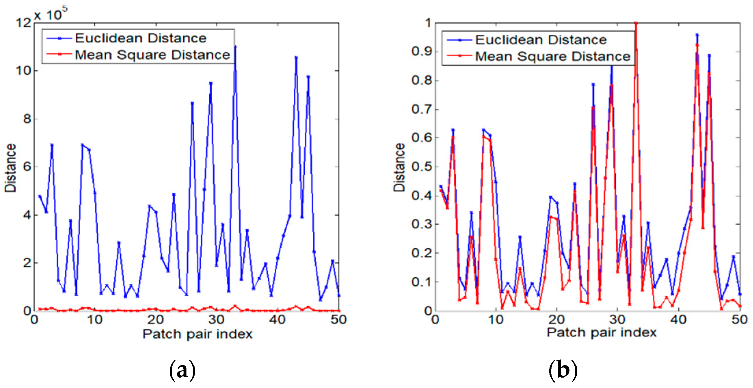
• We determine the MSD of image patches, and prove that it is more accurate than the Euclidean distance and can be expressed as the mean and std of the patches;
• We propose a pixel-level method to select similar pixels for fast NLE based on the 2D statistical histogram and summed area table;
• We propose to correct the initial estimation results by re-injecting noise to achieve more accurate NLE.

The rest of this paper is organized as follows. In Section 2, we propose our fast NLE method. We give the estimation and denoising results in Section 3. Finally, we conclude this paper in Section 4.

2. The Proposed Method

The generalized additive Gaussian white noise (AWGN) model can be formulated as $\mathit{y}=\mathit{x}+\mathit{n}$, where $\mathit{y}$ is the observed noisy image, $\mathit{x}$ is the original clean image, $\mathit{n}$ is the damaged noise and obeys the Gaussian independent identical distribution (i.i.d) $\mathit{n}~N(0,{\sigma }^2)$, and $\sigma$ is the standard deviation (std) of noise. Furthermore, $\sigma$ is also the noise level parameter to be focused on during estimation, as expanded on below.

2.1. Mean Square Distance

To solve the time-consuming problem caused by searching for similar patches and pixels, we express the MSD as the std and mean of the image patch.

Suppose the noisy image $\mathit{y}$ contains $N$ image patches {${\mathit{y}}_v$}$\in {\mathbb{R}}^{\sqrt{n}\times \sqrt{n}}(v=\mathrm{1,2},\dots ,N)$ of size $\sqrt{n}\times \sqrt{n}$; considering a reference image patch, ${\mathit{y}}_u$ ($u=\mathrm{1,2},\dots ,N$), in order to search a sufficient number of similar patches, for any image patch, ${\mathit{y}}_v$, to be searched for, we express the MSD as follows:

$$\begin{gathered} d_{uv}={‖{\mathit{y}}_u-{\mathit{y}}_v‖}_2=E\left\{{\left({\mathit{y}}_u-{\mathit{y}}_v\right)}^2\right\} \\ =E\left\{{\left[{\mathit{y}}_u-E\left({\mathit{y}}_u\right)-{\mathit{y}}_v+E\left({\mathit{y}}_v\right)+E\left({\mathit{y}}_u\right)-E\left({\mathit{y}}_v\right)\right]}^2\right\} \\ \triangleq {\left({\mu }_u-{\mu }_v\right)}^2+{\sigma }_u^2+{\sigma }_v^2-2cov\left({\mathit{y}}_u,{\mathit{y}}_v\right) , \end{gathered}$$

(1)

where ${\mu }_u$ and ${\sigma }_u^2$ are the mean and variance of ${\mathit{y}}_u$ (${\mathit{y}}_v$ is the same), respectively. $cov({\mathit{y}}_u,{\mathit{y}}_v)$ is the covariance of ${\mathit{y}}_u$ and ${\mathit{y}}_v$. Notice the following statistical relationship,

$$\begin{gathered} cov\left({\mathit{y}}_u,{\mathit{y}}_v\right)=E\left\{\left[{\mathit{y}}_u-{\mu }_u\right]\left[{\mathit{y}}_v-{\mu }_v\right]\right\} \\ \hspace{0.17em} ={\mu }_{uv}-2{\mu }_u{\mu }_v+{\mu }_u{\mu }_v \\ ={\mu }_{uv}-{\mu }_u{\mu }_v, \end{gathered}$$

(2)

where ${\mu }_{uv}$ is the mean of the product of ${\mathit{y}}_u$ and ${\mathit{y}}_v$. Replacing Equation (2) and the correlation coefficient equation ${\eta }_{uv}=cov\left({\mathit{y}}_u,{\mathit{y}}_v\right)/\sqrt{{\sigma }_u{\sigma }_v}$ into Equation (1), we derive the following:

$$d_{uv}{=\left({\mu }_u-{\mu }_v\right)}^2+{\left({\sigma }_u-{\eta }_{uv}{\sigma }_v\right)}^2+(1-{\eta }_{uv}^2){\sigma }_u^2,$$

(3)

The patches most similar to reference patch ${\mathit{y}}_u$ are those with the features ${\mu }_u={\mu }_v$ and ${\sigma }_u={\sigma }_v$. Therefore, similar patches could be completely found using their statistical features, i.e., their mean and std. Unlike ${\mu }_{uv}$, ${\mu }_v$ and ${\sigma }_v$ can be independently computed and stored. However, ${\mu }_{uv}$ is also an indicator of patch similarity. To express ${\mu }_{uv}$ in the form of union ${\mu }_u$, ${\mu }_v$, and ${\sigma }_u$, ${\sigma }_v$, we give the following theorem, Theorem 1, by considering the quasi-Gaussian property [27,28,29] of noisy patches:

Theorem 1. 

Assuming that the noisy image patches ${\mathit{y}}_u$ and ${\mathit{y}}_v$ can be fitted via Gaussian distribution and approximately obey the Gaussian distributions ${\mathit{y}}_u~N_u({\mu }_u,{\sigma }_u^2)$ and ${\mathit{y}}_v~N_v({\mu }_v,{\sigma }_v^2)$, respectively, ${\mathit{y}}_u{\mathit{y}}_v$ obeys the Gaussian distribution ${\mathit{y}}_u{\mathit{y}}_v~N_{uv}({\mu }_{uv},{\sigma }_{uv}^2)$, where

$${\mu }_{uv}=\frac{{\mu }_u{\sigma }_v^2+{\mu }_v{\sigma }_u^2}{{\sigma }_u^2+{\sigma }_v^2}, {\sigma }_{uv}^2=\frac{{\sigma }_u^2{\sigma }_v^2}{{\sigma }_u^2+{\sigma }_v^2}$$

(4)

The detailed proof of Theorem 1 is as follows:

Proof of Theorem 1. 

The key of Theorem 1 is that the product of two Gaussian functions is still a Gaussian function. According to the assumption, the probability density functions (PDFs) of ${\mathit{y}}_u$ and ${\mathit{y}}_v$ are as follows:

$${\mathit{y}}_u=\frac{1}{\sqrt{2\pi }{\sigma }_u}exp(-\frac{{(y-{\mu }_u)}^2}{2{\sigma }_u^2})$$

$${\mathit{y}}_v=\frac{1}{\sqrt{2\pi }{\sigma }_v}exp(-\frac{{(y-{\mu }_v)}^2}{2{\sigma }_v^2})$$

Their product is as follows:

$$h(y)={\mathit{y}}_u{\mathit{y}}_v=\frac{1}{2\pi {\sigma }_u{\sigma }_v}exp[-\left(\frac{{(y-{\mu }_u)}^2}{2{\sigma }_u^2}+\frac{{(y-{\mu }_v)}^2}{2{\sigma }_v^2}\right)]$$

Consider the exponential part, and expand it into the quadratic function form of $y$:

$$\begin{gathered} \beta =\frac{{(y-{\mu }_u)}^2}{2{\sigma }_u^2}+\frac{{(y-{\mu }_v)}^2}{2{\sigma }_v^2} \\ =\frac{\left({\sigma }_u^2+{\sigma }_v^2\right)y^2-2\left({\mu }_u{\sigma }_v^2+{\mu }_v{\sigma }_u^2\right)y+{\mu }_u^2{\sigma }_v^2+{\mu }_v^2{\sigma }_u^2}{2{\sigma }_u^2{\sigma }_v^2} \end{gathered}$$

Compare eqn. $\beta$ with the ordinary Gaussian form:

$$P\left(y\right)=\frac{1}{\sqrt{2\pi }\sigma }exp(-\frac{{(y-\mu )}^2}{2{\sigma }^2})=\frac{1}{\sqrt{2\pi }\sigma }exp(-\frac{y^2-2\mu y+{\mu }^2}{2{\sigma }^2})$$

Formulate eqn. $\beta$ into the form of the ordinary Gaussian function:

$$\begin{gathered} \beta =\frac{y^2-2y\frac{{\mu }_u{\sigma }_v^2+{\mu }_v{\sigma }_u^2}{{\sigma }_u^2+{\sigma }_v^2}+{(\frac{{\mu }_u{\sigma }_v^2+{\mu }_v{\sigma }_u^2}{{\sigma }_u^2+{\sigma }_v^2})}^2}{2\frac{{\sigma }_u^2{\sigma }_v^2}{{\sigma }_u^2+{\sigma }_v^2}}+\frac{\frac{{\mu }_u{\sigma }_v^2+{\mu }_v{\sigma }_u^2}{{\sigma }_u^2+{\sigma }_v^2}-{(\frac{{\mu }_u{\sigma }_v^2+{\mu }_v{\sigma }_u^2}{{\sigma }_u^2+{\sigma }_v^2})}^2}{2\frac{{\sigma }_u^2{\sigma }_v^2}{{\sigma }_u^2+{\sigma }_v^2}} \\ =\frac{{(y-\frac{{\mu }_u{\sigma }_v^2+{\mu }_v{\sigma }_u^2}{{\sigma }_u^2+{\sigma }_v^2})}^2}{2\frac{{\sigma }_u^2{\sigma }_v^2}{{\sigma }_u^2+{\sigma }_v^2}}+\frac{{({\mu }_u-{\mu }_v)}^2}{2({\sigma }_u^2+{\sigma }_v^2)} \end{gathered}$$

Let ${\sigma }_{uv}^2=\frac{{\sigma }_u^2{\sigma }_v^2}{{\sigma }_u^2+{\sigma }_v^2}$, ${\mu }_{uv}=\frac{{\mu }_u{\sigma }_v^2+{\mu }_v{\sigma }_u^2}{{\sigma }_u^2+{\sigma }_v^2}$, then

$$\beta =\frac{{(y-{\mu }_{uv})}^2}{2{\sigma }_{uv}}+\frac{{({\mu }_u-{\mu }_v)}^2}{2({\sigma }_u^2+{\sigma }_v^2)}$$

Substitute this into Eqn. $h\left(y\right)$ to obtain the following:

$$h\left(y\right)=\frac{1}{\sqrt{2\pi }{\sigma }_{uv}}exp(-\frac{{(y-{\mu }_{uv})}^2}{2{\sigma }_{uv}^2})\frac{1}{\sqrt{2\pi ({\sigma }_u^2+{\sigma }_v^2)}}exp(-\frac{{({\mu }_u-{\mu }_v)}^2}{2({\sigma }_u^2+{\sigma }_v^2)})$$

Therefore, when normalization can be ignored, this is enough to prove that $h\left(y\right)$ is a Gaussian function,

$$h\left(y\right)=\frac{G_{uv}}{\sqrt{2\pi }{\sigma }_{uv}}exp(-\frac{{(y-{\mu }_{uv})}^2}{2{\sigma }_{uv}^2})$$

where the scaling factor, $G_{uv}$, is itself a gaussian probability density function (PDF) on mean ${\mu }_v$ with the standard deviation $\sqrt{{\sigma }_u^2+{\sigma }_v^2}$

$$G_{uv}=\frac{1}{\sqrt{2\pi ({\sigma }_u^2+{\sigma }_v^2)}}exp(-\frac{{({\mu }_u-{\mu }_v)}^2}{2({\sigma }_u^2+{\sigma }_v^2)})$$

In other words, the distribution function of the product is a compressed or amplified Gaussian distribution. $G_{uv}$ is the scaling factor, and the integral of the probability density of the product is not equal to 1, but its variance and mean value properties remain unchanged. □

According to Theorem 1, ${\mu }_{uv}$ can be expressed by the mean value ${\mu }_u$, ${\mu }_v$ and standard deviation ${\sigma }_u$, ${\sigma }_v$ of ${\mathit{y}}_u$ and ${\mathit{y}}_v$. It should be noted that the condition of Theorem 1 is that both ${\mathit{y}}_u$ and ${\mathit{y}}_v$ approximately obey the Gaussian distribution, while non-homogeneous noisy image patches are not necessarily true. Therefore, this paper is only used to replace ${\mu }_{uv}$ approximately. In this approximation, Equation (3) is transformed into the following:

$$d_{uv}={\mu }_u^2+{\mu }_v^2+{\sigma }_u^2+{\sigma }_v^2-2\frac{{\mu }_u{\sigma }_v^2+{\mu }_v{\sigma }_u^2}{{\sigma }_u^2+{\sigma }_v^2}$$

(5)

Now, the similarity of two patches can be calculated using the new distance, i.e., the MSD, and it is only related to the mean and standard deviation of the statistical characteristics of patches. Obviously, the problem of finding similar patches is the use of a search strategy.

From Figure 1, it can be seen that the actual MSD is at least two orders of magnitude smaller than the Euclidean distance. After normalization (i.e., dividing all data by the maximum value), the two trends are basically the same, and the Euclidean distance is more sensitive to data, especially noise; only by increasing the distance threshold can enough similar patches be selected. Increasing the threshold has a significant impact on the selection of different regions; the MSD is more robust in selecting similar patches. Therefore, we can search for a similar mean and std to obtain similar patches. In the following sub-section, a 2D histogram and summed area table are provided for the fast searching of similar patches.

2.2. Image Patch Feature Statistics

2.2.1. 2D Statistical Histogram to Represent Statistical Features

For the image patch set {${\mathit{y}}_v$}$\in {\mathbb{R}}^{\sqrt{n}\times \sqrt{n}}(v=\mathrm{1,2},\dots ,N)$, we can obtain the mean, ${\mu }_v$, and the std, ${\sigma }_v$, for each patch, ${\mathit{y}}_v$. Let $N_{\mu }$, $N_{\sigma }$ represent the total bins in ${\mu }_v$ and ${\sigma }_v$, respectively; the variables ${\mu }_v$ and ${\sigma }_v$ can be correlated using the 2D statistical histogram $H\left(\mu ,\sigma \right)\in {\mathbb{R}}^{N_{{\mu }_v}\times N_{{\sigma }_v}}$ shown in Figure 2b. For example, $H\left({\mu }_1,{\sigma }_2\right)$ indicates the number that satisfies $\mu ={\mu }_1$ and $\sigma ={\sigma }_2$ simultaneously. The 2D statistical histogram directly reveals the distribution of patch features.

2.2.2. Summed Area Table for Fast Calculation of the Number of Similar Patches

For a reference patch, ${\mathit{y}}_{\mathit{u}}$, the number of similar patches can be found the from 2D statistical histogram directly. Considering that there will be a large number of similar patches in homogeneous regions, such as the “sky” region in Figure 2a, the number of patches with special texture is very small. If few similar patches are found, searching for sufficiently similar patches in the whole feature domain iteratively is time-consuming. To solve this problem, the summed area table [25] is employed to improve search speed.

A summed area table, denoted $SAT(x,y)$, represents the sum of values located in the upper-left rectangular region of location $H[x,y]$, which is defined as follows [25]:

$$SAT(x,y)=\sum _{x^{\prime }\le x,y^{\prime }\le y}H[x^{\prime },y^{\prime }]$$

(6)

where x and y represent the coordinates in the 2D statistical histogram, and $x^{\prime }$ and $y^{\prime }$ represent coordinates smaller than x and y, respectively. As shown in Figure 3, the sum of a rectangular region can be easily obtained via

$$\sum _{\begin{array}{c}{L_1\left(x\right)\le x}^{\prime }\le L_4\left(x\right)\\ L_1\left(y\right){\le y}^{\prime }\le L_4\left(y\right)\end{array}}H[x^{\prime },y^{\prime }]=L_4+L_1-L_2-L_3$$

(7)

where $L_1$, $L_2$, $L_3$, and $L_4$ are the four angular coordinates of the sum of the rectangular regions. For simplicity, the coordinate variables $x^{\prime }$ and $y^{\prime }$ are hidden. The 2D histogram counts the mean, variance, and coordinates of all patches in the image. Assuming that the current patch’s mean and variance are (${\mu }_1,{\sigma }_2$), i.e., $(x,y)$ in Equation (6), if the patch is in a smooth region, there are many similar patches. We can search and calculate a sufficient number of similar patches only at and near (${\mu }_1,{\sigma }_2$) in the 2D histogram. At this point, the difference in time consumption between directly searching, calculating, and using $SAT$ is small. If the patch is located in a special texture region, such as corners or other regions with fast texture changes, there are fewer similar patches. We need to search and calculate the number of patches in (${\mu }_1,{\sigma }_2$) and larger areas of the 2D histogram while $SAT$ stores the cumulative number of patches’ mean and variance in different positions in advance. By setting search ranges $L_1$, $L_2$, $L_3$, and $L_4$ for the mean and variance (${\mu }_1,{\sigma }_2$), $SAT$ can quickly calculate the required number without the need for an iterative search and calculation. It is seen from Equation (7) that the search for similar patches using the summed-area table involves only three addition and subtraction operations.

2.3. Similar Patch and Pixel Search

We only need a mean filter and an std filter to quickly obtain the mean and std of all patches in noisy images. The 2D statistical histogram is used to count these mean and std values, the summed area table is used to quickly search for enough similar patches, and the MSD is used to find the most similar patches. The search strategies for similar patches and pixels in this paper are as follows.

Horizontal Search for Similar Patches. Suppose we want to search for $m$ patches, ${\mathit{Y}}_u=[{\mathit{y}}_{v,1},{\mathit{y}}_{v,2},\dots ,{\mathit{y}}_{v,m}]\in {\mathbb{R}}^{\sqrt{n}\times \sqrt{n}}$ (including ${\mathit{y}}_u$ itself, i.e., ${\mathit{y}}_u={\mathit{y}}_{v,1}$), that are most similar to ${\mathit{y}}_u$ from the patch set {${\mathit{y}}_v$}$\in {\mathbb{R}}^{\sqrt{n}\times \sqrt{n}}$ $(v=\mathrm{1,2},\dots ,N)$; we give priority to the case where the mean is equal, i.e., ${\mu }_u={\mu }_v$, and then gradually increase and decrease the std to search for similar patches. If the number of patches is insufficient, we only need to increase the search and calculation ranges of ${\mu }_u$ and ${\sigma }_u$, i.e., $L_1$, $L_2$, $L_3$, and $L_4$, to quickly find enough similar patches. The summed area table is used to calculate the number of similar patches to speed up the search, i.e., $m=SAT(x,y)$. It should be noted that such a similar patch search strategy is global for the original image in a feature domain, i.e., with the mean and std.

The formation of ${\mathit{Y}}_u$ is based on the similarity of the patch level, and we call this the horizontal search for similar patches. For the similarity of two patches, priority is given to ensuring that the pixels in the same row are similar to some extent. However, for rare image textures and details, some pixels will have large changes due to changes in shape. The similarity of these pixels at the same level is not reasonable. In order to solve this problem, we stretch the patches in ${\mathit{Y}}_u=[{\mathit{y}}_{v,1},{\mathit{y}}_{v,2},\dots ,{\mathit{y}}_{v,m}]\in {\mathbb{R}}^{\sqrt{n}\times \sqrt{n}}$ into vector ${\mathit{I}}_u=[{\mathit{I}}_{v,1},{\mathit{I}}_{v,2},\dots ,{\mathit{I}}_{v,m}]\in {\mathbb{R}}^{1\times n}$ by column and carefully select the most similar pixels from ${\mathit{I}}_u$.

Vertical Search for Similar Pixels. For each row of ${\mathit{I}}_u$, there are $m$ pixels in the same location of different patches that are similar to each other. In order to refine the similarity of pixels, consider the $i$-th row in ${\mathit{I}}_u$, i.e., ${\mathit{I}}_v^i$, and calculate the distance, $d_v^{ij}={‖{\mathit{I}}_v^i-{\mathit{I}}_v^j‖}_2$, between the $i$-th row, ${\mathit{I}}_v^i$, and the $j$-th row, ${\mathit{I}}_v^j$. Finally, select the $q$ rows, {${\mathit{I}}_v^{i_1},{\mathit{I}}_v^{i_2},\dots ,{\mathit{I}}_v^{i_q}$}, which are most similar to those of ${\mathit{I}}_v^i$ (including ${\mathit{I}}_v^i$ itself), and aggregate these rows into the matrix ${\mathit{{\rm I}}}_u^{i_q}{\in \mathbb{R}}^{q\times m}$,

$${\mathit{{\rm I}}}_u^{iq}=\left[\begin{array}{ccc}{I}_v^{i_1,1}& \cdots & I_v^{i_1,m}\\ ⋮& \ddots & ⋮\\ I_v^{i_{\mathrm{q}},1}& \cdots & I_v^{i_{\mathrm{q}},m}\end{array}\right]$$

(8)

where {$i_1,i_2,\dots ,i_{\mathrm{q}}$}$\subset \{\mathrm{1,2},\dots ,n\}$. For each row ${\mathit{I}}_v^i$ of ${\mathit{I}}_u$, the most similar pixel matrix, ${\mathit{{\rm I}}}_u^{iq}$, of $q$ rows can be searched for. Traversing all rows of ${\mathit{I}}_u$ to obtain the set, {${\mathit{{\rm I}}}_u^{iq}$}($i=\mathrm{1,2},\dots ,n; u=\mathrm{1,2},\dots ,N$), of similar pixels in different regions of the entire image, we can estimate the noise level of the image according to each ${\mathit{{\rm I}}}_u^{iq}$, because each ${\mathit{{\rm I}}}_u^{iq}$ is composed of the most similar rows.

2.4. Noise Level Estimation

Since the pixels in the selected $q$ rows of ${\mathit{{\rm I}}}_v^{iq}$ are very similar to each other, the authors of [2] explained that this similar pixel search scheme can convert non-Gaussian real noise into quasi-Gaussian noise; therefore, the std of among them can be viewed as the noise level. For simplicity, we assume that the noise follows a Gaussian distribution with std $\sigma$. Let the distances between the $i$-th row of ${\mathit{I}}_v$ and its most similar $q$ rows be $d_v^{i{i}_1},d_v^{i{i}_2},\dots ,d_v^{i{i}_q}$($i_1=i$); the local noise level (LNL) ${\sigma }_u$ of this paper can be computed as follows:

$${\sigma }_u=\frac{1}{n(q-1)}\sum _{t=2}^q\sum _{i=1}^n\sqrt{\frac{1}{m}{\left(d_v^{i{i}_t}\right)}^2}$$

(9)

In NLE-NSS [2], the strategy of searching for similar patches based on the neighborhood makes it easy to select less similar patches when the distribution of similar textures is very scattered, which leads to an overestimation of the local noise level. However, our method of searching for similar patches based on the feature domain is global and can be used for the pixel domain; thus, the proposed method is more feasible than the method in [2].

On the other hand, in order to make the proposed method more robust for NLE without overestimation, we extend the NLE from a local region to a global one. To achieve this, the initial global noise level (GNL) is averaged by the local estimated ${\sigma }_u$ as follows:

$${\sigma }_g=\frac{1}{N}\sum _{v=1}^N{\sigma }_u$$

(10)

In addition, the image content might magnify or attenuate the noise effects to some extent. Although our method obtains a good estimation result, the preliminary experimental results in Figure 4 show that our estimation has a bias, and the relationship between our estimate and the true noise level is approximately linear. To further reduce estimation bias, we suggest a rectification procedure based on noise injection.

Specifically, we formulate the relationship between the initial estimation, ${\sigma }_g$, and the underlying true noise level, $\sigma$, using the following linear model:

$${\sigma }_g=\alpha \sigma$$

(11)

Clearly, there are two unknown variables, $\mathsf{\alpha }$ and $\sigma$, in (11). Uncovering these two unknowns from a single equation is an ill-posed problem. To tackle this challenge, we employ noise injection strategy to generate an additional equation. We inject the same type of i.i.d. noise with variance ${\sigma }_t^2$ into the noisy image, and carry out an additional round of noise estimation. Due to the independence between the original noise and the injected noise, we have

$$\left\{\begin{array}{c}{\sigma }_{g,1}^2={\alpha }^2{\sigma }^2,\\ {\sigma }_{g,2}^2={\alpha }^2{(\sigma }^2+{\sigma }_t^2)\end{array}\right.$$

(12)

where ${\sigma }_{g,1}^2$ and ${\sigma }_{g,2}^2$ denote the estimated noise variances before and after injection, respectively. Here, the value of $\alpha$ is assumed to be invariant in those two rounds of NLE. This assumption is reasonable because $\alpha$ only depends on the original image content; as shown in Figure 4, even if the noise level increases after secondary injection of noise, the estimated deviation still satisfies Figure 4a while the original image remains unchanged. Therefore, we fixed $\alpha$. From (12), it is easy to solve ${\sigma }^2$ as follows:

$${\sigma }^2=\frac{{\sigma }_{g,1}^2{\sigma }_t^2}{{\sigma }_{g,2}^2-{\sigma }_{g,1}^2}$$

(13)

Conceptually, the variance in injected noise can be set arbitrarily. However, too heavy an injection tends to wipe out the effects resulting from the image content in practice. One reasonable choice is to set the injected noise variance as the first estimated one, i.e., ${\sigma }_t^2={\sigma }_{g,1}^2$. Note that the noise level becomes larger after noise injection, which implies ${\sigma }_{g,2}^2>{\sigma }_{g,1}^2$. Then, the underlying true noise variance can be estimated via the following:

$${\widehat{\sigma }}_g^2=\frac{{\sigma }_{g,1}^4}{{\sigma }_{g,2}^2-{\sigma }_{g,1}^2}$$

(14)

However, due to the simplicity of this linear model, the rectified noise level may still slightly deviate from the true noise level. To make a more robust estimation, we fuse the estimated results before and after noise injection together through a linear convex combination,

$$\widehat{\sigma }=\sqrt{{\beta }_0{\widehat{\sigma }}_g^2+{\beta }_1{\sigma }_g^2}$$

(15)

where $\widehat{\sigma }$ denotes the final estimation, and ${\beta }_0$ and ${\beta }_1$ are weighting factors satisfying ${\beta }_0+{\beta }_1=1$. In our proposed scheme, ${\beta }_0$= 0.613 and ${\beta }_1$= 0.387, which are obtained from an off-line training procedure with over 100 noisy images in the BSDS500 [30] benchmark dataset.

2.5. Algorithm and Complexity Analysis

The proposed method is summarized as follows, as Algorithm 1:

Algorithm 1 Estimating Noise Level

Inputs: $\mathrm{Observed} \mathrm{image} \mathit{y}\in {\mathbb{R}}^{h\times w}$$, \mathrm{and} \mathrm{parameters} \sqrt{n}$$, m$$, q$ $1: \mathrm{The} \mathrm{mean} \mathrm{filter} MEAN(\mathit{y},[\sqrt{n},\sqrt{n}\left]\right)$$\mathrm{and} \mathrm{std} \mathrm{filter} STD(\mathit{y},[\sqrt{n},\sqrt{n}\left]\right)$ are used to   $\mathrm{calculate} \mathrm{the} \mathrm{mean} \mu$$\mathrm{and} \mathrm{std} \sigma$ of each patch $2: 2\mathrm{D} \mathrm{histogram} H\left(\mu ,\sigma \right)$$\mathrm{statistics} \mu$$\mathrm{and} \sigma$ $3: \mathbf{for} u=1:v$   $\mathrm{Search} m$$\mathrm{most} \mathrm{similar} \mathrm{patches} \mathrm{and} \mathrm{stretch} \mathrm{into} \mathrm{vector} {\mathit{I}}_u$$\mathrm{by} \mathrm{use} \mathrm{summed-area} \mathrm{table} SAT(x,y)$$\mathrm{in} H\left(\mu ,\sigma \right)$   Calculate the most similar $q$ rows of each row to obtain $\left\{{\mathit{{\rm I}}}_u^{iq}\right\}$   Calculate the local noise level ${\sigma }_u$$\mathrm{from} \left\{{\mathit{{\rm I}}}_u^{iq}\right\}$   end for $4: \mathrm{Obtain} \mathrm{the} \mathrm{initial} \mathrm{estimation} {\sigma }_g$$\mathrm{from} \mathrm{all} \mathrm{local} \mathrm{noise} \mathrm{level} {\sigma }_u$ $5: \mathbf{return} \mathrm{the} \mathrm{final} \mathrm{estimate} \widehat{\sigma }$ is obtained by Equations (14) and (15) with quadratic estimation correction

We gradually analyze the complexity of the proposed algorithm as follows:

(1)

The complexity of calculating patch mean ${\mu }_v$, std ${\sigma }_v$ is $\mathcal{O}$($N$), establishing 2D statistical histogram $H\left(\mu ,\sigma \right)$ is $\mathcal{O}$($N$);

(2)

The complexity of searching similar patches is $\mathcal{O}$($rN$), where $r$ is the number of times to gradually increase or decrease the mean and std;

(3)

The complexity of searching similar pixels is $\mathcal{O}$($n^{2}rN$);

(4)

The complexity of computing ${\sigma }_u$ is $\mathcal{O}$($N$), the complexity of computing ${\sigma }_g$, $\widehat{\sigma }$, and each calculation of the summed-area table $SAT(x,y)$ is $\mathcal{O}$(1).

In summary, NLE is performed twice, and the algorithm complexity of the proposed method is $\mathcal{O}$(${2n}^{2}rN$). Compared with the most relevant method [2], each calculation of the local noise level in the method in [2] needs to search for similar patches in the neighborhood with the size of $W\times W$, and the overall complexity of the method in [2] is $\mathcal{O}$(${nW}^{2}N$). Meanwhile, the proposed method only needs to increase or decrease the mean and std every time. Our experiments show that we can search for a sufficient number of similar patches only by increasing or decreasing them a few times, i.e., $W>n\gg r$. Therefore, the proposed method is more efficient than the method in [2].

3. Experimental Results

To evaluate the performance of the proposed fast NLE (FNLE) method, we compare our FNLE method with seven state-of-the-art methods: Liu’s method [14], Wu’s method [19], Yang’s methods [12], Zoran’s method [15], the PCA method [20], Hou’s method [2], and Gupta’s method [17]. For a fair comparison, all the methods are implemented by using Matlab R2014a on a laptop with Windows 10 OS, with 8G RAM, 2.4 GHz CPU, and Intel Core i5-6300U. The parameters of our FNLE are set as follows: the image patch size is $\sqrt{n}$ = 7, the minimum number of similar patches is $m=64$, and the number of rows for similar pixels is $q=8$.

Furthermore, we consider two benchmark datasets: TID2008 [26] and BSDS500 [30]. The TID2008 dataset [26] has been widely used for the evaluation of full-reference image quality assessment metrics, which contain 25 reference images without any compression, but it has been argued that all images in the TID2008 dataset contain small or large homogeneous regions [24]. To further demonstrate the robustness of our method on images full of textures, we compare the performance of different methods on a more challenging dataset—the BSDS500 dataset with 200 test images [30]. All images are injected with additive Gaussian white noise (AWGN) at different noise levels, $\sigma =\{1, 3, 5, 10, 20, 30, 40, 50\}$, i.e., all pixels of images are polluted by noise. Different methods are used to estimate the noise levels of noisy images.

To further evaluate the performance of the proposed method on real noisy images, two benchmark datasets of real-world images are considered: the Cross-Channel (CC) dataset [31] and the Darmstadt Noise Dataset (DND) [32].

The CC dataset [31] includes noisy images of 11 static scenes captured by Canon 5D Mark 3, Nikon D600, and Nikon D800 cameras. The real-world noisy images were collected under a controlled indoor environment. Each scene was shot 500 times using the same camera and settings. The average of the 500 shots is taken as the “ground truth”. The authors cropped 15 images measuring a size of 512 × 512 to evaluate different NLE methods.

The DND dataset [32] includes 50 different scenes captured by Sony A7R, Olympus E-M10, Sony RX100 IV, and Huawei Nexus 6P. Each scene contains a pair of noisy and “ground truth” clean images. The noisy images are collected under higher ISO values with shorter exposure times, while the “ground truth” images are captured under lower ISO values with longer adjusted exposure times. For each scene, the authors cropped 100 bounding boxes measuring a size of 512 × 512 to evaluate different NLE methods.

With the “ground truth” and noisy images, the truth noise variance can be easily calculated according to the difference between the two images. As [19] estimates the noise level for each channel separately when handling colorful images, NLE is finally achieved by averaging the NLE of each channel. Evaluation indicators include the mean (Mean), the standard deviation (Std) and the root mean square error (RMSE) of the estimated results. The “Mean” is used to evaluate the accuracy of an estimator, “Std” is used to evaluate the robustness of an estimator, and “RMSE” is used to evaluate the overall performance of an estimator. Note that the smaller the bias, STD, or RMSE is, the better the estimator is.

Table 1. Comparison of AWGN estimation results. The best results are highlighted in bold.

Noise Level		Liu [14]		Wu [19]		Yang [12]		Zoran [15]		Pyatykh [20]		Hou [2]		Gupta [17]		FNLE
		Mean	Std	Mean	Std	Mean	Std	Mean	Std	Mean	Std	Mean	Std	Mean	Std	Mean	Std
BSDS 500	1	0.99	0.25	1.39	0.32	2.05	1.33	0.72	1.59	1.25	0.53	3.89	1.53	3.00	1.70	1.44	0.48
	3	2.84	0.26	3.14	0.28	3.75	1.03	2.77	1.46	3.16	0.31	5.05	0.62	4.05	1.30	3.14	0.32
	5	4.91	0.14	5.07	0.14	5.61	0.86	4.67	1.38	5.15	0.21	5.91	0.73	5.66	1.10	5.07	0.18
	10	9.92	0.18	10.07	0.10	10.43	0.63	9.56	1.25	10.13	0.17	10.52	0.62	9.89	1.71	10.06	0.10
	20	19.91	0.21	20.04	0.09	20.24	0.44	19.31	1.32	20.09	0.35	20.54	0.73	19.80	0.32	20.01	0.09
	30	29.82	0.26	30.05	0.21	30.15	0.40	29.18	1.38	29.82	0.50	30.67	0.54	29.50	0.28	30.04	0.21
	40	39.70	0.27	40.09	0.29	40.17	0.52	39.09	1.39	39.47	0.69	40.71	0.75	39.22	0.26	40.07	0.25
	50	49.53	0.32	50.27	0.32	49.87	0.60	49.06	1.43	49.14	0.83	50.49	0.69	48.74	0.29	49.92	0.28
TID 2008	1	3.08	3.31	1.43	0.45	2.11	0.90	1.99	1.29	1.43	0.54	2.84	1.33	3.07	3.30	1.84	0.71
	3	4.43	2.92	3.27	0.27	3.71	0.70	3.53	1.68	3.31	0.35	3.98	1.01	4.42	2.92	3.26	0.41
	5	6.02	2.64	5.14	0.40	5.56	0.60	4.25	1.61	5.14	0.31	5.92	0.92	6.01	2.64	5.13	0.33
	10	10.49	2.03	10.04	0.11	10.38	0.46	9.09	2.12	10.12	0.10	10.73	0.83	10.49	2.03	10.03	0.09
	20	19.98	1.32	20.01	0.14	20.22	0.37	19.15	1.78	19.97	0.27	20.69	0.85	19.98	1.32	20.01	0.14
	30	29.56	0.97	30.08	0.15	30.07	0.36	28.82	1.14	29.78	0.59	30.64	0.79	29.56	0.97	30.06	0.14
	40	39.23	0.77	40.22	0.31	39.81	0.45	38.77	1.16	39.44	0.72	40.50	0.61	39.23	0.77	40.16	0.29
	50	48.85	0.67	50.39	0.47	49.70	0.52	48.72	1.14	49.20	0.77	50.44	0.55	48.81	0.67	50.33	0.32

and Figure 5a,b show the results of the estimation of synthetic noise via various methods, and Figure 5c,d show the results of the estimation of real-world noise images. It can be seen from Table 1 and Figure 5a–d that the proposed FNLE method is slightly inferior to Liu’s and Wu’s methods when the noise is 1–5 but better than other methods in other cases.

Image denoising is a very important preliminary step for many computer vision methods. During the past few decades, impressive improvements have been made in this area. However, the noise level, $\sigma$, is regarded as a known parameter in many algorithms with good performance. BM3D [1] is one of such algorithms that requires the noise level as an input parameter. We apply our NLE method to guide the BM3D image denoising algorithm. In addition, we choose the peak signal-to-noise ratio ($PSNR$) and $SSIM$ as evaluation indexes. Note that the larger the $PSNR$ or $SSIM$, the better the denoising performance.

Table 2. Average results of PSNR, SSIM, and execution time (seconds) obtained via guided BM3D denoising with different methods of estimating real-world noise images in the CC dataset [31] and DND dataset [32]. The best results are highlighted in bold.

-	-	Noisy Image	Liu [14]	Wu [19]	Yang [12]	Zoran [15]	Pyatykh [20]	Hou [2]	Gupta [17]	FNLE
CC dataset	PSNR	33.41	33.58	35.68	33.56	33.61	33.45	33.82	34.75	35.76
	SSIM	0.9079	0.9114	0.9474	0.9113	0.912	0.9087	0.9161	0.9258	0.9491
	Time	-	5.767	2.669	2.435	12.628	19.783	3.027	314.012	1.277
DND dataset	PSNR	28.81	28.86	33.38	31.50	29.01	31.31	30.26	31.69	33.57
	SSIM	0.7893	0.7917	0.9166	0.8743	0.7974	0.8711	0.8642	0.8892	0.9201
	Time	-	3.086	2.386	2.272	10.358	17.472	2.994	301.868	1.242

shows the PSNR and SSIM results of BM3D denoising guided by the noise level estimations of different algorithms in the CC dataset and DND dataset. It can be seen from the Table 2 that the proposed FNLE estimates the real-world noise image more accurately, has better denoising performance, and obtains higher PSNR and SSIM values. Therefore, the proposed FNLE method is more suitable than other methods for estimating real-world noise images. In addition, without the optimized program, the proposed method achieves the highest operating efficiency.

In addition, Figure 6 and Figure 7 show the visual comparisons of the images denoised using BM3D with different noise level parameters. It can be seen that the proposed FNLE method achieves higher PSNR and SSIM values, with better visual quality than that of the other methods.

4. Conclusions

In order to overcome the influence of complex image texture on NLE, a fast image NLE method based on similar pixels is proposed in this paper. Specifically, the MSD is expressed as the std and mean of image patches. A 2D statistical histogram and summed area table are adopted to search for similar patches and pixels quickly. In particular, we extend the estimation from local to global and correct the deviation of the initial estimation. The experimental results show that the proposed method is superior to the state-of-the-art methods in terms of fast NLE and guided denoising. In particular, the proposed method is more suitable for NLE of real-world images.

References

1. Dabov, K.; Foi, A.; Katkovnik, V.; Egiazarian, K. Image denoising by sparse 3-D transform-domain collaborative filtering. IEEE Trans. Image Process. 2007, 16, 2080–2095. [Google Scholar] [CrossRef] [PubMed]
2. Hou, Y.; Xu, J.; Liu, M.; Liu, G.; Liu, L.; Zhu, F.; Shao, L. NLH: A Blind Pixel-Level Non-Local Method for Real-World Image Denoising. IEEE Trans. Image Process. 2020, 29, 5121–5135. [Google Scholar] [CrossRef]
3. Li, B.; Ng, T.T.; Li, X.; Tan, S.; Huang, J. Revealing the Trace of High-Quality JPEG Compression Through Quantization Noise Analysis. IEEE Trans. Inf. Forensics Secur. 2017, 10, 558–573. [Google Scholar]
4. Guo, F.F.; Wang, X.X.; Shen, J. Adaptive fuzzy c-means algorithm based on local noise detecting for image segmentation. IET Image Process. 2016, 10, 272–279. [Google Scholar] [CrossRef]
5. Jiang, P.; Zhang, J.-Z. No-reference image quality assessment based on local maximum gradient. J. Electron. Inf. Technol. 2015, 37, 2587–2593. [Google Scholar]
6. Scharr, H.; Spies, H. Accurate optical flow in noisy image sequences using flow adapted anisotropic diffusion. Signal Process. Image Commun. 2005, 20, 537–553. [Google Scholar] [CrossRef]
7. Nan, Y.; Quan, Y.; Ji, H. Variational-EM-Based Deep Learning for Noise-Blind Image Deblurring. In Proceedings of the IEEE Conference on Computer Vision and Pattern Recognition (CVPR), Seattle, WA, USA, 13–19 June 2020. [Google Scholar]
8. Heidari-Gorji, H.; Ebrahimpour, R.; Zabbah, S. A temporal hierarchical feedforward model explains both the time and the accuracy of object recognition. Sci. Rep. 2021, 11, 5640. [Google Scholar] [CrossRef] [PubMed]
9. Pratap, T.; Kokil, P. Efficient Network Selection for Computer-aided Cataract Diagnosis Under Noisy Environment. Comput. Methods Programs Biomed. 2021, 200, 105927. [Google Scholar] [CrossRef]
10. Gureyev, T.E.; Paganin, D.M.; Kozlov, A.; Nesterets, Y.I.; Quiney, H.M. Complementary aspects of spatial resolution and signal-to-noise ratio in computational imaging. Phys. Rev. A 2018, 97, 053819. [Google Scholar] [CrossRef]
11. Katase, H.; Yamaguchi, T.; Fujisawa, T.; Ikehara, M. Image noise level estimation by searching for smooth patches with discrete cosine transform. In Proceedings of the 2016 IEEE 59th International Midwest Symposium on Circuits and Systems (MWSCAS), Abu Dhabi, United Arab Emirates, 16–19 October 2016. [Google Scholar]
12. Yang, S.M.; Tai, S.C. Fast and reliable image-noise estimation using a hybrid approach. J. Electron. Imaging 2010, 19, 033007. [Google Scholar] [CrossRef]
13. Kokil, P.; Pratap, T. Additive white gaussian noise level estimation for natural images using linear scale-space features. Circuits Syst. Signal Process. 2021, 40, 353–374. [Google Scholar] [CrossRef]
14. Liu, X.; Tanaka, M.; Okutomi, M. Noise level estimation using weak textured patches of a single noisy image. In Proceedings of the IEEE International Conference on Image Processing, Orlando, FL, USA, 30 September–3 October 2012; pp. 665–668. [Google Scholar]
15. Zoran, D.; Weiss, Y. Scale invariance and noise in natural images. In Proceedings of the IEEE 12th International Conference on Computer Vision (ICCV), Kyoto, Japan, 29 September–2 October 2009; pp. 2209–2216. [Google Scholar]
16. Wu, M.W.; Jin, Y.; Li, Y.; Song, T.; Kam, P.Y. Maximum-Likelihood, Magnitude-Based, Amplitude and Noise Variance Estimation. IEEE Signal Process. Lett. 2021, 28, 414–418. [Google Scholar] [CrossRef]
17. Gupta, P.; Bampis, C.G.; Jin, Y.; Bovik, A.C. Natural scene statistics for noise estimation. In Proceedings of the 2018 IEEE Southwest Symposium on Image Analysis and Interpretation (SSIAI), Las Vegas, NV, USA, 8–10 April 2018. [Google Scholar]
18. Fang, Z.; Yi, X. A novel natural image noise level estimation based on flat patches and local statistics. Multimed. Tools Appl. 2019, 78, 17337–17358. [Google Scholar] [CrossRef]
19. Wu, J.X.; Xie, S.L.; Li, Z.G.; Wu, S.Q. Image noise level estimation via kurtosis test. J. Electron. Imaging 2022, 31, 033015. [Google Scholar] [CrossRef]
20. Pyatykh, S.; Hesser, J.; Zheng, L. Image noise level estimation by principal component analysis. IEEE Trans. Image Process. 2013, 22, 687–699. [Google Scholar] [CrossRef] [PubMed]
21. Jiang, P.; Wang, Q.; Wu, J. Efficient Noise-Level Estimation Based on Principal Image Texture. IEEE Trans. Circuits Syst. Video Technol. 2020, 30, 1987–1999. [Google Scholar] [CrossRef]
22. Liu, W.; Lin, W. Additive white Gaussian noise level estimation in SVD domain for images. IEEE Trans. Image Process. 2013, 22, 872–883. [Google Scholar] [CrossRef] [PubMed]
23. Tang, C.; Yang, X.; Zhai, G. Noise Estimation of Natural Images via Statistical Analysis and Noise Injection. IEEE Trans. Circuits Syst. Video Technol. 2015, 25, 1283–1294. [Google Scholar] [CrossRef]
24. Chen, G.; Zhu, F.; Heng, P.A. An efficient statistical method for image noise level estimation. In Proceedings of the IEEE International Conference on Computer Vision (ICCV), Santiago, Chile, 7–13 December 2015; pp. 477–485. [Google Scholar]
25. Crow, F. Summed-Area Tables for Texture Mapping; SIGGRAPH: Chicago, IL, USA, 1984; Volume 84, pp. 207–212. [Google Scholar]
26. Tampere Image Database 2008 (TID 2008). Available online: http://www.ponomarenko.info/tid2008.htm (accessed on 10 February 2024).
27. Foi, A.; Trimeche, M.; Katkovnik, V.; Egiazarian, K. Practical poissonian-gaussian noise modeling and fitting for single-image rawdata. IEEE Trans. Image Process. 2008, 17, 1737–1754. [Google Scholar] [CrossRef]
28. Liu, G.; Zhong, H.; Jiao, L. Comparing Noisy Patches for Image Denoising: A Double Noise Similarity Model. IEEE Trans. Image Process. 2015, 24, 862–872. [Google Scholar] [CrossRef]
29. Deledalle, C.J.; Denis, L.; Tupin, F. How to compare noisy patches? patch similarity beyond gaussian noise. Int. J. Comput. Vis. 2012, 99, 86–102. [Google Scholar] [CrossRef]
30. Arbelaez, P.; Maire, M.; Fowlkes, C.; Malik, J. Contour detection and hierarchical image segmentation. IEEE Trans. Pattern Anal. Mach. Intell. 2011, 33, 898–916. [Google Scholar] [CrossRef] [PubMed]
31. Nam, S.; Hwang, Y.; Matsushita, Y.; Kim, S.J. A holistic approach to cross-channel image noise modeling and its application to image denoising. In Proceedings of the IEEE Conference on Computer Vision and Pattern Recognition (CVPR), Las Vegas, NV, USA, 27–30 June 2016; pp. 1683–1691. [Google Scholar]
32. Plotz, T.; Roth, S. Benchmarking denoising algorithms with real photographs. In Proceedings of the IEEE Conference on Computer Vision and Pattern Recognition (CVPR), Honolulu, HI, USA, 21–26 July 2017. [Google Scholar]
Figure 1. MSD and Euclidean distance comparison of 50 pairs of patches (patch size n = 7) randomly selected from a noisy image. (a) Actual distance; (b) normalized distance.
Electronics 13 02556 g001
Figure 2. (a) Original image; (b) 2D statistical histogram of mean ( μ ) and std ( σ ) of patches in (a).
Electronics 13 02556 g002
Figure 3. (a) Summed area table; (b) sum of a rectangular region.
Electronics 13 02556 g003
Figure 4. NLE bias rectification on 100 synthetic noisy images. (a) The estimate obtained with the proposed method without rectification slightly deviating from the ideal estimation, MSE = 0.312; (b) the estimate obtained with the proposed method with rectification almost coinciding with the ideal estimation, MSE = 0.147.
Electronics 13 02556 g004
Figure 5. Comparison of estimation performance of various estimators for synthetic noise and real-world noise images on TID 2008 [26], BSDS 500 [30], CC [31] and DND [32] datasets. (a,b) The estimation performance of different estimators for synthetic noise images on the TID 2008 and BSDS 500 datasets, respectively; (c,d) the estimation performance of different estimators for real-world noise images on the CC and DND datasets, respectively.
Electronics 13 02556 g005
Figure 6. Denoised images using BM3D with different noise level parameters. (a) Original image (PSNR/SSIM: 29.62/0.7858) from CC image dataset [31]. (bi) Denoised images of Liu [14] + BM3D: 29.83/0.7896, Wu [19] + BM3D: 34.58/0.9463, Yang [12] + BM3D: 31.14/0.8534, Zoran [15] + BM3D: 30.56/0.8265, Pyatykh [20] + BM3D: 30.53/0.8264, Hou [2] + BM3D: 33.74/0.9323, Gupta [17] + BM3D: 33.38/0.9248, and FNLE+BM3D: 34.70/0.9502.
Electronics 13 02556 g006
Figure 7. Denoised images using BM3D with different noise level parameters. (a) Original image (PSNR/SSIM: 30.21/0.8867) from DND image dataset [32]. (bj) Denoised images of Liu [14] + BM3D: 30.28/0.8891, Wu [19] + BM3D: 32.74/0.9433, Yang [12] + BM3D: 30.24/0.8890, Zoran [15] + BM3D: 30.50/0.8977, Pyatykh [20] + BM3D: 30.39/0.8933, Hou [2] + BM3D: 31.06/0.9162, Gupta [17] + BM3D: 30.58/0.8981, and FNLE+BM3D: 32.79/0.9434.
Electronics 13 02556 g007