
Unmanned Ground Vehicle Path Planning Based on Improved DRL Algorithm

 , , , and
Abstract
1. Introduction
2. Background
2.1. Path Planning in Unmanned Ground Vehicles
- Environment sensing: UGV acquires environment information through LiDAR.
- Information exploration: the UGV only knows the starting point and the endpoint in the path planning process, and all other information is obtained through exploration.
- The side deviation angle of the center of mass remains unchanged during the tracking path of the UGV.
- The steering angles of the inner and outer wheels are the same.
- Neglecting the side-to-side and pitch motions of the UGV.
- The suspension is assumed to be a rigid body and the vertical motion is ignored.
- Speed limitation:
- 2.
- Acceleration limit:
- 3.
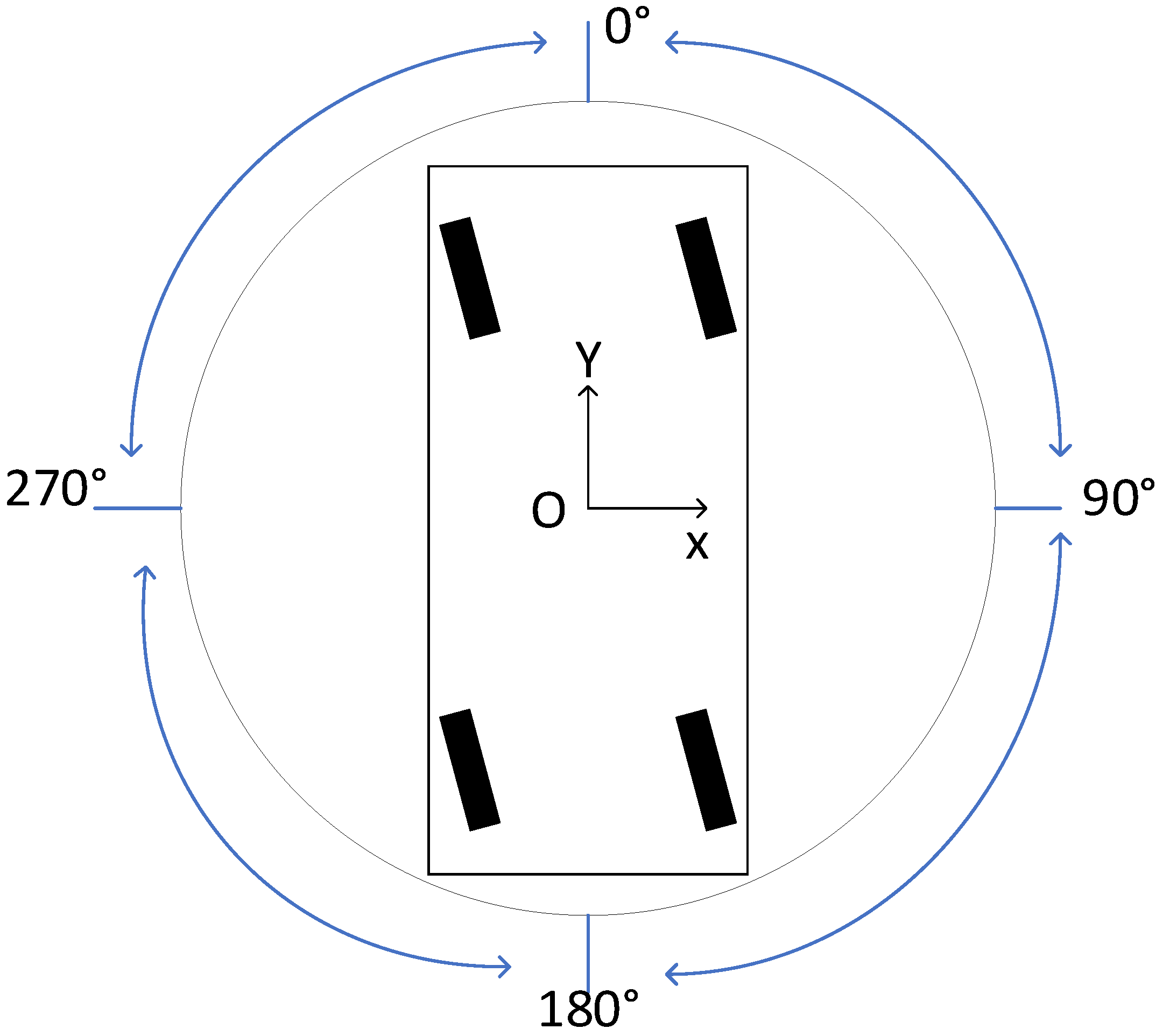
- Steering angle limitation:
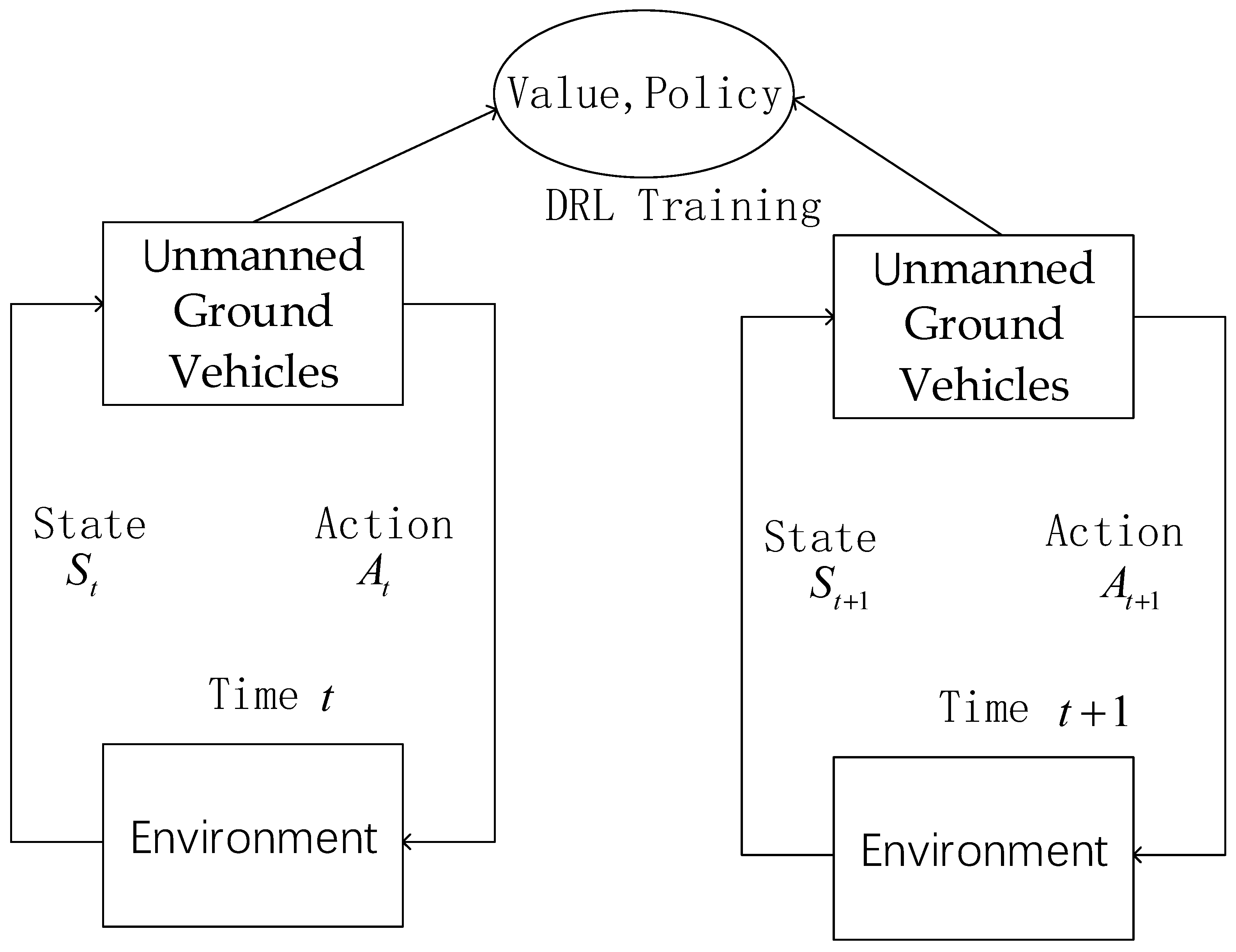
2.2. Unmanned Ground Vehicle Path Planning in Reinforcement Learning
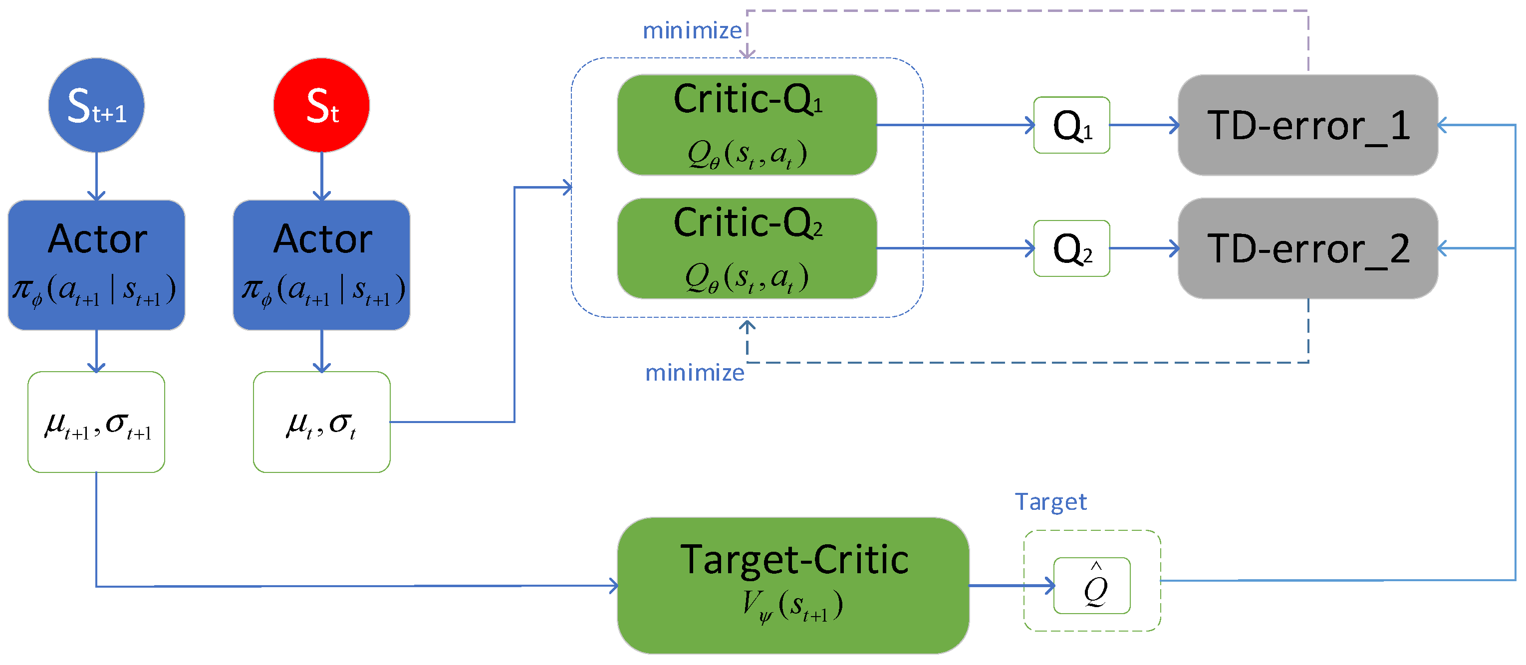
2.3. SAC
| Algorithm 1: The pseudo-code of the general SAC algorithm |
| Initialize parameter vectors , , , for each iteration do for each environment step do end for for each gradient step do end for end for |
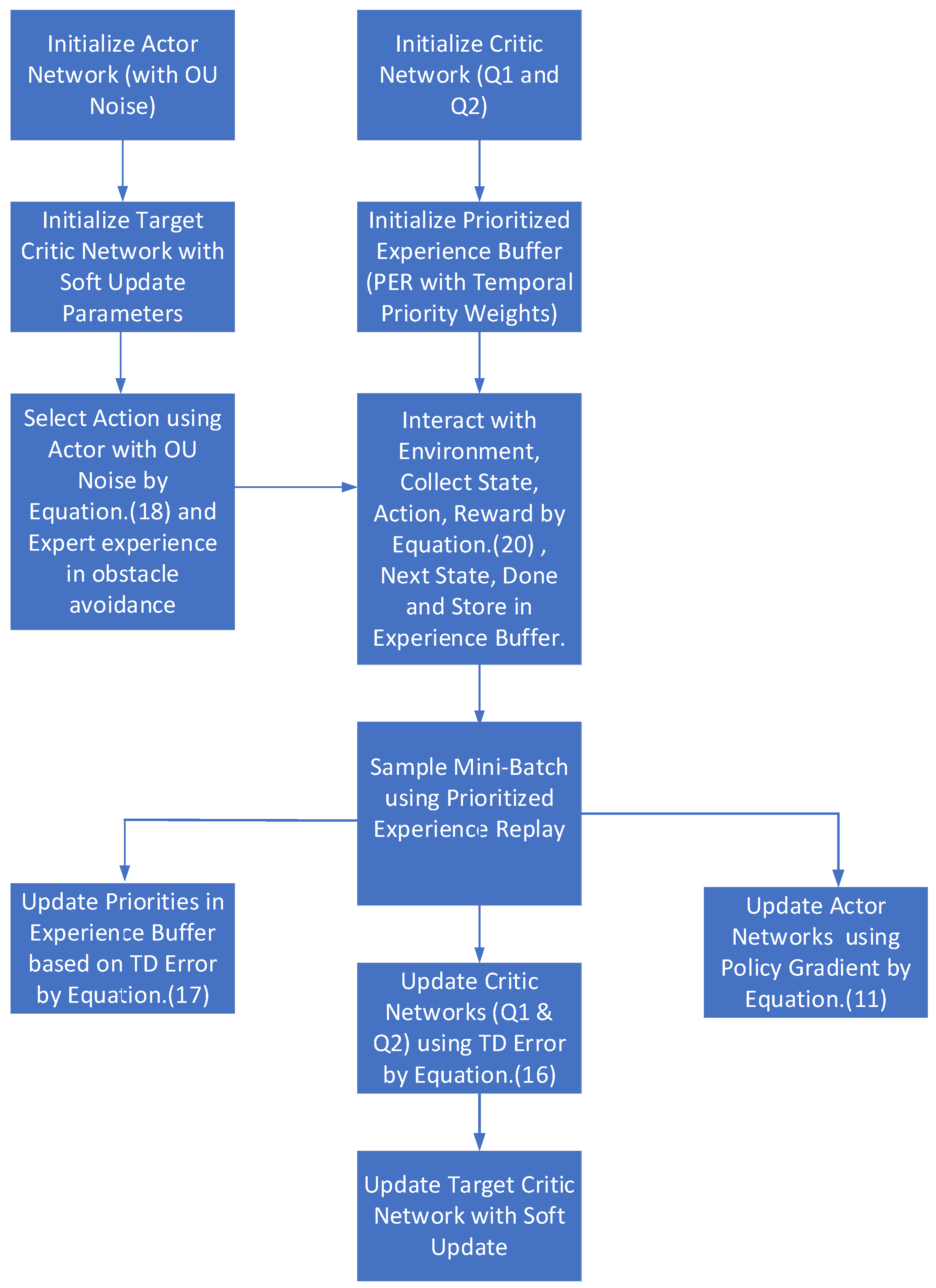
3. Method
| Algorithm 2: The pseudo-code of the general sampling process of the experience replay buffer |
| Step1. Agent interacts with the environment Step2. Store experience in the replay buffer Step3. Sample from replay buffer according to rules Step4. Update strategies and value functions by buffer |
3.1. Double-Factor Prioritized Sampling Experience Replay
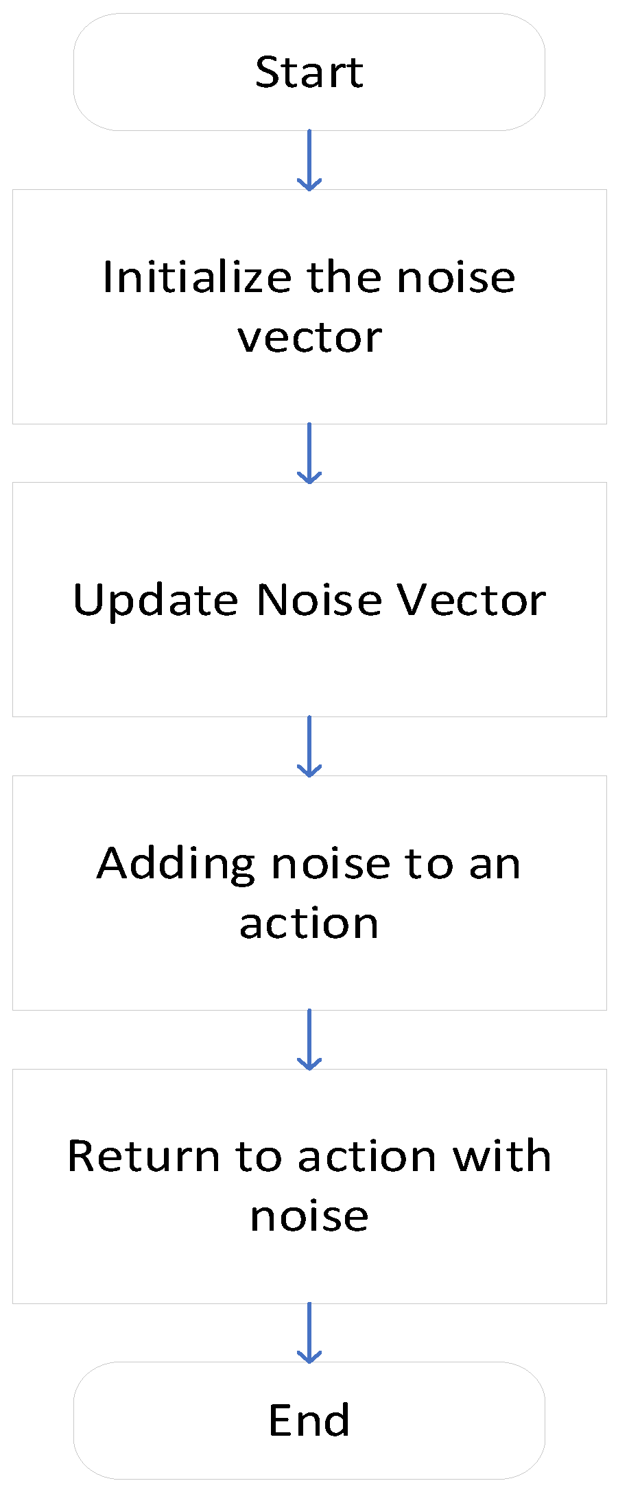
3.2. OU Noise in Select Action
3.3. Expert Experience
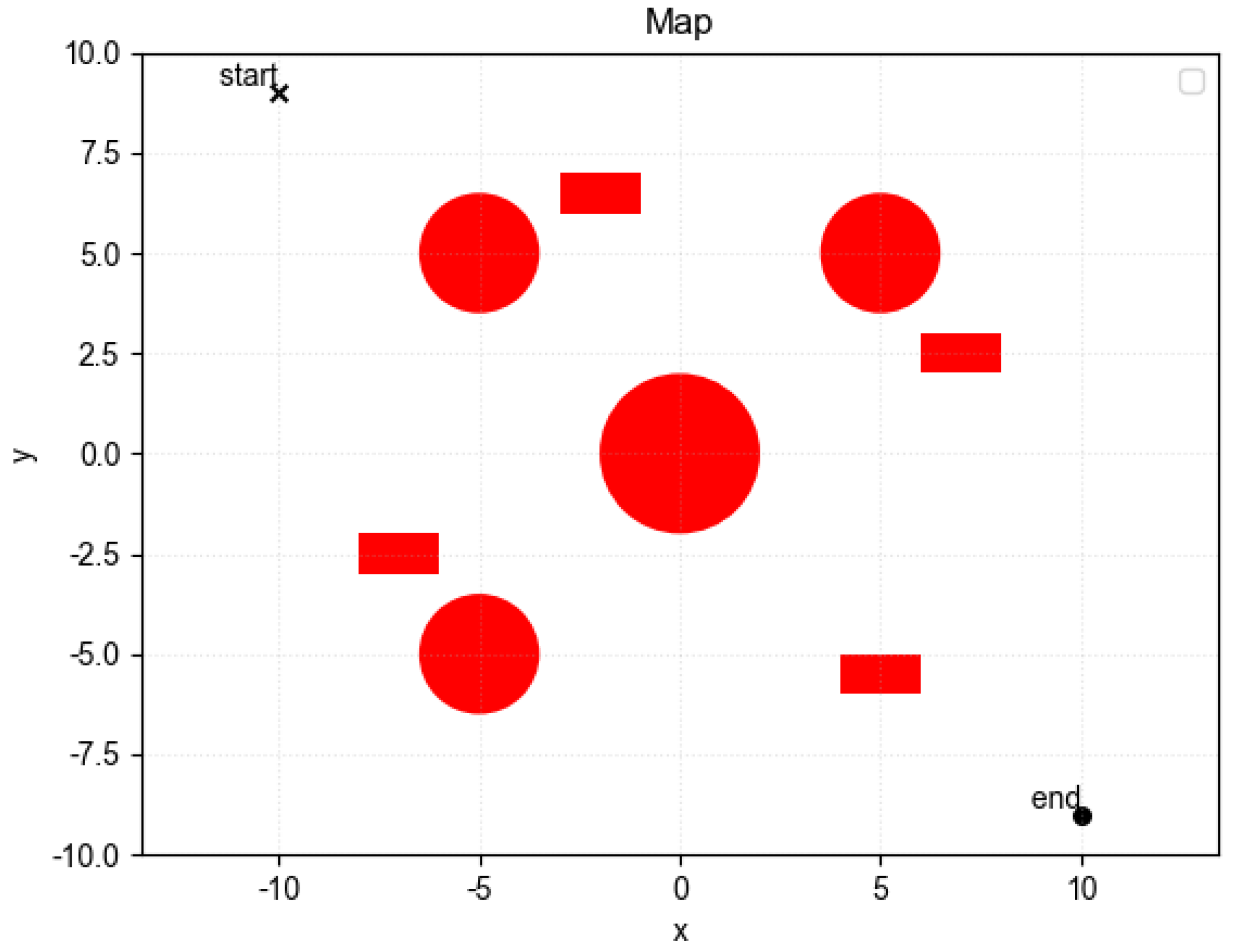
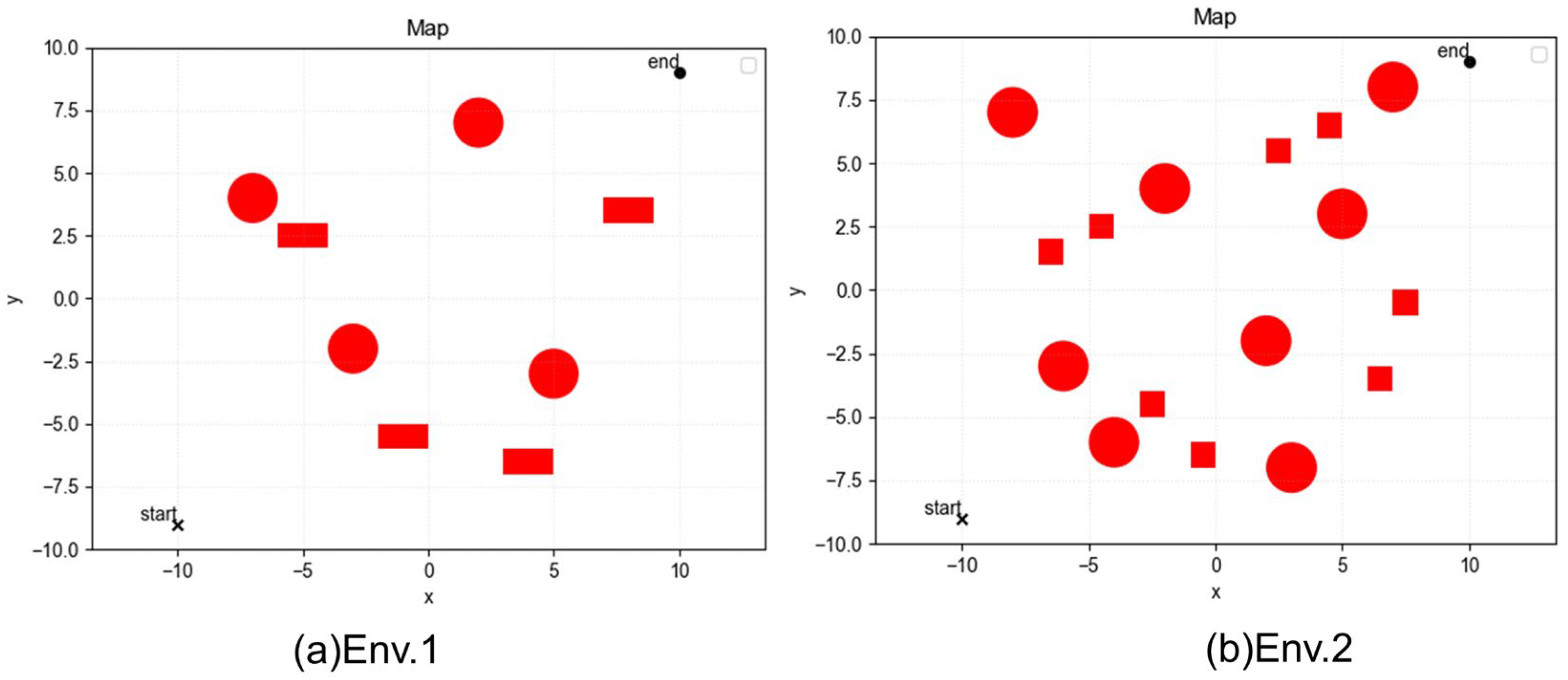
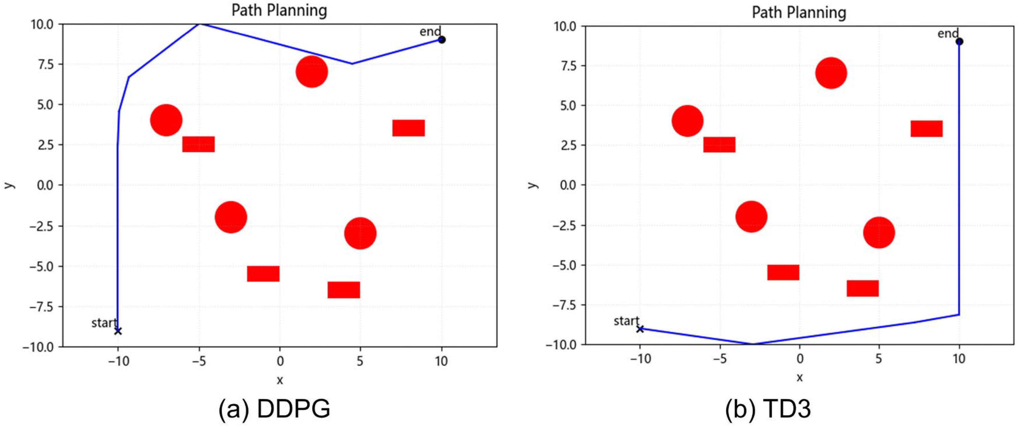
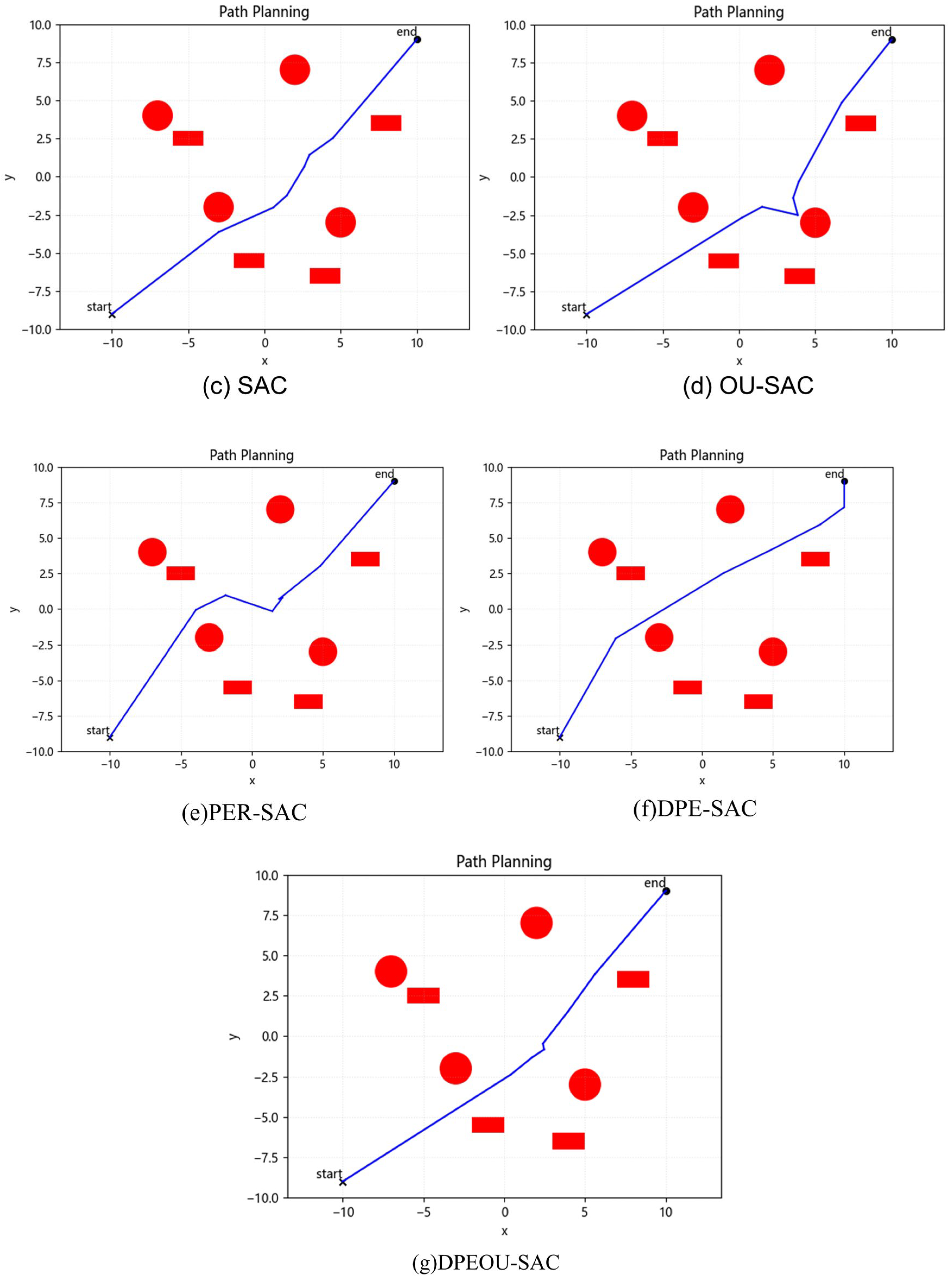
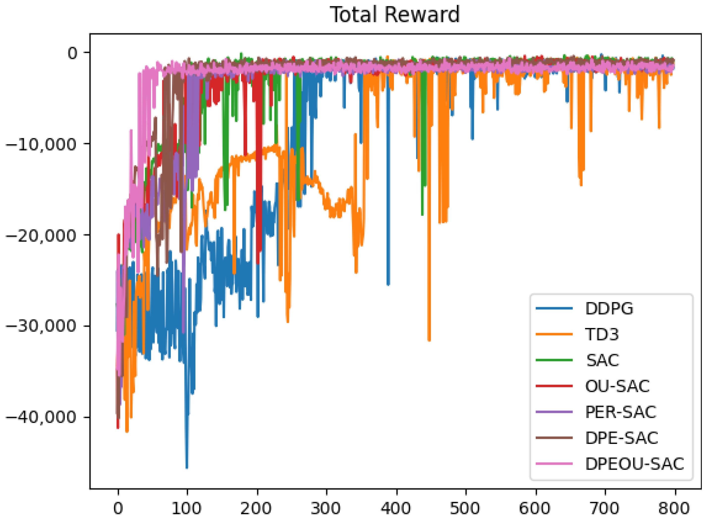
4. Simulations and Analysis
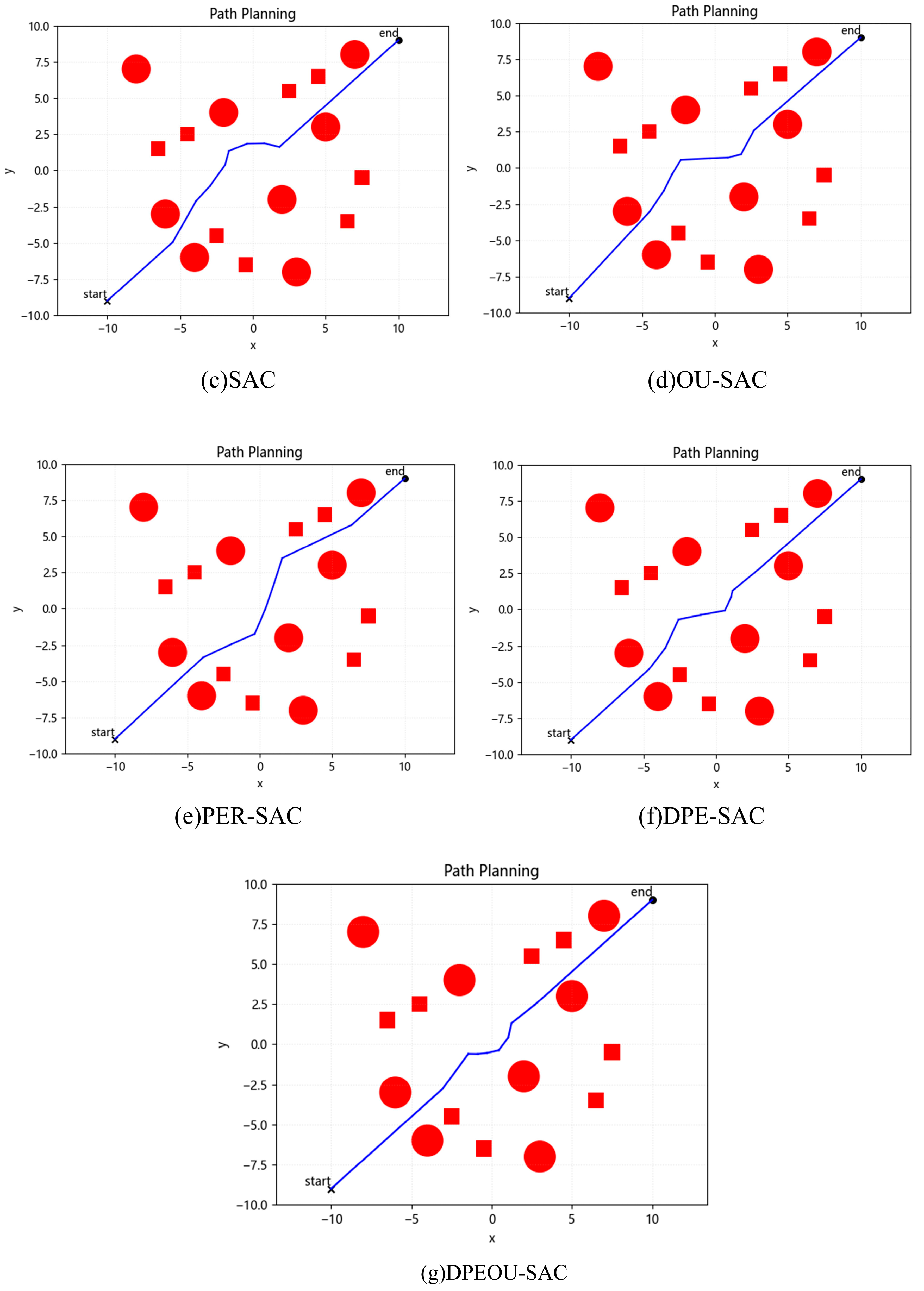
4.1. Static Obstacle Avoidance Simulation Experiments
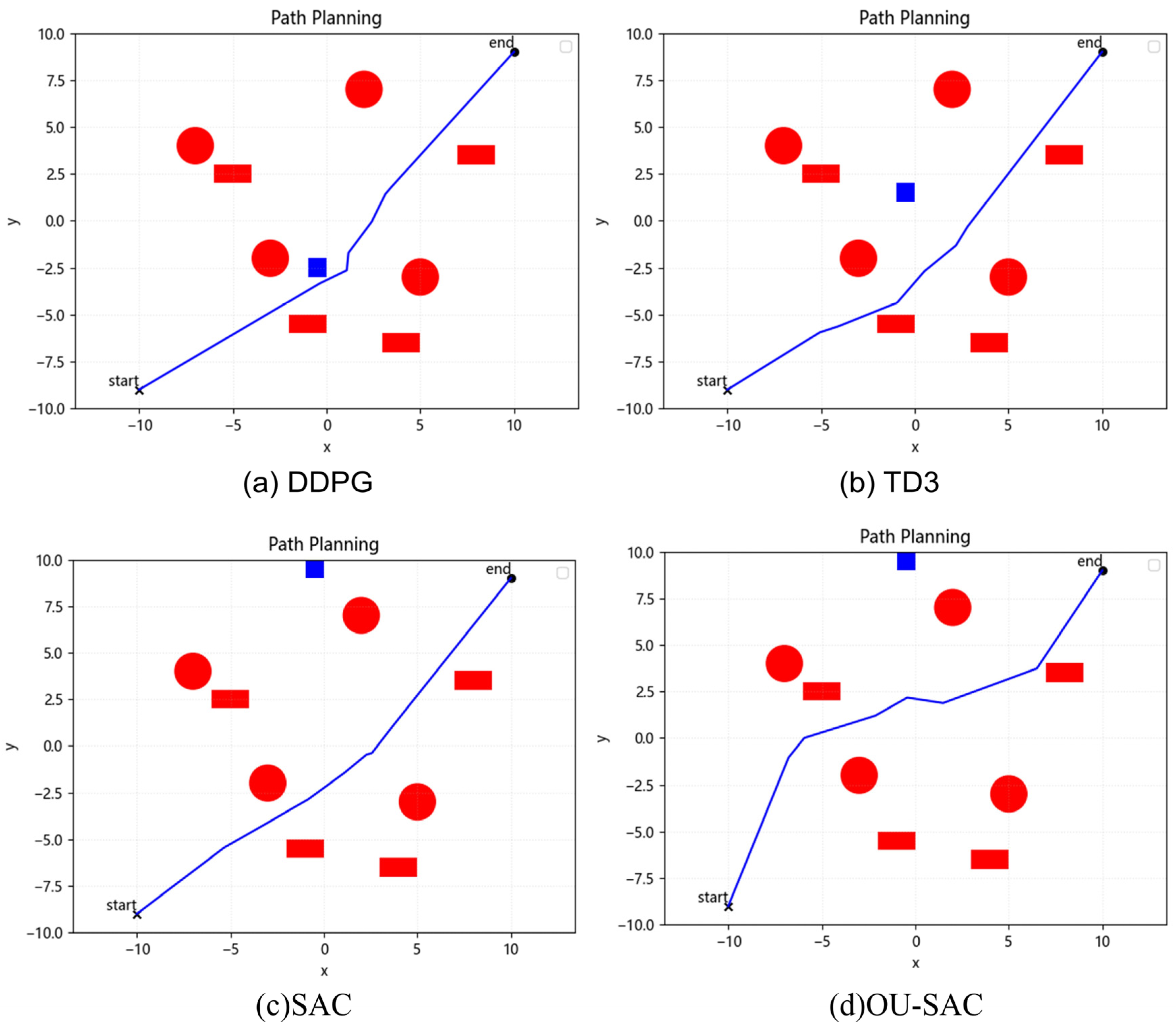
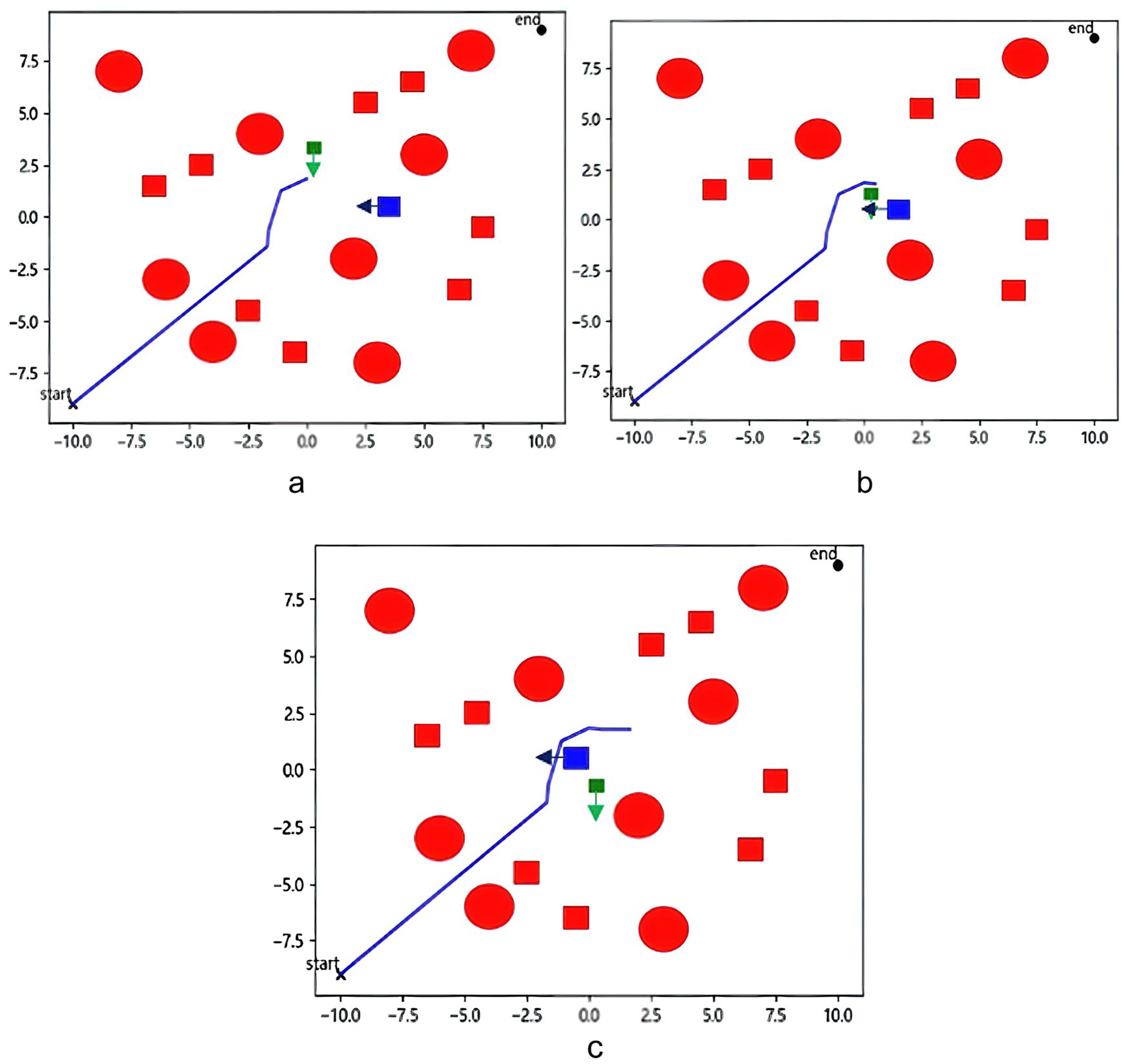
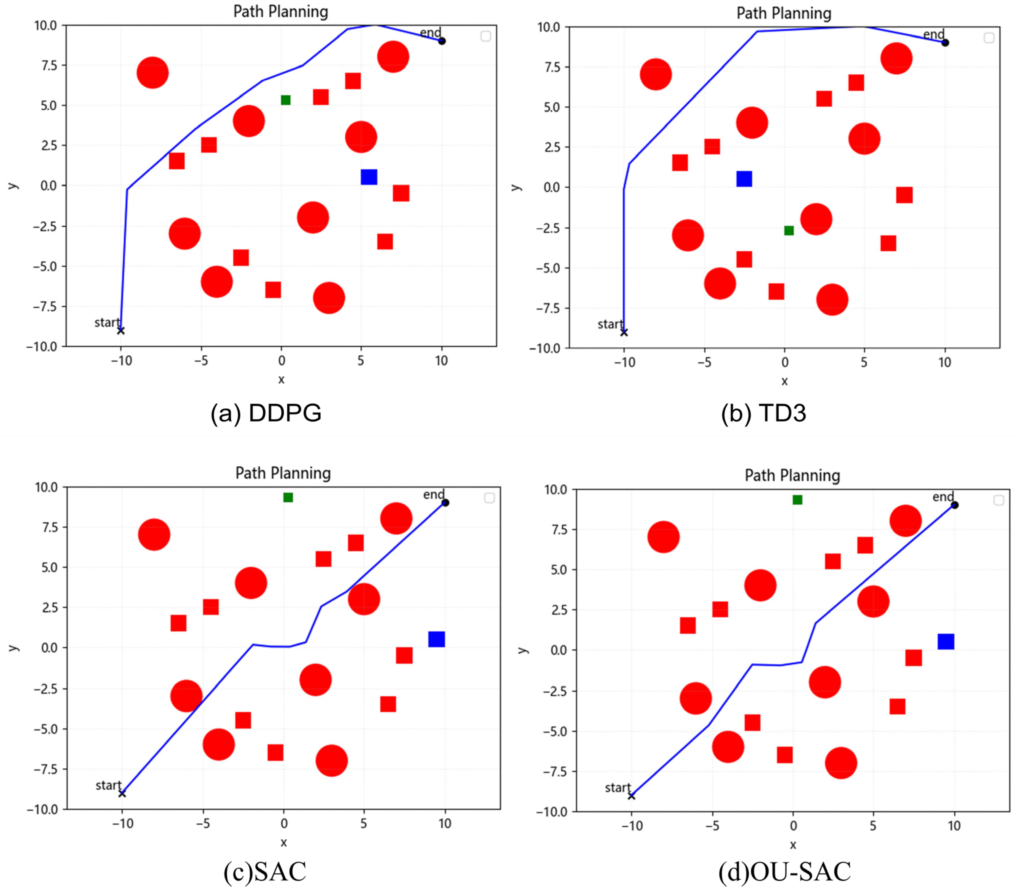
4.2. Dynamic Obstacle Avoidance Experiment
4.3. Impact of Parameter Variations on Algorithm Performance
5. Conclusions and Future Work
Author Contributions
Funding
Data Availability Statement
Conflicts of Interest
References
- Wu, M.; Zhu, S.; Li, C.; Zhu, J.; Chen, Y.; Liu, X.; Liu, R. UAV-Mounted RIS-Aided Mobile Edge Computing System: A DDQN-Based Optimization Approach. Drones 2024, 8, 184. Available online: https://www.mdpi.com/2504-446X/8/5/184 (accessed on 11 May 2024). [CrossRef]
- Alonso-Mora, J.; Baker, S.; Rus, D. Multi-robot formation control and object transport in dynamic environments via constrained optimization. Int. J. Robot. Res. 2017, 36, 1000–1021. [Google Scholar] [CrossRef]
- Su, Z.; Li, M.; Zhang, G.; Yue, F. Modeling and solving the repair crew scheduling for the damaged road networks based on Q-learning. Acta Autom. Sin. 2020, 46, 1467–1478. [Google Scholar]
- Zeng, C.; Yang, C.; Li, Q.; Dai, S. Research progress on human-robot skill transfer. Acta Autom. Sin. 2019, 45, 1813–1828. [Google Scholar]
- Gasparetto, A.; Boscariol, P.; Lanzutti, A.; Vidoni, R. Path planning and trajectory planning algorithms: A general overview. In Motion and Operation Planning of Robotic Systems: Background and Practical Approaches; Springer: Cham, Switzerland, 2015; pp. 3–27. [Google Scholar]
- Raja, P.; Pugazhenthi, S. Optimal path planning of mobile robots: A review. Int. J. Phys. Sci. 2012, 7, 1314–1320. [Google Scholar] [CrossRef]
- Li, Q.; Geng, X. Research on Path Planning Method Based on Improved DQN Algorithm. Comput. Eng. 2023, 1–11. [Google Scholar] [CrossRef]
- Chong, W.; Yi, C.; Shu-Feng, W.; Chaohai, K. Heuristic dynamic path planning algorithm based on SALSTM-DDPG. J. Phys. Conf. Ser. 2023, 2593, 012008. [Google Scholar] [CrossRef]
- Yang, L.; Bi, J.; Yuan, H. Intelligent Path Planning for Mobile Robots Based on SAC Algorithm. J. Syst. Simul. 2023, 35, 1726–1736. [Google Scholar]
- Chen, P.; Pei, J.; Lu, W.; Li, M. A deep reinforcement learning based method for real-time path planning and dynamic obstacle avoidance. Neurocomputing 2022, 497, 64–75. [Google Scholar] [CrossRef]
- Zhang, Y.; Chen, P. Path Planning of a Mobile Robot for a Dynamic Indoor Environment Based on an SAC-LSTM Algorithm. Sensors 2023, 23, 9802. Available online: https://www.mdpi.com/1424-8220/23/24/9802 (accessed on 21 January 2024). [CrossRef]
- Wang, C.; Ross, K. Boosting soft actor-critic: Emphasizing recent experience without forgetting the past. arXiv 2019, arXiv:1906.04009. [Google Scholar]
- Peixoto, M.J.; Azim, A. Using time-correlated noise to encourage exploration and improve autonomous agents performance in Reinforcement Learning. Procedia Comput. Sci. 2021, 191, 85–92. [Google Scholar] [CrossRef]
- Josef, S.; Degani, A. Deep Reinforcement Learning for Safe Local Planning of a Ground Vehicle in Unknown Rough Terrain. IEEE Robot. Autom. Lett. 2020, 5, 6748–6755. [Google Scholar] [CrossRef]
- Liu, Y.; He, Q.; Wang, J.; Chen, T.; Jin, S.; Zhang, C.; Wang, Z. Convolutional Neural Network Based Unmanned Ground Vehicle Control via Deep Reinforcement Learning. In Proceedings of the 2022 4th International Conference on Control and Robotics (ICCR), Guangzhou, China, 2–4 December 2022; pp. 1–6. [Google Scholar] [CrossRef]
- Chen, X.; Qi, Y.; Yin, Y.; Chen, Y.; Liu, L.; Chen, H. A Multi-Stage Deep Reinforcement Learning with Search-Based Optimization for Air–Ground Unmanned System Navigation. Appl. Sci. 2023, 13, 2244. Available online: https://www.mdpi.com/2076-3417/13/4/2244 (accessed on 20 January 2024). [CrossRef]
- Lozano-Pérez, T.; Wesley, M.A. An algorithm for planning collision-free paths among polyhedral obstacles. Commun. ACM 1979, 22, 560–570. [Google Scholar] [CrossRef]
- Gao, P.; Liu, Z.; Wu, Z.; Wang, D. A global path planning algorithm for robots using reinforcement learning. In Proceedings of the 2019 IEEE International Conference on Robotics and Biomimetics (ROBIO), Dali, China, 6–8 December 2019; IEEE: Piscataway, NJ, USA, 2019; pp. 1693–1698. [Google Scholar]
- Xu, X.; Zeng, J.; Zhao, Y.; Lü, X. Research on global path planning algorithm for mobile robots based on improved A. Expert Syst. Appl. 2023, 243, 122922. [Google Scholar] [CrossRef]
- Zong, C.; Han, X.; Zhang, D.; Liu, Y.; Zhao, W.; Sun, M. Research on local path planning based on improved RRT algorithm. Proc. Inst. Mech. Eng. Part D J. Automob. Eng. 2021, 235, 2086–2100. [Google Scholar] [CrossRef]
- Szczepanski, R.; Tarczewski, T.; Erwinski, K. Energy efficient local path planning algorithm based on predictive artificial potential field. IEEE Access 2022, 10, 39729–39742. [Google Scholar] [CrossRef]
- Mnih, V.; Kavukcuoglu, K.; Silver, D.; Rusu, A.A.; Veness, J.; Bellemare, M.G.; Graves, A.; Riedmiller, M.; Fidjeland, A.K.; Ostrovski, G.; et al. Human-level control through deep reinforcement learning. Nature 2015, 518, 529–533. [Google Scholar] [CrossRef]
- Wu, M.; Guo, K.; Li, X.; Lin, Z.; Wu, Y.; Tsiftsis, T.A.; Song, H. Deep Reinforcement Learning-based Energy Efficiency Optimization for RIS-aided Integrated Satellite-Aerial-Terrestrial Relay Networks. IEEE Trans. Commun. 2024, 1. [Google Scholar] [CrossRef]
- Sutton, R.S.; Barto, A.G. Reinforcement Learning: An Introduction; MIT Press: Cambridge, MA, USA, 2018. [Google Scholar]
- Tang, J.; Liang, Y.; Li, K. Dynamic Scene Path Planning of UAVs Based on Deep Reinforcement Learning. Drones 2024, 8, 60. Available online: https://www.mdpi.com/2504-446X/8/2/60 (accessed on 11 May 2024). [CrossRef]
- Haarnoja, T.; Zhou, A.; Abbeel, P.; Levine, S. Soft Actor-Critic: Off-Policy Maximum Entropy Deep Reinforcement Learning with a Stochastic Actor. In Proceedings of the 35th International Conference on Machine Learning, Proceedings of Machine Learning Research, Stockholm, Sweden, 10–15 July 2018; Available online: https://proceedings.mlr.press/v80/haarnoja18b.html (accessed on 12 July 2023).
- Hessel, M.; Modayil, J.; Van Hasselt, H.; Schaul, T.; Ostrovski, G.; Dabney, W.; Horgan, D.; Piot, B.; Azar, M.; Silver, D. Rainbow: Combining improvements in deep reinforcement learning. In Proceedings of the AAAI conference on Artificial Intelligence, New Orleans, LA, USA, 2–7 February 2018; Volume 32. [Google Scholar]
- Christodoulou, P. Soft actor-critic for discrete action settings. arXiv 2019, arXiv:1910.07207. [Google Scholar]
- Banerjee, C.; Chen, Z.; Noman, N. Improved soft actor-critic: Mixing prioritized off-policy samples with on-policy experiences. IEEE Trans. Neural Netw. Learn. Syst. 2022, 35, 3121–3129. [Google Scholar] [CrossRef] [PubMed]
- Jiang, L.; Huang, H.; Ding, Z. Path planning for intelligent robots based on deep Q-learning with experience replay and heuristic knowledge. IEEE/CAA J. Autom. Sin. 2020, 7, 1179–1189. [Google Scholar] [CrossRef]
- Zhang, G.; Wu, Q.; Cui, M.; Zhang, R. Securing UAV communications via joint trajectory and power control. IEEE Trans. Wirel. Commun. 2019, 18, 1376–1389. [Google Scholar] [CrossRef]


| Parameter Name | Value |
|---|---|
| Max_steps | 200 |
| Gamma | 0.99 |
| Alpha | 0.2 |
| Memory_Size | 20,000 |
| Lr_critic | 1 × 10⁻³ |
| Lr_actor | 1 × 10⁻³ |
| Lr_alpha | 1 × 10⁻³ |
| Buffer_alpha_init | 0.6 |
| Buffer_alpha_end | 0.4 |
| Buffer_beta | 0.4 |
| Recentness_weight | 0.1 |
| Batch_size | 128 |
| Algorithm Indicator | DDPG | TD3 | SAC | OU-SAC | PER-SAC | DPE-SAC | DPEOU-SAC |
|---|---|---|---|---|---|---|---|
| collisions converge to 0 | 434 | 672 | 445 | 209 | 112 | 93 | 38 |
| unsmooth converges to 0 | 513 | 672 | 445 | 209 | 118 | 93 | 49 |
| length | 37.46 | 36.72 | 27.47 | 27.91 | 29.14 | 28.34 | 27.31 |
| Algorithm Indicator | OU-SAC | PER-SAC | DPE-SAC | DPEOU-SAC |
|---|---|---|---|---|
| ipc | 53.03% | 74.83% | 79.10% | 88.99% |
| Algorithm Indicator | DDPG | TD3 | SAC | OU-SAC | PER-SAC | DPE-SAC | DPEOU-SAC |
|---|---|---|---|---|---|---|---|
| collisions converge to 0 | 815 | 807 | 534 | 439 | 317 | 300 | 297 |
| unsmooth converges to 0 | 965 | 807 | 534 | 439 | 312 | 301 | 297 |
| length | 35.50 | 35.36 | 27.95 | 28.81 | 27.94 | 27.71 | 27.66 |
| Algorithm Indicator | OU-SAC | PER-SAC | DPE-SAC | DPEOU-SAC |
|---|---|---|---|---|
| ipc | 17.79% | 40.64% | 43.82% | 44.38% |
| Algorithm Indicator | DDPG | TD3 | SAC | OU-SAC | PER-SAC | DPE-SAC | DPEOU-SAC |
|---|---|---|---|---|---|---|---|
| collisions converges to 0 | 369 | 549 | 299 | 254 | 116 | 86 | 59 |
| unsmooth converges to 0 | 368 | 513 | 296 | 253 | 116 | 87 | 59 |
| length | 28.19 | 27.62 | 27.29 | 29.49 | 30.39 | 28.45 | 27.24 |
| Algorithm Indicator | OU-SAC | PER-SAC | DPE-SAC | DPEOU-SAC |
|---|---|---|---|---|
| ipc | 15.05% | 61.20% | 70.90% | 80.27% |
| Algorithm Indicator | DDPG | TD3 | SAC | OU-SAC | PER-SAC | DPE-SAC | DPEOU-SAC |
|---|---|---|---|---|---|---|---|
| collisions converges to 0 | 716 | 719 | 640 | 376 | 432 | 304 | 245 |
| unsmooth converges to 0 | 716 | 426 | 640 | 487 | 432 | 303 | 52 |
| length | 32.16 | 33.57 | 27.98 | 28.04 | 27.92 | 27.89 | 27.64 |
| Algorithm Indicator | OU-SAC | PER-SAC | DPE-SAC | DPEOU-SAC |
|---|---|---|---|---|
| ipc | 23.90% | 32.50% | 52.50% | 61.72% |
| Env | Changed Parament | Fixed Parameter | DPEOU-SAC Convergence Round | DPEOU-SAC Length |
|---|---|---|---|---|
| Env.1 | Gamma1 = 0.97 | Lr = 1 × 10⁻³ | 54 | 28.31 |
| Gamma2 = 0.9 | 75 | 27.64 | ||
| Gamma3 = 0.8 | 122 | 27.94 | ||
| Lr1 = 1 × 10⁻³ | Gamma = 0.95 | 95 | 29.32 | |
| Lr2 = 5 × 10⁻⁴ | 121 | 27.98 | ||
| Lr3 = 1 × 10⁻⁴ | 170 | 27.88 | ||
| Gamma1 Lr1 | None | 84 | 27.66 | |
| Gamma2 Lr2 | 78 | 27.83 | ||
| Gamma3 Lr3 | 157 | 29.73 | ||
| Env.2 | Gamma1 = 0.97 | Lr = 1 × 10⁻³ | 277 | 27.12 |
| Gamma2 = 0.9 | 349 | 28.49 | ||
| Gamma3 = 0.8 | 424 | 28.61 | ||
| Lr1 = 1 × 10⁻³ | Gamma = 0.95 | 442 | 27.84 | |
| Lr2 = 5 × 10⁻⁴ | 348 | 29.64 | ||
| Lr3 = 1 × 10⁻⁴ | 398 | 28.96 | ||
| Gamma1 Lr1 | None | 337 | 27.82 | |
| Gamma2 Lr2 | 412 | 27.29 | ||
| Gamma3 Lr3 | 433 | 27.56 | ||
| Env.3 | Gamma1 = 0.97 | Lr = 1 × 10⁻³ | 83 | 28.53 |
| Gamma2 = 0.9 | 107 | 27.53 | ||
| Gamma3 = 0.8 | 77 | 27.57 | ||
| Lr1 = 1 × 10⁻³ | Gamma = 0.95 | 112 | 27.44 | |
| Lr2 = 5 × 10⁻⁴ | 120 | 27.28 | ||
| Lr3 = 1 × 10⁻⁴ | 144 | 27.06 | ||
| Gamma1 Lr1 | None | 86 | 27.55 | |
| Gamma2 Lr2 | 63 | 28.25 | ||
| Gamma3 Lr3 | 100 | 29.62 | ||
| Env.4 | Gamma1 = 0.97 | Lr = 1 × 10⁻³ | 205 | 28.28 |
| Gamma2 = 0.9 | 228 | 27.31 | ||
| Gamma3 = 0.8 | 255 | 27.35 | ||
| Lr1 = 1 × 10⁻³ | Gamma = 0.95 | 280 | 27.51 | |
| Lr2 = 5 × 10⁻⁴ | 275 | 27.76 | ||
| Lr3 = 1 × 10⁻⁴ | 312 | 27.21 | ||
| Gamma1 Lr1 | None | 235 | 28.22 | |
| Gamma2 Lr2 | 287 | 28.30 | ||
| Gamma3 Lr3 | 310 | 27.53 |
Disclaimer/Publisher’s Note: The statements, opinions and data contained in all publications are solely those of the individual author(s) and contributor(s) and not of MDPI and/or the editor(s). MDPI and/or the editor(s) disclaim responsibility for any injury to people or property resulting from any ideas, methods, instructions or products referred to in the content. |
© 2024 by the authors. Licensee MDPI, Basel, Switzerland. This article is an open access article distributed under the terms and conditions of the Creative Commons Attribution (CC BY) license (https://creativecommons.org/licenses/by/4.0/).
Share and Cite
Liu, L.; Chen, J.; Zhang, Y.; Chen, J.; Liang, J.; He, D. Unmanned Ground Vehicle Path Planning Based on Improved DRL Algorithm. Electronics 2024, 13, 2479. https://doi.org/10.3390/electronics13132479
Liu L, Chen J, Zhang Y, Chen J, Liang J, He D. Unmanned Ground Vehicle Path Planning Based on Improved DRL Algorithm. Electronics. 2024; 13(13):2479. https://doi.org/10.3390/electronics13132479
Chicago/Turabian StyleLiu, Lisang, Jionghui Chen, Youyuan Zhang, Jiayu Chen, Jingrun Liang, and Dongwei He. 2024. "Unmanned Ground Vehicle Path Planning Based on Improved DRL Algorithm" Electronics 13, no. 13: 2479. https://doi.org/10.3390/electronics13132479
APA StyleLiu, L., Chen, J., Zhang, Y., Chen, J., Liang, J., & He, D. (2024). Unmanned Ground Vehicle Path Planning Based on Improved DRL Algorithm. Electronics, 13(13), 2479. https://doi.org/10.3390/electronics13132479