Advanced 3D Navigation System for AGV in Complex Smart Factory Environments

Abstract

The advancement of Industry 4.0 has significantly propelled the widespread application of automated guided vehicle (AGV) systems within smart factories. As the structural diversity and complexity of smart factories escalate, the conventional two-dimensional plan-based navigation systems with fixed routes have become inadequate. Addressing this challenge, we devised a novel mobile robot navigation system encompassing foundational control, map construction positioning, and autonomous navigation functionalities. Initially, employing point cloud matching algorithms facilitated the construction of a three-dimensional point cloud map within indoor environments, subsequently converted into a navigational two-dimensional grid map. Simultaneously, the utilization of a multi-threaded normal distribution transform (NDT) algorithm enabled precise robot localization in three-dimensional settings. Leveraging grid maps and the robot’s inherent localization data, the A* algorithm was utilized for global path planning. Moreover, building upon the global path, the timed elastic band (TEB) algorithm was employed to establish a kinematic model, crucial for local obstacle avoidance planning. This research substantiated its findings through simulated experiments and real vehicle deployments: Mobile robots scanned environmental data via laser radar and constructing point clouds and grid maps. This facilitated centimeter-level localization and successful circumvention of static obstacles, while simultaneously charting optimal paths to bypass dynamic hindrances. The devised navigation system demonstrated commendable autonomous navigation capabilities. Experimental evidence showcased satisfactory accuracy in practical applications, with positioning errors of 3.6 cm along the x-axis, 3.3 cm along the y-axis, and 4.3° in orientation. This innovation stands to substantially alleviate the low navigation precision and sluggishness encountered by AGV vehicles within intricate smart factory environments, promising a favorable prospect for practical applications.

1. Introduction

Industry 4.0 originated in Germany. The concept refers to the use of the Internet of Things and information systems to digitize and automate supply, manufacturing, and sales information in production, aiming to achieve personalized, fast, and efficient product supply [1,2,3]. In the smart factory system that complies with Industry 4.0 standards [4], traditional manual transportation faces numerous limitations related to low efficiency and safety hazards. To alleviate these issues, there has been a widespread emphasis on the crucial role of mobile robots in society [5,6]. Smart factories have started utilizing automated guided vehicle (AGV) systems that provide point-to-point autonomous transportation services through QR code guidance, 2D LiDAR, or visual navigation methods [7,8,9]. AGVs are capable of autonomous navigation based on requirements, offering flexibility and adaptability. They can reduce the need for human resources while ensuring quality and efficiency, thus improving transportation efficiency.

1.1. Related Work

The autonomous navigation of mobile robots entails directing entities toward predetermined destinations using real-time observations in a three-dimensional environment. Its core elements include localization, mapping, path planning, and mobility [10]. Present research predominantly centers on distinct navigation methodologies: trajectory navigation employing QR codes and landmarks as guides, GPS navigation depending on GPS positioning, inertial navigation utilizing inertial navigation sensors, and visual navigation and laser navigation predominantly leveraging cameras and LiDAR as sensors [11].

Indoor navigation commonly relies on ground-level QR codes or environmental landmarks for guiding trajectories, notably in compact smart factory settings. However, this method is substantially influenced by the layout of the surrounding environment, creating stability challenges when external conditions undergo changes [12]. Within GPS navigation, Winterhalter [13] introduced a positioning methodology utilizing the Global Navigation Satellite System (GNSS), merging GNSS maps and signals to facilitate independent robot navigation. Tu [14] employed dual RTK-GPS receivers for location and directional feedback. Yet, these approaches are exclusively effective outdoors or in areas with robust signal strength. In indoor settings or areas with limited signal reception, robots encounter difficulty in accurately interpreting signals, hindering autonomous navigation. Inertial navigation methods leverage the Inertial Measurement Unit (IMU) for relative robot positioning, relying on internal accelerometers, gyroscopes, and magnetometers to capture posture data, allowing operation without constraints from environmental factors or usage scenarios, demonstrating superior adaptability. However, IMU sensors are susceptible to noise, resulting in accumulated errors during extended use, thereby compromising navigation precision [15].

The simultaneous localization and mapping (SLAM) method is a prevalent choice for localization and mapping, leveraging the environmental map and the robot’s present position, considering aspects of its physical control and mobility [16]. SLAM is divided into two main categories based on sensors: visual SLAM and laser SLAM [17,18,19]. In the realm of visual SLAM, Campos and colleagues [20] introduced a groundbreaking visual inertial SLAM system in 2021, tightly integrating IMU with a camera. This pioneering system utilized monocular, stereo, and RGB-D cameras within visual SLAM, significantly improving operational accuracy by two–ten times compared to prior methods, both indoors and outdoors. Qin Tong et al. [21] presented a visual inertial system utilizing a monocular camera and a cost-effective IMU, employing a tightly coupled nonlinear optimization approach that amalgamates pre-integrated measurements and feature observations, achieving high-precision visual-inertial odometry. Additionally, this system underwent four degrees of freedom pose graph optimization to enhance global consistency and remains compatible with mobile devices like smartphones. Visual SLAM technology, primarily employing cameras as the main sensors, delivers rich environmental information at a lower cost, becoming a focal point in current SLAM research. Researchers proposed a positioning and navigation method for service robots based on visual SLAM and visual sensors [22]. The system underwent validation using the Pepper robot platform, encountering limitations in large-scale navigation due to the platform’s short-range laser and RGB depth cameras. Validation encompassed two diverse environments: a medium-sized laboratory and a hall. However, challenges persist in visual SLAM technology, including camera sensitivity to lighting, heightened environmental prerequisites, and limited adaptability. Furthermore, due to its feature-rich nature, visual SLAM demands substantial computational resources, remaining in the experimental phase without commercialization.

Laser SLAM technology, widely used in navigation, employs laser radar sensors to model the environment, generating detailed 2D grid maps crucial for subsequent localization and path planning. Google’s Cartographer [23], an open-source SLAM algorithm, plays a significant role in constructing efficient 2D maps, providing robust support for positioning and planning in robotics and autonomous vehicles. Other commonly utilized laser SLAM mapping algorithms include Gmapping and Karto SLAM. However, these 2D SLAM algorithms adept at indoor mapping encounter challenges in feature loss within long corridors and texture-sparse environments, thereby impacting map accuracy. Additionally, their 2D nature limits the representation of height information in real scenes, resulting in a scale information deficit. In response to these limitations, 3D laser SLAM technology emerged, employing multi-line laser radar to replicate real working environments accurately, giving rise to various 3D SLAM techniques. Lin et al. [24] proposed an enhanced LiDAR Odometry and Mapping (LOAM) algorithm, customized for narrow field-of-view and irregular laser radar. Their refinements in point selection, iterative pose estimation, and parallelization facilitated real-time odometry and map generation, surpassing the original algorithm. Shang et al. [25] introduced a tightly coupled LiDAR-inertial odometry framework. Leveraging IMU pre-integration for motion estimation, they optimized LiDAR odometry and corrected point cloud skewness. Their approach involved estimating IMU biases, integrating keyframe and sliding window strategies, enhancing accuracy, and improving real-time system performance. Xu et al. [26] devised an efficient and robust laser-inertial odometry framework. Employing a tightly coupled iterative extended Kalman filter, they merged laser radar feature points with IMU data, enabling precise navigation in high-speed and complex environments. Their novel formula for computing the Kalman gain notably boosted real-time capabilities. Remarkably, over 1200 valid feature points were fused in a single scan, completing all iterations of the tterated extended Kalman filter (IEKF) step within 25 milliseconds.

Yu et al. [27] devised the ACO-A* dual-layer optimization algorithm, amalgamating ant colony optimization (ACO) with A* search to tackle path planning complexities in obstacle-rich settings. This approach employs ACO for sequential progression determination towards the target, followed by fine-tuning the A* heuristic function for optimal path derivation. Modeling environments at various granularities enabled them to attain optimal paths in intricate settings. Rosas [28] introduced the membrane evolution artificial potential field (MEMEAPF) method, a fusion of membrane computing, genetic, and artificial potential field algorithms, aimed at optimizing path planning by considering minimal path length, safety, and smoothness. Surpassing APF-based strategies, this method harnessed parallel computing techniques to expedite computations, heightening its efficacy and real-time adaptability in dynamic scenarios. Addressing discrepancies in traditional local path planning frameworks, Jian et al. [29] identified potential lateral overshoot and maneuverability reduction during lane changes, impacting ADS modules and vehicle functionality. To combat these challenges, they proposed a multi-model-based framework. Comprising path planning, speed control, and scheduling layers, this structure dynamically generates paths, adjusts speed according to the path, and adapts scheduling based on environmental and vehicle conditions. Consequently, the multi-model approach rectifies limitations inherent in conventional planning methods.

1.2. Contributions and Structure

An extensive review of autonomous navigation systems for AGVs in smart factory settings reveals shortcomings in GPS, trajectory, and inertial navigation. These methods demonstrate limitations in terms of adapting to diverse scenarios and scales. While visual navigation offers intricate feature data, it demands substantial computational resources and encounters constraints in intricate pathways, varying scales, or environments with significant lighting fluctuations. Laser navigation, primarily reliant on 2D maps, lacks comprehensive information and struggles to maintain navigation precision during sudden robot posture changes.

In response, this paper introduces the Complex Scene Navigation System (CSNS). Its key contributions include: designing an adaptable AGV navigation system tailored for intricate smart factory environments; proposing a rapid 3D mapping and localization technique distinct from conventional 2D SLAM approaches, achieving heightened localization precision via 3D point cloud maps; devising a path fusion algorithm based on real-world scenarios; validating the system’s efficacy through extensive simulation experiments and real-world vehicle deployment, achieving navigation accuracy at the centimeter level.

The paper’s structure unfolds as follows: Section 2 delineates the CSNS system framework, detailing the principles governing 3D point cloud maps, 2D grid maps, 3D point cloud localization, and integrated path planning. Section 3 encompasses both simulation and real vehicle experiments, offering a quantitative analysis of navigation accuracy. Finally, Section 4 consolidates the experimental findings and presents avenues for future research.

2. Complex Scene Navigation System CSNS

2.1. System Framework

This paper outlines the design of the navigation system—as depicted in Figure 1—primarily divided into motion model design, mapping, localization, and integrated path planning. Initially, considering the usage scenarios, a motion model equipped with multi-line LiDAR is constructed. The mapping module processes environmental data sensed by sensors to create both a 3D point cloud map and a 2D grid map. The localization module performs real-time alignment between the surrounding point cloud and the 3D point cloud map, enabling real-time self-localization. By transforming the multi-line LiDAR into a single-line LiDAR and removing ground point clouds, the integrated path planning module utilizes information from the single-line LiDAR to execute global optimal path searching and local obstacle avoidance functions on the grid map.

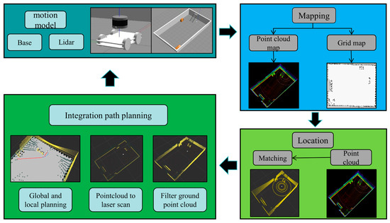
Figure 1. System framework.

2.2. Mapping and Positioning

Currently, the prevalent framework in SLAM is the graph optimization-based model [30,31,32]. The essence of employing graph optimization in SLAM lies in constructing maps and achieving real-time localization by leveraging available observational data. Figure 2 delineates the structure of the graph-based optimization SLAM framework. Under the theoretical framework of graph optimization, the SLAM problem conducts environmental modeling and pose estimation through point cloud segmentation, feature extraction, laser odometry, and map construction. Leveraging an existing point cloud map, the localization problem is transformed into a maximum likelihood estimation-based optimization problem by partitioning the map into several grids conforming to Gaussian distributions. Specifically, the upper right section of Figure 2 illustrates the graph optimization SLAM problem. In this context, the robot’s pose node is symbolized as $\mu =\{{\mu }_1,{\mu }_2,\dots \dots {\mu }_n\}$, while environmental landmarks are represented as $K=\{K_1,K_2,\dots \dots K_n\}$. At time $j$, the robot detects landmark $K_j$ using laser radar at pose ${\mu }_j$, a relationship expressible through observation equations:

$$K_j=F\left({\mu }_j\right).$$

(1)

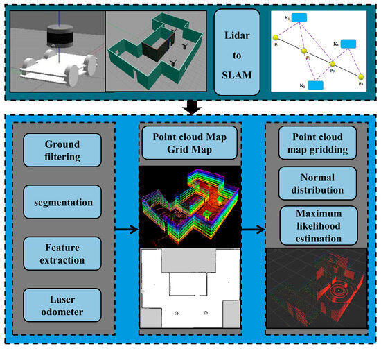
Figure 2. SLAM framework.

Due to sensor noise effects, actual observational data and theoretical observational data do not align [32,33]. Equation (1) does not equate due to the presence of error $e_j=K_j-F\left({\mu }_j\right)$. To minimize this error, the following is introduced:

$$\underset{\mu }{min}{F}_j({\mu }_j)=\parallel e_j\parallel .$$

(2)

At this stage, utilizing Equation (2) as the objective function and treating the pose $\mu$ as the optimization variable enables the computation of refined pose estimations. This process facilitates the inference of the robot’s movement trajectory. Employing the aforementioned equations transforms the SLAM problem into a least squares optimization problem.

2.2.1. Establishment of Point Cloud Map and Grid Map

Point cloud map construction mainly involves point cloud segmentation, feature point extraction, laser odometry, and point cloud map building [33]. Initially, preprocessing is applied to the original point cloud, conducting segmentation. For the point cloud set $P_t=\{p_1,p_2,...,p_n\}$ generated by the LiDAR at time $t$, this study projects the point cloud set into a range image, facilitating subsequent discrete processing. Given the scenario where the robot traverses an incomplete horizontal surface, it is necessary to extract ground points and exclude their application in subsequent segmentation. Subsequently, an image segmentation-based method is applied to the range image, dividing the point cloud set $P_t$ into multiple clusters, assigning unique labels to points within the same cluster. Following this process, the range image not only retains label information about ground points and segmented points but also includes row–column indices of points within the image and their depth values concerning the LiDAR. This segmentation of the point cloud effectively enhances the efficiency of subsequent feature extraction and matching.

After segmenting the original point cloud, each cluster of points is categorized into edge feature points and surface feature points based on curvature [34]. In curvature Formula (3), $r_i$ represents the depth value of the $i\_th$ point in the range image. Here, $S$ denotes the set of points centered on point $i$, including five points to the left and right, while $r_j$ signifies depth values in set $S$ that are not equal to $r_i$.

$$c=\frac{1}{\left|S\right|\cdot \parallel r_i\parallel }\parallel {\sum }_{j\in S,j\ne i}(r_j-r_i)\parallel .$$

(3)

The curvature value, represented by $c$, is calculated using Formula (3) and compared to the predefined threshold $c_{th}$. If it surpasses $c_{th}$, it is categorized as an edge feature; otherwise, it falls into the category of a surface feature. To ensure an evenly distributed set of feature points, the range image is divided into six equal sections, extracting an equal number of edge and surface feature points from each segment.

After applying curvature calculation to segment the point cloud into distinct features, the laser odometry computes the pose transformation between successive frames through a point-to-edge and point-to-surface inter-frame matching approach [34]. To improve alignment speed and precision, given the earlier feature point segmentation, it is crucial to consider the current frame’s categorization within the point cloud. Feature points associated with the current frame’s surface elements are identified as ground points. Meanwhile, for the corner points within the current frame, a search is conducted within clusters bearing the same label. This paper employs a Levenberg–Marquardt (L–M) method, slightly modified from [34], in the least squares-based pose optimization. This method involves two L–M optimization stages: initially refining surface feature points to derive their pose details, followed by utilizing the pose constraints from the prior step to further optimize corner points and obtain the remaining pose information. By considering the feature points’ categories while distinguishing point cloud features and conducting inter-frame matching, this strategy significantly improves the efficiency and precision of laser odometry.

The point cloud map module retains previous feature point sets, and links these with the sensor pose. It centers around the current frame’s point cloud, extracting a feature point set within a 100 m range to establish a point cloud graph. Through matching and optimizing the current frame’s point cloud with the 100 m range point cloud, it generates a local point cloud map. Ultimately, the merging of all local point cloud maps results in the creation of the global point cloud map.

The constructed point cloud map is a sparse point cloud map used solely for localization. To facilitate this, it is necessary to convert the 3D point cloud map into a grid map with real physical dimensions [35]. A grid map refers to the grid representation of a map where each grid’s state is either occupied or free. Each grid is represented by $p(s=1)$ for the occupied state probability and $p(s=0)$ for the free state probability. This paper introduces the grid state using the ratio of free to occupied states, denoted as $Odd(s)$, for each grid.

$$Odd(s)=\frac{p(s=1)}{p(s=0)}.$$

(4)

Upon acquiring laser radar observations $z~\left\{\mathrm{0,1}\right\}$, the grid’s state initiates updates influenced by the observation values $z$.

$$Odd(s\mid z)=\frac{p(s=1\mid z)}{p(s=0\mid z)}.$$

(5)

The probability of the grid occupancy status can be expressed using Bayes’ theorem as follows:

$$p(s=1\mid z)=\frac{p(z\mid s=1)p(s=1)}{p\left(z\right)}$$

(6)

$$p(s=0\mid z)=\frac{p(z\mid s=0)p(s=0)}{p\left(z\right)}.$$

(7)

Put Formulas (6) and (7) into $Odd(s\mid z)$:

$$Odd(s\mid z)=\frac{p(z\mid s=1)}{p(z\mid s=0)}\ast \frac{p(s=1)}{p(s=0)}.$$

(8)

Can be written as:

$$Odd(s\mid z)=\frac{p(z\mid s=1)}{p(z\mid s=0)}\ast Odd(s).$$

(9)

Take the logarithm at both ends of Formula (9):

$$logOdd\left(s∣z\right)=log\frac{p\left(z∣s=1\right)}{p\left(z∣s=0\right)}+logOdd\left(s\right).$$

(10)

At this point, there are only values containing measurement items $log\frac{p(z\mid s=1)}{p(z\mid s=0)}$, so the occupancy grid has only two states: occupied and free. Use $S^{+}$ to represent $logOdd\left(s∣z\right),$ the grid state after measurement, and $S^{-}$ to represent $logOdd\left(s\right),$ the grid state before measurement. Combined with the above formula, the grid state in the occupied grid map can be expressed as:

$$S^{+}=S^{-}+log\frac{p(z\mid s=1)}{p(z\mid s=0)}.$$

(11)

In the initial state of occupying the grid map, the probability of grid free and grid occupancy is 0.5. When the LiDAR scans the surrounding environment and generates observation data, the final grid map is obtained by continuously updating Formula (11).

2.2.2. Positioning in Complex Environments

During the robot’s operation, positioning within the map relies on aligning the present point cloud with the 3D point cloud map. However, discrepancies may arise between the current LiDAR-scanned point cloud and the reference point cloud map. These variations might arise from LiDAR inaccuracies or minor environmental changes. To rectify this, this study converts the 3D point cloud into a multivariate normal distribution. Through the optimization and adjustment of transformation parameters, the optimal alignment between the two laser point clouds is achieved [36].

Firstly, the preconstructed point cloud map is processed by gridification, calculating the probability density function based on the points within each grid. Let ${\overrightarrow{y}}_{k=1,\dots ,m}$ represent the scanned points within a grid. In a three-dimensional environment, the probability density function of this grid can be expressed as:

$$f(\overrightarrow{x})=\frac{1}{(2\pi {)}^{\frac{3}{2}}\sqrt{\left|\Sigma \right|}}{e}^{-\frac{(\overrightarrow{x}-\overrightarrow{\mu }{)}^{T\Sigma -1}(\overrightarrow{x}-\overrightarrow{\mu })}{2}},$$

(12)

where the mean and covariance are expressed as:

$$\overrightarrow{\mu }=\frac{1}{m}{\sum }_{k=1}^m{\overrightarrow{y}}_k$$

(13)

$$\mathsf{\Sigma }=\frac{1}{m}{\sum }_{k=1}^m({\overrightarrow{y}}_k-\overrightarrow{\mu }){({\overrightarrow{y}}_k-\overrightarrow{\mu })}^T.$$

(14)

Using a normal distribution to represent segmented point clouds aids in transforming the initially discrete point clouds into a continuously differentiable form, facilitating derivative operations during subsequent optimizations. During point cloud matching, the goal is to identify the pose of the current scan by comparing it with the 3D point cloud map, maximizing the likelihood of the current points aligning with the reference point cloud map. Therefore, it is necessary to optimize the pose changes (rotation, translation) of the current scanned point cloud. Let $\overrightarrow{p}$ represent the pose transformation, and the current scanned point cloud be denoted as $x=\{{\overrightarrow{x}}_1,\dots ,{\overrightarrow{x}}_n\}$. Define the spatial transformation function $T=\left(\overrightarrow{p},{\overrightarrow{x}}_k\right),$ to denote using the pose transformation $\overrightarrow{p}$ to move the current scanned point ${\overrightarrow{x}}_k$. By continuously adjusting the pose, the aim is to find the optimal spatial transformation function that maximizes the probability. This transforms the alignment problem into a maximum likelihood estimation problem:

$$\theta ={\prod }_{k=1}^{n}f\left(T\right(\overrightarrow{p},{\overrightarrow{x}}_k\left)\right).$$

(15)

To solve the maximum likelihood problem, the logarithm of both ends of the equation can be converted into a least squares problem, and then Newton’s method can be applied to adjust the transformation parameters $\overrightarrow{p}$ to obtain the optimal solution.

2.3. Path Planning Fusion Algorithm

After establishing the mapping and localization modules, the robot needs to autonomously plan paths within the environment. The framework for the path planning system is depicted in Figure 3. As this paper employs autonomous planning in a 2D grid map, it necessitates the conversion of 3D information into 2D data. Before initiating the path planning process, ground point cloud exclusion algorithms are applied to eliminate ground-related data points. Subsequently, the 16-beam LiDAR is compressed into a single-line LiDAR. This enables obstacle detection and path planning within the 2D environment using the single-line LiDAR.

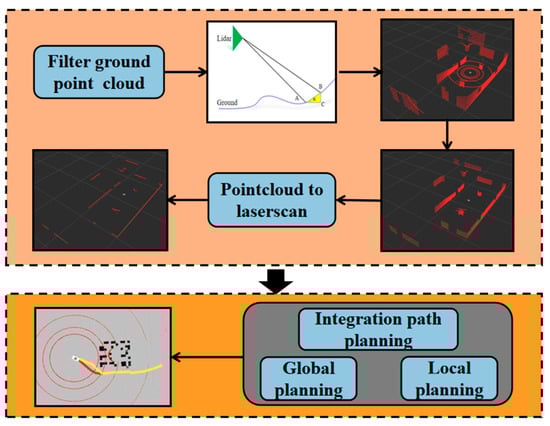
Figure 3. Fusion path planning framework.

2.3.1. Perceptual Data Preprocessing

Although the excessive point cloud generated during the operation of the LiDAR system enriches information, it also adds computational burden to the navigation system [37,38,39]. Therefore, it is imperative to process the point cloud information without compromising accuracy. As illustrated in Figure 3 for ground point cloud filtering, the angle $\alpha$ between points $A$ and $B$ generated by the LiDAR is assessed. If $\alpha$ is less than a predefined threshold—set here as 10 degrees—it is identified as a ground point cloud. Points with $\alpha$ less than 10 degrees are filtered out as ground points. To achieve two-dimensional plane-integrated path planning, the multi-line laser needs conversion into a single-line laser, thereby processing the original point cloud into a ground-free single-line laser.

2.3.2. Fusion Path Planning

The path planning of robotic navigation systems occurs within 2D or 3D environments [40]. Therefore, by establishing a refined grid map, the environment is discretized. Setting the start and goal points within this map, global path planning is achieved by a cost function and depth-first search algorithm to find the shortest path. Initially, starting from the initial point as the center, expanding nodes are determined in the cardinal directions—up, down, left, and right. The optimal expanding node is chosen through a cost function $F=G+H$. Here, $G$ represents the Euclidean distance from the starting point to the expanding node, and $H$ signifies the Euclidean distance from each expanding node to the goal point $E$, considering obstacle-free paths. The node with the minimum $F$ value, calculated through this cost function, is selected as the expanding node.

Subsequently, an open set and a closed set are established. The open set stores the expanding nodes, excluding those deemed as obstacles or belonging to the closed set. The closed set stores the starting point, obstacle nodes, and previously chosen points. If an expanding node belongs to the closed set, it is skipped. Iterating through the open set, the expanding node with the minimum $F$ value is continuously sought until the set contains the goal point. Eventually, the path comprised of all optimal expanding nodes represents the global shortest path.

During robot navigation, encounters with obstacles are inevitable. These obstacles might abruptly appear within the grid map, such as pedestrians, irregularly placed debris, or fallen goods. Hence, it becomes necessary to incorporate local obstacle avoidance design based on the pre-planned global path. The TEB (timed elastic band) [41] algorithm conceptualizes the global path as an ‘elastic band’ and formulates constraints within the algorithm as ‘external forces.’ These forces have the capability to modify local trajectories along the global path, thereby achieving obstacle avoidance effects.

To regulate local variations of the global path based on global path planning, an establishment of constraints is imperative. Initially, within the global path planning, $N$ points are inserted, encompassing the robot’s $x$, $y$ coordinates, and pose information, including its orientation. Uniform motion time is defined between these points. By leveraging the motion time and pose information within each point, the distance between two points can be computed. Differential and second-order differentials of the distance and time provide velocity and acceleration, thus yielding the kinematic information of the mobile robot’s movement.

Subsequently, a graph optimization model is constructed wherein all pose points, time intervals, and obstacles are depicted as nodes, while constraints are represented as edges. Employing graph optimization methods, these discrete poses are organized, ensuring adherence to the robot’s dynamics, forming trajectories that are shortest in time and distance while maintaining a safe distance from obstacles.

3. Experiment and Analysis

3.1. Experimental Setup

To bolster the reliability of the navigation system, the designed system underwent experimentation within the robot operating system (ROS). The hardware setup included a 16-line LiDAR, an i7-11 CPU, and no GPU for enhanced computation. To thoroughly validate the reliability and applicability of the navigation system, the study conducted both simulation-based experiments and real-vehicle trials, accompanied by a quantitative analysis of navigation accuracy.

3.2. Simulation Experiment Verification

3.2.1. Map Building and Localization Performance Analysis

This study was designed to validate the navigation system under a complex simulated environment, as depicted in Figure 4a,b, alongside the point cloud maps of scenes within the CSNS model, demonstrated in Figure 5a,b. The illustrated point cloud maps effectively showcase both the overall map structure and local details. However, due to relatively sparse data acquisition intervals and the laser scanner’s capture of static environments, non-overlapping laser scans occur in the same coordinate system between adjacent poses when the robot’s position remains unchanged. In practice, pose estimation errors and some drift are observed. Extensive experimental testing revealed minimal drift when the vehicle’s speed is below 5 m/s, meeting the practical application requirements.

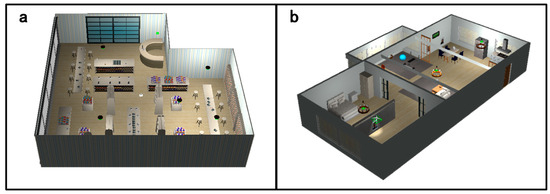
Figure 4. Complex simulated environment. (a,b) depict simulated environments constructed in Gazebo, a simulation software under ROS.

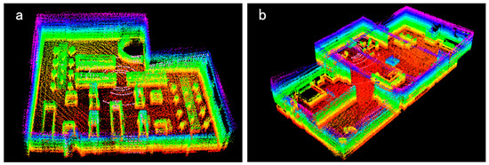
Figure 5. Point cloud map in a simulated environment. (a,b) represent point cloud maps constructed for the simulated environment in Figure 4.

The accuracy of mapping significantly impacts subsequent modules within the navigation system. This study employed Evolution of Visual Odometry and Mapping Datasets (evo) software for evaluating mapping accuracy, depicted in Figure 6a,b. Figure 6a portrays an error analysis comparing the estimated trajectory to the ground truth during mapping. Leveraging ROS’ rviz visualization software in the simulated environment facilitates easy access to the robot’s actual trajectory. Figure 6b vividly showcases the errors encountered in the robot’s mapping process. The figure indicates a maximum error of 0.137 m between estimated and actual trajectories, a minimum of 0.003 m, and an average error of 0.045 m. An analysis of these mapping errors demonstrates the proposed mapping method’s capability to precisely simulate the surrounding environment, aligning with practical application requirements.

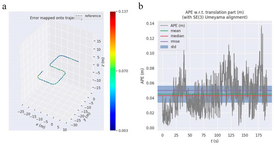
Figure 6. Error analysis in map construction. (a) represents mapping trajectory error, while (b) represents mapping absolute error.

The grid maps constructed by the 2D mapping module are shown in Figure 7a,b. It can be seen that these maps effectively project the 3D point cloud map into a 2D grid map, allowing for a clear representation of obstacle information and map outlines in the images.

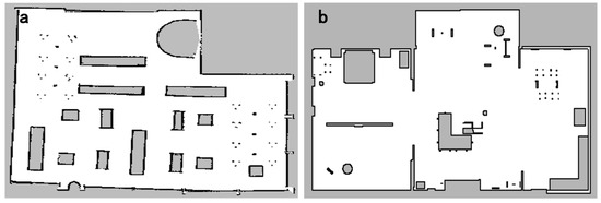
Figure 7. Grid map in a simulated environment. (a,b) demonstrate the process of mapping the point cloud map in Figure 5 into a grid map.

Figure 8a,b depict the localization experiments of the vehicle during autonomous navigation. In the simulated environment, this study conducted the vehicle’s localization with speeds set between 2 m/s and 5 m/s. From Figure 8, it is evident that, during the vehicle’s movement, the current point cloud information precisely matches the original point cloud map.

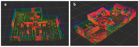
Figure 8. Real-time localization in a simulated environment. (a,b) illustrates the matching process between real-time scanned point cloud data and the point cloud map. The red section represents the real-time point cloud, while the other colors represent the point cloud map.

To enhance the precision of localization quantification, this study employs pose error assessment encompassing both angular and positional discrepancies. The simulation experiments enable the acquisition of the robot’s actual position within the global coordinate system, facilitating an error analysis between the pose information from the localization module and the robot’s global pose data. Figure 9a–c delineate the angular and positional errors (x, y) during the localization process. Figure 9a reveals a maximum angular error of 4.77° with an average deviation of 2.89°. Meanwhile, Figure 9b,c depict maximum errors in the x-direction at 2.91 cm, averaging 1.59 cm, and in the y-direction at 3.19 cm, with an average of 2.08 cm. The localization error encapsulates various factors such as localization algorithms, precision in robot motion control, and hardware configuration. Integrating the aforementioned data, the robot demonstrates centimeter-level localization accuracy within the simulated environment, affirming its ability to accurately ascertain its own position during autonomous navigation.

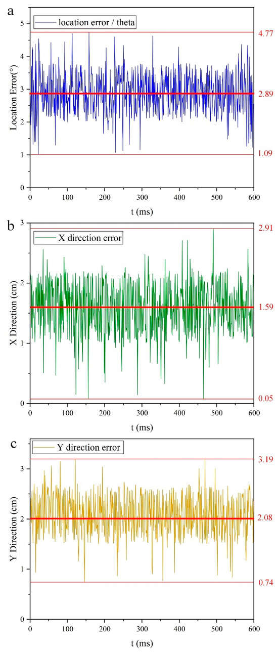
Figure 9. Localization error analysis. (a) represents angular error, (b) represents x-axis error, (c) represents y-axis error.

3.2.2. Path Planning Performance Test

This study evaluates the efficacy of path planning using the rviz tool within the ROS system. Figure 10 and Figure 11 depict the navigation system’s path planning within a simulated environment, where the red lines represent global paths and the yellow lines denote local paths. These visual representations clearly illustrate the navigation system’s capability to intelligently select optimal global paths and dynamically plan local avoidance paths when encountering obstacles. Throughout the testing phase, by iteratively adjusting the positions of target points and obstacles, we observed the navigation system consistently determining optimal routes in the environment, effectively accomplishing obstacle avoidance and halting functionalities.

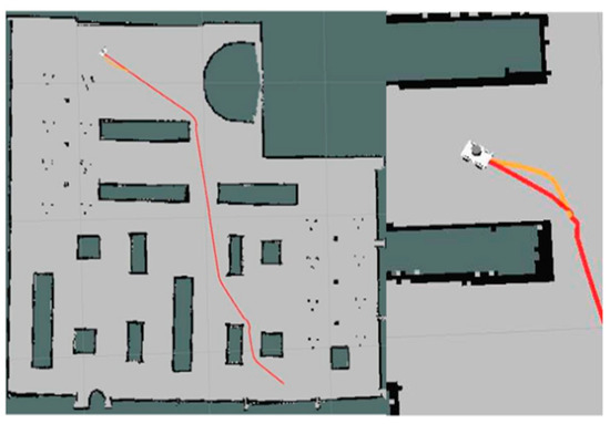
Figure 10. In the navigation experiment of the navigation system in Figure 4a, the red line segment represents the global path, while the yellow line segment represents the local path.

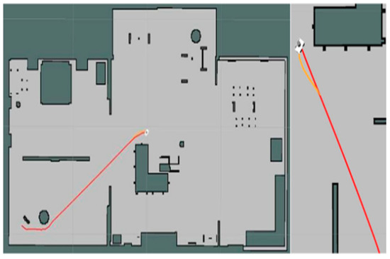
Figure 11. In the navigation experiment of the navigation system in Figure 4b, the red line segment represents the global path, while the yellow line segment represents the local path..

3.3. Real-World Deployment Experiment Verification and Analysis

3.3.1. Map Building and Localization Performance Analysis

In the real-world deployment experiments, the key laboratory of the Zhejiang University of Science and Technology Smart Factory was selected as the experimental environment. The mobile robot was composed of an Ackermann chassis and an RS-LiDAR-16. The control computer for the mobile robot was equipped with an Intel i5-10th generation CPU and operated without GPU acceleration. The experimental environment is depicted in Figure 12a–c. From Figure 12, it is evident that the experimental environment exhibits a complex layout with narrow passageways and significant variations in the height of goods placement. The surrounding environment is not entirely structured, posing a substantial challenge for validating the navigation system.

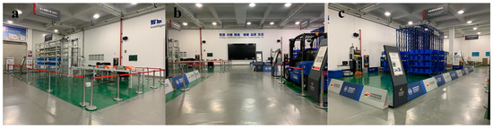
Figure 12. (a–c) are the real environment of the key laboratory of Zhejiang University of Science and Technology.

The mobile robot constructed a 3D point cloud map of the smart factory using the CSNS navigation system, as shown in Figure 13a–c, where Figure 13a corresponds to Figure 12a, and Figure 13c corresponds to Figure 12c. Figure 13b provides a complete aerial view of the smart factory. From the figures, it can be observed that the 3D point cloud map created by the CSNS navigation system accurately reproduces the real environment and effectively captures local details.

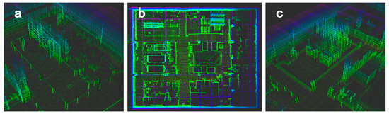
Figure 13. (a–c) correspond to the point cloud maps in Figure 12a, 12b, and 12c, respectively.

The 2D grid map mapped from the 3D point cloud map is shown in Figure 14. By comparing the grid map with the 3D point cloud map, it can be observed that the CSNS navigation system effectively maps the outline of the 3D point cloud map onto the 2D grid map. Additionally, the grid map displays both map contours and obstacle information.

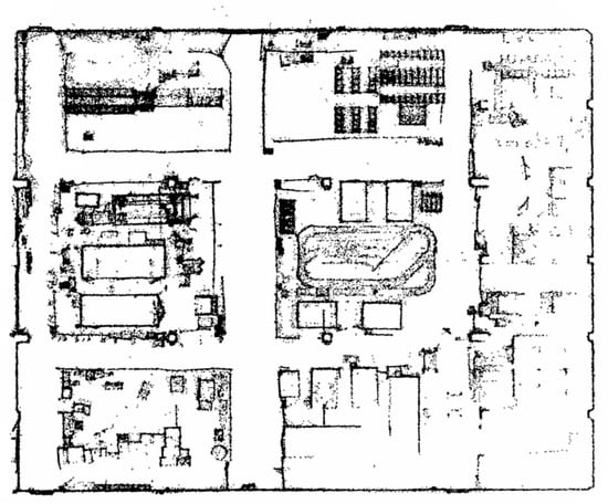
Figure 14. Smart factory grid map.

Similar to the simulation experiments, this study constrained the mobile robot’s velocity within the range of 2 m/s to 5 m/s during the localization experiments. Leveraging the real-time scanning of point cloud data and its alignment with the point cloud map, the mobile robot accurately determined its position in dynamic environments, achieving real-time autonomous localization, as illustrated in Figure 15a–f. Figure 15a corresponds to the real-time autonomous localization of the robot depicted in Figure 15d, similarly, Figure 15b aligns with Figure 15e, and Figure 15c corresponds to Figure 15f. Visually, from the figures, it is apparent that the robot’s pose in the real-world scenario bears minimal deviation from the pose depicted in rviz.

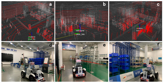
Figure 15. (a) corresponds to the point cloud localization in (d); similarly, (b) corresponds to (e), and (c) corresponds to (f). The red color represents real-time scanned point clouds, while the other colors represent the point cloud map.

3.3.2. Real Vehicle Navigation Test

The A* and Dijkstra algorithms are common global path planning methods based on 2D grid maps. Dijkstra, a well-known breadth-first search algorithm, efficiently determines the shortest path between two points. However, Dijkstra’s algorithm exhibits relatively high time complexity. In contrast, the A* algorithm, enhancing global planning speed by incorporating a heuristic cost function atop Dijkstra’s framework, is presented. Table 1 compares the efficiency of the A* algorithm and Dijkstra’s algorithm in real vehicle experiments considering scenarios with and without obstacles. TEB and DWA are prevalent local path planning algorithms. TEB, accounting for robot kinematic constraints, is particularly adaptable to the Ackermann chassis compared to DWA. Both A* and TEB algorithms are encapsulated within ROS packages, ensuring enhanced compatibility with upper-level mapping and localization modules.

Table 1. Comparison of path planning efficiency.

Algorithm	With Obstacles	Without Obstacles
A*algorithm	2.3 s	1.8 s
Dijkstra algorithm	3.0 s	2.5 s

In practical navigation deployment tests, obtaining the robot’s precise positional information within the actual environment proves exceedingly challenging. Consequently, a lack of actual pose serves as a reference point. To effectively evaluate the accuracy of the navigation system in real-world settings, this study adopted an assessment method akin to that of reference [42]. By establishing identical start and end points, the navigation system underwent ten iterative tests, allowing for a comparison between the robot’s positional information in the real environment and that observed in rviz, showcasing specific errors as depicted in Figure 16a–c.

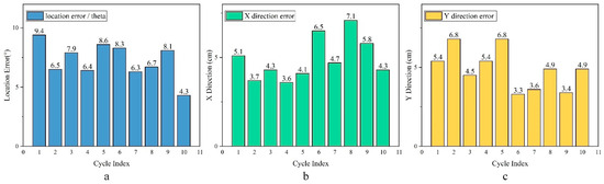
Figure 16. (a) represents angular error, (b) represents x-axis error, and (c) represents y-axis error.

Figure 16a illustrates the angular errors across ten iterative tests within the real vehicle environment, with a maximum angular error of 9.4°, a minimum of 4.3°, and an average of 7.5°. Figure 16b,c depict positional errors, with a maximum error of 7.1 cm along the x-axis and an average error of 5 cm. Along the y-axis, the maximum error reaches 6.8 cm, with an average of 4.9 cm. When comparing these error metrics with simulation data, noticeable elevation in errors during real vehicle experiments is evident. This increase is attributed to sensor noise and the difficulty in acquiring the robot’s true positional information within real-world settings. Nonetheless, the overall errors in the real vehicle environment remain within the centimeter range, meeting practical requirements.

Figure 17a–c illustrate the process of navigation testing, encompassing both global and local path planning. The visuals depict the generation of seamless global paths between start and end points, ensuring an optimized distance from obstacles while maintaining utmost safety. Additionally, the system exhibits the capability to proactively devise local avoidance paths when encountering sudden obstacles during vehicle movement.

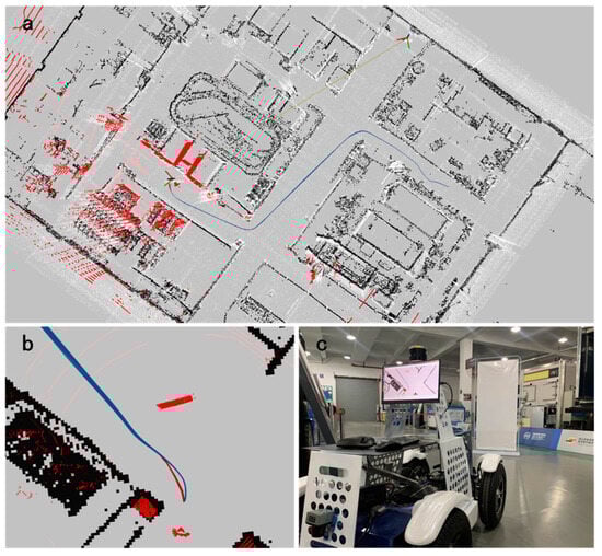
Figure 17. (a) depicts path planning under the grid map, in (b), the dark blue line represents the global path, the red line represents the local path, and (c) represents the robot’s obstacle avoidance process.

4. Conclusions

In response to the inherent challenges of low accuracy and slow speed within complex smart factory environments using traditional two-dimensional navigation systems, this paper presents a novel design for a complex scene navigation system. The system comprises four key components: motion model design, map construction, localization, and fused path planning. The motion model integrates an Ackermann steering chassis and multi-line laser radar. The map construction module utilizes multi-line laser radar to capture surrounding point cloud data, subsequently processed through point cloud segmentation, feature point extraction, laser odometry, and map construction, thereby generating a point cloud map. Additionally, this map is transformed into a grid map suitable for fused path planning. The localization module standardizes the point cloud map and optimizes pose as a variable, reducing real-time registration errors between the live point cloud and the map. The fused path planning module streamlines computation complexity by eliminating ground points from the point cloud, converting multi-line laser data to single-line laser data, establishing a cost function and leveraging this function alongside a depth-first traversal algorithm to achieve the globally optimal path at the lowest cost. Essentially, global path constraints are introduced to govern local path variations. Finally, a graph optimization method generates an optimal trajectory comprising discrete poses while adhering to dynamic constraints. Experimental validation demonstrates that the navigation system achieves centimeter-level precision in simulated environments. The average error on the x-axis is 1.59 cm, on the y-axis is 2.08 cm, and the average orientation error is 2.89 degrees. In real vehicle experiments, despite a slight decrease in navigation accuracy due to experimental constraints and sensor noise, the system still ensures stable and accurate autonomous robot navigation. This highlights the system’s excellent performance in controlled environments, acknowledging potential influences of various factors during actual deployment. Future enhancements may prioritize reducing sensor noise, optimizing system parameters, and enhancing adaptability in real-world application scenarios to further augment system performance and stability. Overall, the CSNS navigation system has proven to be highly suitable for autonomous navigation in complex environments such as smart factories and industrial parks.

References

- Castelo-Branco, I.; Amaro-Henriques, M.; Cruz-Jesus, F.; Oliveira, T. Assessing the Industry 4.0 European divide through the country/industry dichotomy. Comput. Ind. Eng. 2023, 176, 108925. [Google Scholar] [CrossRef]
- Ortt, R.; Stolwijk, C.; Punter, M. Implementing Industry 4.0: Assessing the current state. J. Manuf. Technol. Manag. 2020, 31, 825–836. [Google Scholar] [CrossRef]
- Asif, M. Are QM models aligned with Industry 4.0? A perspective on current practices. J. Clean. Prod. 2020, 258, 120820. [Google Scholar] [CrossRef]
- Kalsoom, T.; Ramzan, N.; Ahmed, S.; Ur-Rehman, M. Advances in sensor technologies in the era of smart factory and industry 4.0. Sensors 2020, 20, 6783. [Google Scholar] [CrossRef] [PubMed]
- Bartneck, C.; Forlizzi, J. A design-centred framework for social human-robot interaction. In Proceedings of the RO-MAN 2004 13th IEEE International Workshop on Robot and Human Interactive Communication (IEEE Catalog No. 04TH8759), Kurashiki, Japan, 22 September 2004. [Google Scholar]
- Kirby, R.; Forlizzi, J.; Simmons, R. Affective social robots. Robot. Auton. Syst. 2010, 58, 322–332. [Google Scholar] [CrossRef]
- dos Reis, W.P.N.; Morandin Junior, O. Sensors applied to automated guided vehicle position control: A systematic literature review. Int. J. Adv. Manuf. Technol. 2021, 113, 21–34. [Google Scholar] [CrossRef]
- Zhang, J.; Yang, X.; Wang, W.; Guan, J.; Ding, L.; Lee, V.C. Automated guided vehicles and autonomous mobile robots for recognition and tracking in civil engineering. Autom. Constr. 2023, 146, 104699. [Google Scholar] [CrossRef]
- Sahoo, S.; Lo, C.-Y. Smart manufacturing powered by recent technological advancements: A review. J. Manuf. Syst. 2022, 64, 236–250. [Google Scholar] [CrossRef]
- Zhou, K.; Zhang, H.; Li, F. TransNav: Spatial sequential transformer network for visual navigation. J. Comput. Des. Eng. 2022, 9, 1866–1878. [Google Scholar] [CrossRef]
- Radočaj, D.; Plaščak, I.; Jurišić, M. Global Navigation Satellite Systems as State-of-the-Art Solutions in Precision Agriculture: A Review of Studies Indexed in the Web of Science. Agriculture 2023, 13, 1417. [Google Scholar] [CrossRef]
- Zhang, Y.; Li, B.; Sun, S.; Liu, Y.; Liang, W.; Xia, X.; Pang, Z. GCMVF-AGV: Globally Consistent Multi-View Visual-Inertial Fusion for AGV Navigation in Digital Workshops. IEEE Trans. Instrum. Meas. 2023, 72, 5030116. [Google Scholar] [CrossRef]
- Winterhalter, W.; Fleckenstein, F.; Dornhege, C.; Burgard, W. Localization for precision navigation in agricultural fields—Beyond crop row following. J. Field Robot. 2021, 38, 429–451. [Google Scholar] [CrossRef]
- Tu, X.; Gai, J.; Tang, L. Robust navigation control of a 4WD/4WS agricultural robotic vehicle. Comput. Electron. Agric. 2019, 164, 104892. [Google Scholar] [CrossRef]
- Li, H.; Ao, L.; Guo, H.; Yan, X. Indoor multi-sensor fusion positioning based on federated filtering. Measurement 2020, 154, 107506. [Google Scholar] [CrossRef]
- Yasuda, Y.D.V.; Martins, L.E.G.; Cappabianco, F.A.M. Autonomous visual navigation for mobile robots: A systematic literature review. ACM Comput. Surv. (CSUR) 2020, 53, 1–34. [Google Scholar] [CrossRef]
- Jia, G.; Li, X.; Zhang, D.; Xu, W.; Lv, H.; Shi, Y.; Cai, M. Visual-SLAM Classical framework and key Techniques: A review. Sensors 2022, 22, 4582. [Google Scholar] [CrossRef]
- Cheng, J.; Zhang, L.; Chen, Q.; Hu, X.; Cai, J. A review of visual SLAM methods for autonomous driving vehicles. Eng. Appl. Artif. Intell. 2022, 114, 104992. [Google Scholar] [CrossRef]
- Zhou, X.; Huang, R. A State-of-the-Art Review on SLAM. In Proceedings of the International Conference on Intelligent Robotics and Applications, Harbin, China, 1–3 August 2022; Springer: Cham, Switzerland, 2022. [Google Scholar]
- Campos, C.; Elvira, R.; Rodriguez, J.J.G.; Montiel, J.M.M.; Tardos, J.D. ORB-SLAM3: An accurate open-source library for visual, visual–inertial, and multimap SLAM. IEEE Trans. Robot. 2021, 37, 1874–1890. [Google Scholar] [CrossRef]
- Qin, T.; Li, P.; Shen, S. VINS-Mono: A robust and versatile monocular visual-inertial state estimator. IEEE Trans. Robot. 2018, 34, 1004–1020. [Google Scholar] [CrossRef]
- Silva, J.R.; Simão, M.; Mendes, N.; Neto, P. Navigation and obstacle avoidance: A case study using Pepper robot. In Proceedings of the IECON 2019—45th Annual Conference of the IEEE Industrial Electronics Society, Lisbon, Portugal, 14–17 October 2019; Volume 1. [Google Scholar]
- Hess, W.; Kohler, D.; Rapp, H.; Andor, D. Real-time loop closure in 2D LIDAR SLAM. In Proceedings of the 2016 IEEE International Conference on Robotics and Automation (ICRA), Stockholm, Sweden, 16–21 May 2016. [Google Scholar]
- Lin, J.; Zhang, F. Loam livox: A fast, robust, high-precision LiDAR odometry and mapping package for LiDARs of small FoV. In Proceedings of the 2020 IEEE International Conference on Robotics and Automation (ICRA), Paris, France, 31 May–31 August 2020; pp. 3126–3131. [Google Scholar]
- Shan, T.; Englot, B.; Meyers, D.; Wang, W.; Ratti, C.; Rus, D. LIO-SAM: Tightly-coupled lidar inertial odometry via smoothing and mapping. In Proceedings of the 2020 IEEE/RSJ International Conference on Intelligent Robots and Systems (IROS), Las Vegas, NV, USA, 24 October 2020–24 January 2021; pp. 5135–5142. [Google Scholar]
- Xu, W.; Zhang, F. FAST-LIO: A fast, robust LiDAR-inertial odometry package by tightly-coupled iterated kalman filter. IEEE Robot. Autom. Lett. 2021, 6, 3317–3324. [Google Scholar] [CrossRef]
- Yu, X.; Chen, W.-N.; Gu, T.; Yuan, H.; Zhang, H.; Zhang, J. ACO-A*: Ant colony optimization plus A* for 3-D traveling in environments with dense obstacles. IEEE Trans. Evol. Comput. 2018, 23, 617–631. [Google Scholar] [CrossRef]
- Orozco-Rosas, U.; Montiel, O.; Sepúlveda, R. Mobile robot path planning using membrane evolutionary artificial potential field. Appl. Soft Comput. 2019, 77, 236–251. [Google Scholar] [CrossRef]
- Jian, Z.; Chen, S.; Zhang, S.; Chen, Y.; Zheng, N. Multi-model-based local path planning methodology for autonomous driving: An integrated framework. IEEE Trans. Intell. Transp. Syst. 2020, 23, 4187–4200. [Google Scholar] [CrossRef]
- Lu, F.; Milios, E. Globally consistent range scan alignment for environment mapping. Auton. Robot. 1997, 4, 333–349. [Google Scholar] [CrossRef]
- Zhu, H.; Kuang, X.; Su, T.; Chen, Z.; Yu, B.; Li, B. Dual-Constraint Registration LiDAR SLAM Based on Grid Maps Enhancement in Off-Road Environment. Remote Sens. 2022, 14, 5705. [Google Scholar] [CrossRef]
- Jang, W.; Kim, T.-W. iSAM2 using CUR matrix decomposition for data compression and analysis. J. Comput. Des. Eng. 2021, 8, 855–870. [Google Scholar] [CrossRef]
- Shan, T.; Englot, B. LeGO-LOAM: Lightweight and ground-optimized lidar odometry and mapping on variable terrain. In Proceedings of the 2018 IEEE/RSJ International Conference on Intelligent Robots and Systems (IROS), Madrid, Spain, 1–5 October 2018. [Google Scholar]
- Zhang, J.; Singh, S. LOAM: Lidar odometry and mapping in real-time. In Proceedings of the Robotics: Science and Systems, Berkeley, CA, USA, 12–16 July 2014; Volume 2. [Google Scholar]
- Hornung, A.; Wurm, K.M.; Bennewitz, M.; Stachniss, C.; Burgard, W. OctoMap: An efficient probabilistic 3D mapping framework based on octrees. Auton. Robot. 2013, 34, 189–206. [Google Scholar] [CrossRef]
- Magnusson, M. The Three-Dimensional Normal-Distributions Transform: An Efficient Representation for Registration, Surface Analysis, and Loop Detection. Ph.D. Thesis, Örebro Universitet, Örebro, Sweden, 2009. [Google Scholar]
- Li, X.; Du, S.; Li, G.; Li, H. Integrate point-cloud segmentation with 3D LiDAR scan-matching for mobile robot localization and mapping. Sensors 2019, 20, 237. [Google Scholar] [CrossRef]
- Zováthi, Ö.; Nagy, B.; Benedek, C. Point cloud registration and change detection in urban environment using an onboard Lidar sensor and MLS reference data. Int. J. Appl. Earth Obs. Geoinf. 2022, 110, 102767. [Google Scholar] [CrossRef]
- Sun, H.; Deng, Q.; Liu, X.; Shu, Y.; Ha, Y. An Energy-Efficient Stream-Based FPGA Implementation of Feature Extraction Algorithm for LiDAR Point Clouds With Effective Local-Search. IEEE Trans. Circuits Syst. I Regul. Pap. 2022, 70, 253–265. [Google Scholar] [CrossRef]
- Yi, X.; Zhu, A.; Li, C.; Yang, S.X. A novel bio-inspired approach with multi-resolution mapping for the path planning of multi-robot system in complex environments. J. Comput. Des. Eng. 2022, 9, 2343–2354. [Google Scholar] [CrossRef]
- Andreasson, H.; Larsson, J.; Lowry, S. A Local Planner for Accurate Positioning for a Multiple Steer-and-Drive Unit Vehicle Using Non-Linear Optimization. Sensors 2022, 22, 2588. [Google Scholar] [CrossRef] [PubMed]
- Ren, J.; Wu, T.; Zhou, X.; Yang, C.; Sun, J.; Li, M.; Jiang, H.; Zhang, A. SLAM, Path Planning Algorithm and Application Research of an Indoor Substation Wheeled Robot Navigation System. Electronics 2022, 11, 1838. [Google Scholar] [CrossRef]
Disclaimer/Publisher’s Note: The statements, opinions and data contained in all publications are solely those of the individual author(s) and contributor(s) and not of MDPI and/or the editor(s). MDPI and/or the editor(s) disclaim responsibility for any injury to people or property resulting from any ideas, methods, instructions or products referred to in the content. |
© 2023 by the authors. Licensee MDPI, Basel, Switzerland. This article is an open access article distributed under the terms and conditions of the Creative Commons Attribution (CC BY) license (https://creativecommons.org/licenses/by/4.0/).