Abstract
Convolutional neural networks (CNNs) have transformed the landscape of image analysis and are widely applied across various fields. With their widespread adoption in fields like medical diagnosis and autonomous driving, CNNs have demonstrated powerful capabilities. Despite their success, existing models face challenges in deploying and operating in resource-constrained environments, limiting their practicality in real-world scenarios. We introduce LMFRNet, a lightweight CNN model. Its innovation resides in a multi-feature block design, effectively reducing both model complexity and computational load. Achieving an exceptional accuracy of 94.6% on the CIFAR-10 dataset, this model showcases remarkable performance while demonstrating parsimonious resource utilization. We further validate the performance of the model on the CIFAR-100, MNIST, and Fashion-MNIST datasets, demonstrating its robustness and generalizability across diverse datasets. Furthermore, we conducted extensive experiments to investigate the influence of critical hyperparameters. These experiments provided valuable insights for effective model training.
1. Introduction
Convolutional neural networks (CNNs) are a type of deep learning neural network. They have revolutionized various fields, including image classification [1], object detection [2], and image segmentation [3]. CNNs leverage convolutional layers to extract features from input images, and fully connected layers to classify images. This architectural design enables CNNs to capture both local and global information in images, facilitating the learning of relationships between image content and semantics. In various domains, CNNs have been widely applied, demonstrating their versatility and effectiveness [4]. These applications encompass diverse areas such as lesion detection [5,6] and diagnostic support within the medical field, autonomous driving [7], and face recognition [8], among others.
Since the introduction of AlexNet [9], CNNs have undergone rapid development. AlexNet demonstrated the potential of large-scale deep convolutional neural networks for image recognition tasks. It employed an eight-layer convolutional network structure and achieved breakthrough performance on the ImageNet dataset. Subsequently, VGGNet [10] simplified network design by stacking small convolutional filters to achieve a balance between depth and efficiency. The Inception [11] module enabled CNNs to learn more complex feature representations by combining filters of different sizes. The ResNet [12] architecture effectively addressed the vanishing gradient problem, enabling the construction of models with over a hundred layers. DenseNet [13] promoted efficient feature reuse by connecting every layer to every other layer.
Deep learning models have achieved significant success in the field of image analysis, demonstrating outstanding accuracy in tackling challenging image recognition tasks. However, improving accuracy often implies increased demands on computational resources.
Real-world tasks often demand optimal accuracy within constrained resources, influenced by factors such as the specific platform requirements and diverse application scenarios [14,15,16,17]. Merely pursuing accuracy might constrain their practical applicability on resource-limited mobile devices. Therefore, designing a model that balances parameter quantity and accuracy is a challenging task.
As a result, some lightweight models have emerged, such as SqueezeNet, ShuffleNet-V2, MobileNetV2, and EfficientNet. SqueezeNet [18] decreases the model size by compressing convolutional filters and employing a small number of 1x1 convolutional kernels. ShuffleNet-V2 [19] reduces computational costs through group convolution and channel shuffling techniques, maintaining strong performance in resource-constrained environments. MobileNetV2 [20] reduces the number of parameters by using Depthwise Separable Convolution, making it suitable for deployment on mobile and embedded devices. EfficientNet [21] adopts compound scaling, balancing model depth, width, and resolution to enhance performance while retaining a relatively compact model size.
In this study, inspired by these classic models, we introduce LMFRNet, a lightweight network designed specifically for image classification tasks. The experimental results demonstrate that the proposed model achieves an exceptional accuracy of 94.6% on the CIFAR-10 dataset, despite having only 0.52 million parameters. It was compared to state-of-the-art (SOTA) models on the CIFAR-10 dataset, and the model achieved superior accuracy under equivalent parameter conditions. Additionally, we substantiate the model’s effectiveness through validation on the CIFAR-100, MNIST, and Fashion-MNIST datasets. Furthermore, the model does not use residual blocks, which also provides an idea for exploring scenarios without such blocks. This underscores the efficiency and feasibility of the model. In addition, we conducted extensive experiments to investigate the influence of critical hyperparameters, providing valuable insights for effective model training.
This study contributes to the following:
- First, we propose a lightweight model that attains an outstanding accuracy of 94.6% on the CIFAR-10 dataset, leveraging a mere 0.52 million parameters. Notably, in equivalent parameter setups, the model surpasses existing SOTA models, showcasing a remarkable balance between performance and parameter efficiency.
- Second, we conducted an extensive array of experiments to carefully adjust various common hyperparameters, including training epochs, optimizer selection, data augmentation strategies, and learning rates. By comparing the performance of different hyperparameter settings, we provide valuable experimental results to help practitioners better understand and apply these critical parameters, facilitating more effective model training.
2. Method
In the section, we deconstruct the fundamental CNN components that constitute the model’s underlying architecture. Building upon these core components, we now delve deeper into the intricate architecture of our proposed model, dissecting its components in detail. Figure 1 visually represents the model, showcasing its six stages, each playing a crucial role in progressively extracting pertinent features from the input image, ultimately yielding the desired classification output.
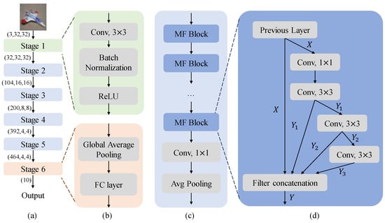
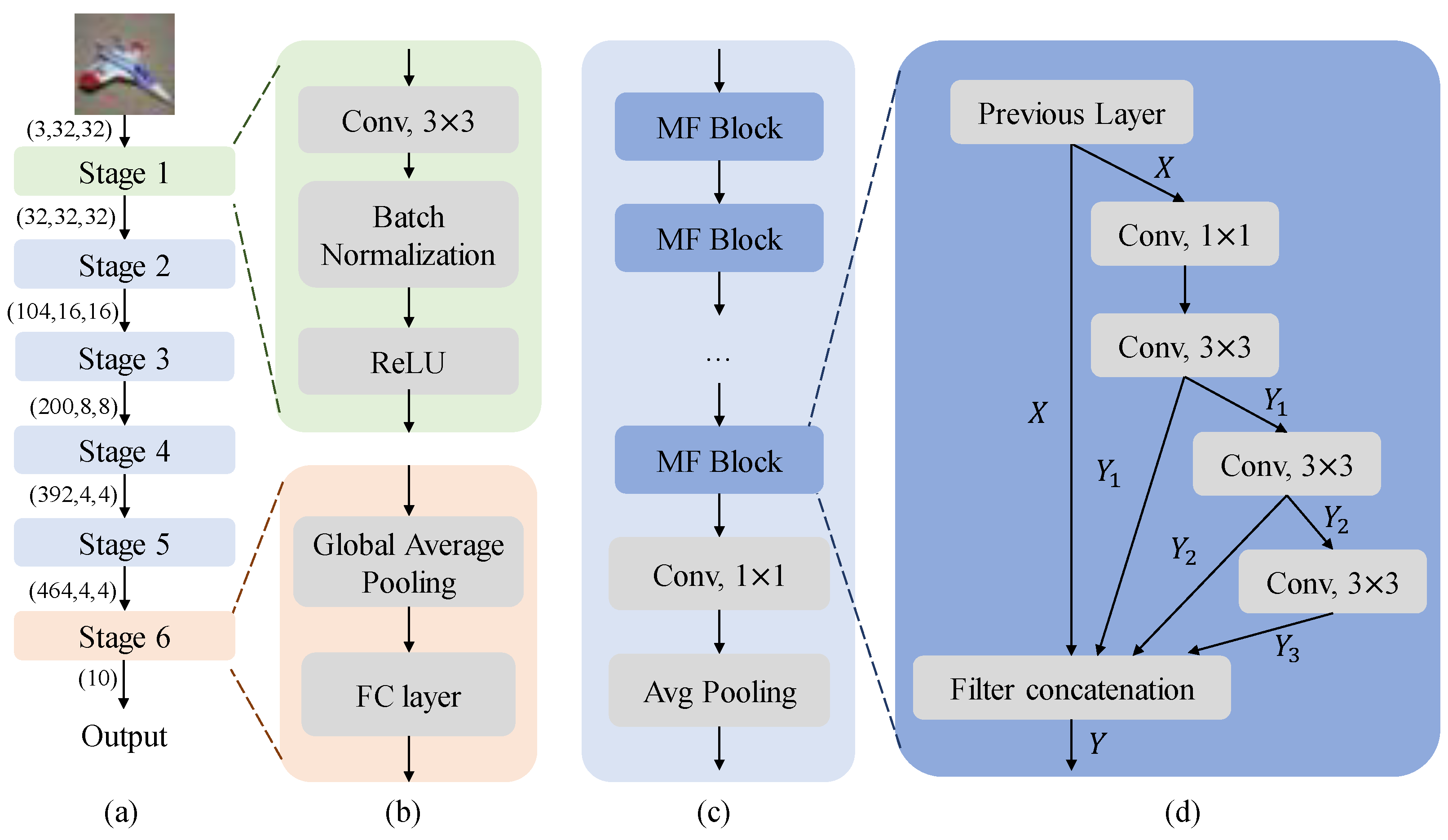
Figure 1.
(a) The architectural overview of the proposed model. (b) The structure of Stage 1 and Stage 6. (c) The overall structure of Stages 2 through 5. (d) The structure of MF block.
2.1. Basic CNN Components
Convolutional layers are the most important elements of CNNs [9,10]. They are responsible for extracting features from the input data. Convolutional layers work by applying a convolution operation to the input data. The convolution operation [22] is defined as follows:
In this equation, represents the element in the output feature map at position , represents the element in the input data at position , and signifies the weight of the convolutional kernel at position . The indices m and n iteratively cover all possible positions within the convolutional kernel, performing the crucial convolution operation across the input data. This fundamental operation plays a pivotal role in extracting meaningful features from the input, which is instrumental for CNNs in various tasks.
Pooling layers are used to reduce the spatial dimensions of the feature maps [9,12]. The purpose of this is to reduce the computational cost of the network and to make the network more robust to noise. Max pooling operates by selecting the maximum value within each region of the feature map, while average pooling computes the average value within these regions. Additionally, global average pooling (GAP) represents a unique pooling operation aimed at condensing the spatial dimensions of a feature map into a single vector [11,12]. This is achieved by computing the average value across each channel in the feature map.
Batch normalization [23] is a technique that is used to improve the stability and generalization ability of CNNs. It is defined as follows:
Here, x represents input data, is the mean of the input data, is the variance of the input data, and are learnable scaling and shifting parameters, and is a small constant introduced to prevent division by zero. Batch normalization works by normalizing the activations in the hidden layers. This helps to prevent the activations from becoming too large or too small, which can lead to instability and overfitting.
The ReLU activation function, commonly employed in CNNs [12,24,25], is defined as
where x is the input to the activation function, and y is the output. The ReLU function introduces non-linearity into the network, which is essential for capturing complex patterns in the data.
Filter concatenation is a technique that is used to combine the outputs of multiple convolutional layers into a single feature map [13]. This technique is often used in CNNs to increase the model’s ability to capture diverse feature representations, as each convolutional kernel tends to specialize in different input features and patterns.
Fully connected (FC) layers are used to perform the final classification or regression task [9,12,13]. Fully connected layers work by connecting all of the neurons in one layer to all of the neurons in the next layer. This allows the network to learn complex relationships between the input data and the output labels.
2.2. The Proposed Model
The model comprises six stages designed to progressively extract features from the input color image and ultimately produce the corresponding categorical output. The tensor representation of this color image is , where 3 represents the number of color channels (red, green, and blue), and 32 and 32 denote the spatial dimensions of the image, representing the height and width, respectively. This tensor goes through six successive stages, ultimately producing the classification result. Figure 1 provides a detailed illustration of the proposed model. The six stages can be composed of different types of layers.
Stage 1 (see the top part of Figure 1b) employs a two-dimensional convolutional operation aimed at extracting spatial features from the input image. The convolutional kernels are of size , with a stride of 1 and a padding of 1, similar to EfficientNet [21]. The computational cost of a convolutional kernel is relatively low, leading to an overall reduced computational burden. Based on this reference [23] and the experience of some classical models [9,10], after the convolution operation, batch normalization and ReLU activation operations are performed subsequently. The batch normalization layer is used to normalize input tensors, speeding up model convergence, enhancing training stability, and preventing gradient vanishing and exploding issues. The ReLU activation function converts the input tensor into non-linear values, boosting the model’s learning capability. The output of the initial stage is directly propagated to the subsequent stage.
Stages 2 through 5 constitute the pivotal phases responsible for fundamental feature extraction of the model. The structure of the stages has a similar structure (see Figure 1c). The difference lies in the number of multi-feature (MF) blocks contained within these stages. The number of MF blocks in Stages 2 through 5 are set to 3, 4, 8, and 3, respectively. Then, the obtained feature maps are successively passed through a convolution and an average pooling layer, similar to DenseNet [13]. The combined use of a convolution followed by an average pooling layer can help in further reducing the dimensionality of the feature space while preserving important features, aiding in computational efficiency and potentially improving model generalization.
MF blocks’ design is inspired by these models [11,13,26,27,28,29]. Inception series [11,26,27] inspired us to concatenate different convolutions from multiple branches to derive a new feature map. The idea of feature reuse in DenseNet [13], also influenced the design process of MF block. In DenseNet, feature maps from all preceding layers are utilized and fed directly into subsequent layers. It alleviates the difficulty of model training, enhances the utilization of highly informative features, and consequently improves performance. The structural design of FR-ResNet [29] and PeleeNet [28] also inspired the construction of the MF block.
The MF block employs a sequence of convolutional operations, including a convolution followed by three consecutive convolutions. Subsequently, the output of each convolution is concatenated with the input of this block, resulting in a novel feature map. Using convolutions can reduce the number of channels, achieving dimensionality reduction and decreasing the model’s parameters and computational load. Meanwhile, employing three consecutive convolutions can extract features at different scales, enhancing the model’s robustness and generalization capability. Connecting these three convolutions helps improve parameter utilization and reduces the number of model parameters. Moreover, the MF block does not utilize any residual structure, exploring scenarios independent of reliance on residual structures. Specifically, the structure of the MF block is illustrated in Figure 1d. It can be expressed as follows:
Then, these three features combined with the input are directly concatenated, resulting in a novel feature:
The final sixth stage of the network consists of GAP and a FC layer to generate the final classification result (see the bottom part of Figure 1b). This design, drawing inspiration from ResNet [12], leverages GAP to aggregate spatial information across the feature maps and condense them into a fixed-dimensional vector. Subsequently, the FC layer projects this vector onto the desired number of output classes, enabling the network to make its final classification decision. The detailed architecture of the proposed model is presented in Table 1.

Table 1.
The detailed architecture of the proposed model.
3. Dataset
This section delineates the dataset employed for model evaluation, encompassing its provenance, scale, and dataset partitioning.
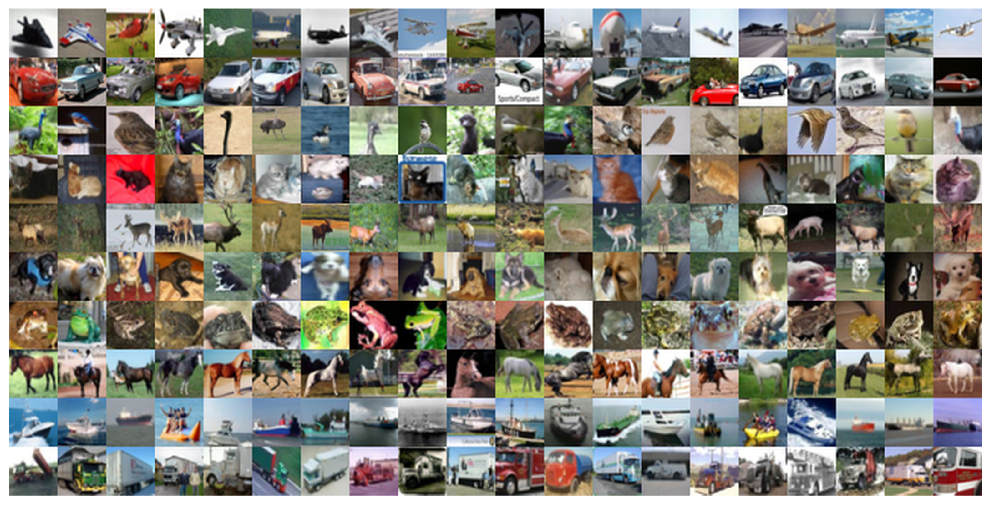
The CIFAR-10 dataset [30] holds significant importance within computer vision, encompassing a repository of 60,000 images. It serves as a rigorous evaluation platform for computer vision algorithms, with a primary focus on tasks. Figure 2 presents visual examples drawn from each of the ten object classes in the CIFAR-10 dataset. Additionally, Table 2 provides a detailed breakdown of the dataset’s category distribution, offering a comprehensive overview of the dataset’s composition. Apart from evaluating the model’s performance on the CIFAR-10 dataset, we conducted evaluations across the CIFAR-100 [30], MNIST [31], and Fashion-MNIST [32] datasets. This broader assessment enabled us to gauge the model’s generalizability across diverse image domains.

Figure 2.
Visual samples of CIFAR-10.
Table 2.
Distribution of categories in CIFAR-10 dataset.
4. Experiments
This section encompasses an in-depth exploration of the experimental setup, the environment details, hyperparameter influences, comparative analysis of proposed and plain blocks, and a comprehensive performance evaluation against SOTA models.
4.1. Experimental Environment
The experiments were conducted on a Linux operating system (version 5.4.0-132-generic) with an x86_64 CPU architecture. The setup comprises an Intel Xeon Platinum 8255C with 12 virtual CPUs and an NVIDIA GeForce RTX 3080 GPU. The CPU, manufactured by Intel, boasts significant computational capacity. The Python programming language (version 3.8.10) and the PyTorch deep learning framework (version 2.0.0+cu118) were used in this study, along with the TorchVision library (version 0.15.1+cu118).
4.2. Experimental Results
We conducted extensive experiments to investigate the influence of critical hyperparameters, including training epochs, learning rate, choice of optimizer, and data augmentation strategies. Through this rigorous experimentation, we aim to provide valuable empirical insights that can empower practitioners to make informed decisions regarding these crucial parameters, fostering more effective model training practices.
4.2.1. The Influence of Epochs
The model’s training outcomes are influenced by various hyperparameters, among which determining the appropriate number of “epochs” or training iterations is pivotal. Each epoch signifies one full pass of the model through the entire training dataset. During training, the model continuously adjusts its weights and biases to minimize the loss function. Therefore, the number of epochs directly affects how well the model learns from the data.
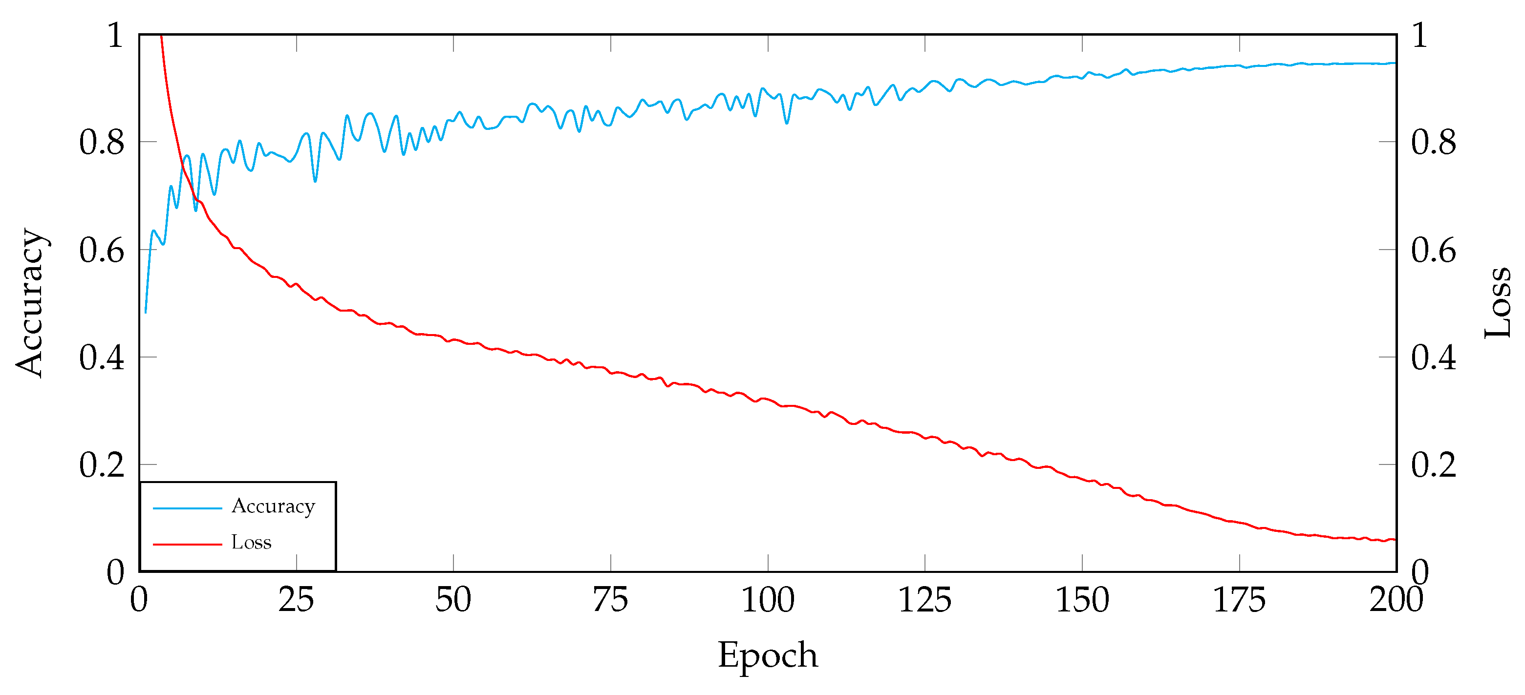
Based on the trends presented in Figure 3, the following observations can be made:
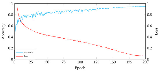
Figure 3.
The relationship between accuracy and training epochs.
- In the first approximately 25 rounds of training, the loss rapidly decreases, and the accuracy significantly improves.
- From the 25th round to roughly the 175th round, the loss continues to decrease, and the accuracy steadily increases.
- From the 175th round to approximately the 200th round, both the loss and accuracy gradually converge.
Setting the epoch size too small can lead to insufficient training, as the model may not have enough time to learn all of the patterns in the training data. This can result in poor performance on the test data. Setting the epoch size too large can lead to overfitting, as the model may learn the training data too well, including noise and irrelevant features. This can also result in poor performance on the test data.
Therefore, it is important to carefully consider the factors that affect epoch size selection, such as the size of the training dataset, the complexity of the model, and the risk of overfitting. In general, for smaller datasets, a smaller epoch size is recommended to avoid overfitting. For larger datasets, a larger epoch size may be necessary to fully learn the training data.
4.2.2. The Influence of Learning Rate
The learning rate directly influences the speed at which model parameters are updated, thereby having a profound impact on the model’s performance and convergence. To accurately assess the role of the learning rate, we employed the method of controlling variables. We ensured that all other hyperparameters, such as the training epoch, data transformation, optimizer, and batch size, were kept constant throughout our experiments. This allowed us to isolate the impact of the learning rate on model performance.
We conducted experiments using various learning rate values, specifically including 0.1, 0.01, 0.001, and 0.0001. By comparing how model performance varied with epoch under these different learning rates, we gained a more intuitive understanding of the pivotal role played by the learning rate during training.
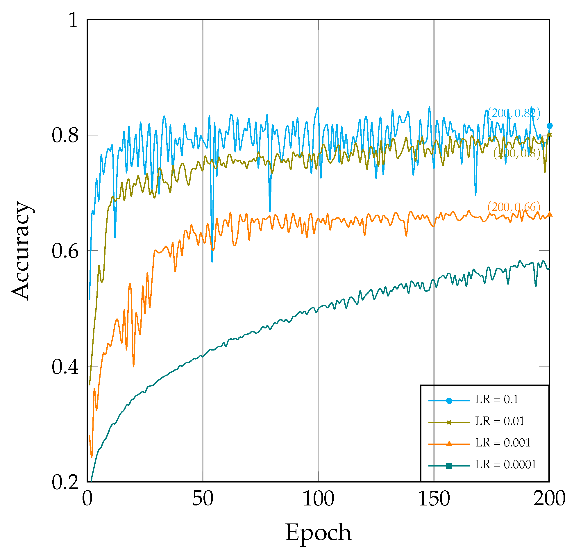
As illustrated in Figure 4, the learning rate has a significant impact on the model’s training process. Several observations can be made:
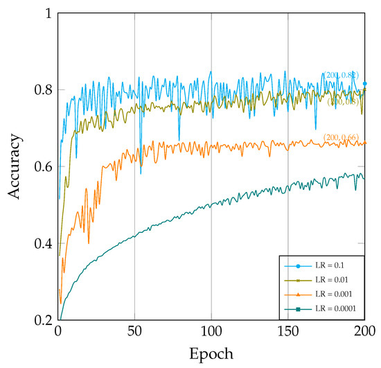
Figure 4.
The correlation between accuracy and epochs under varied learning rates.
- When the learning rate is set to a higher value (e.g., 0.1 in Figure 4), the model’s learning speed noticeably accelerates, leading to a rapid increase in accuracy. However, if the learning rate is set excessively high, it may lead to training oscillations and non-convergence and cause the model to miss the global optimum.
- Conversely, when the learning rate is set to a lower value(e.g., 0.0001 in Figure 4), the model’s learning speed slows down, resulting in a more stable training process. However, this can significantly slow down the convergence speed. Additionally, a smaller learning rate may cause the model to become stuck in a local optimum.
Therefore, the choice of learning rate necessitates a delicate balance between achieving rapid convergence and maintaining stability, allowing for comprehensive model training while avoiding the pitfalls of local optima.
4.2.3. The Influence of Optimizer
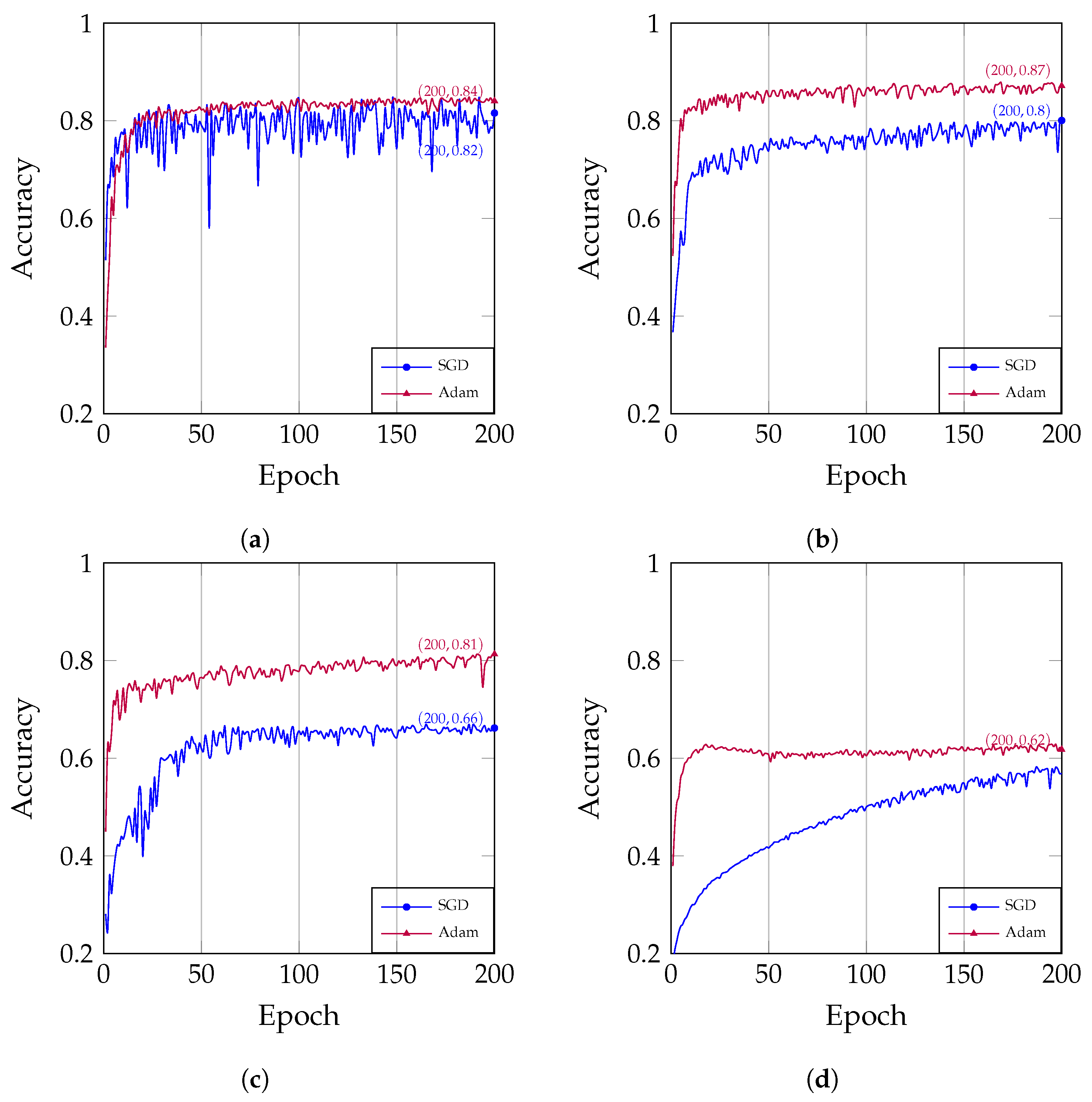
The choice of optimizer is a critical factor that influences the performance of model training. In this study, we evaluated the performance of two popular optimizers: stochastic gradient descent (SGD) and Adam. We compared the relationship between the number of training epochs and accuracy under different learning rates for SGD [33] and Adam [34].
As shown in Figure 5, the training curve of Adam is smoother than that of SGD, mainly due to the momentum mechanism it uses. Momentum can help the model overcome oscillations during training, making the training curve more stable. In addition, Adam is relatively simple to use and less sensitive to hyperparameters, making it easier to achieve good results. However, for large or noisy training datasets, SGD is more likely to converge. Overall, Adam is more suitable for most tasks and datasets.
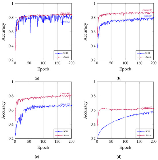
Figure 5.
The correlation between the number of epochs and accuracy under different optimizers: (a) The learning rate is set at 0.1; (b) The learning rate is set at 0.01; (c) The learning rate is set at 0.001. (d) The learning rate is set at 0.0001.
4.2.4. The Influence of Data Augmentation
Data augmentation strategies and transformations are pivotal during model training [35,36]. We examined the impact of various data augmentation methods, including random cropping, rotation, flipping, and more, on model performance. Our objective was to determine which data augmentation strategies contribute to enhanced model generalization and robustness.
This study investigated the following six data augmentation strategies:
- Baseline: Original data without any augmentation.
- Norm: Pixel values in training images are normalized to a standard distribution.
- HFlip: Randomly flip images horizontally.
- Crop: Randomly crop and pad images.
- Cutout: Randomly mask out a rectangular region in input images.
- All: Combines all of the above strategies.
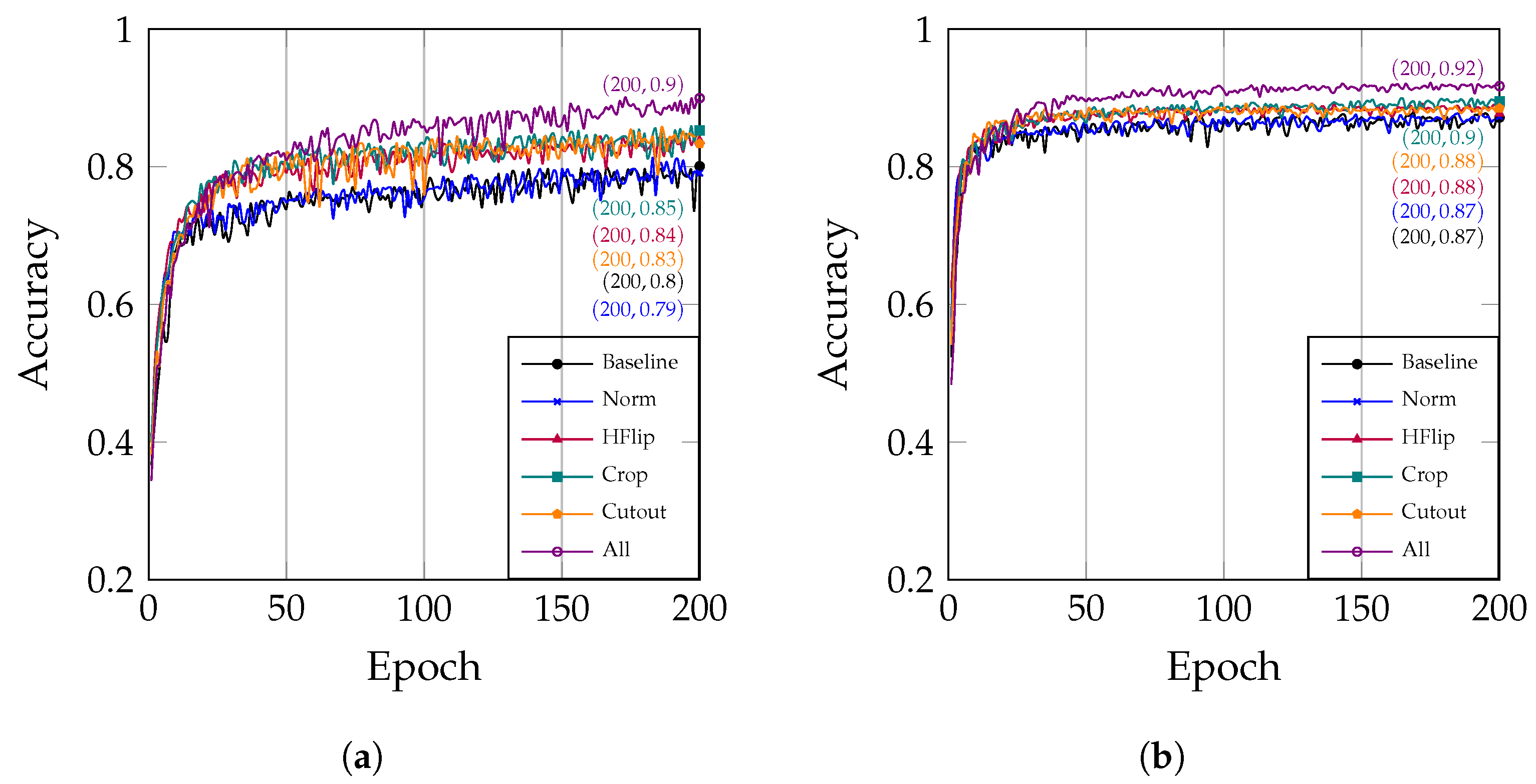
The experimental results indicate that data augmentation significantly enhances the model’s generalization ability and robustness.
Data normalization contributes to the stability of training, as evidenced by the blue curve (Norm) in Figure 6a. This curve is slightly smoother and exhibits less fluctuation than the black curve (Baseline), which corresponds to using the original data without any processing.
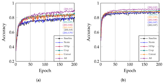
Figure 6.
The correlation between the number of epochs and accuracy under different data augmentation strategies: (a) The optimizer is set to SGD; (b) The optimizer is set to Adam.
Additionally, Figure 6a clearly shows that the data augmentation techniques (HFlip, Crop, and Cutout) have a positive impact on the model’s accuracy. Specifically, the accuracy reaches 0.84 after HFlip is applied, 0.85 after Crop is applied, and 0.83 after Cutout is applied. The most significant improvement in performance is observed when these data augmentation techniques are combined, resulting in an accuracy of 0.90. Analogously, Figure 6b demonstrates that data augmentation is also effective when using the Adam optimizer.
Data augmentation is a crucial technique for improving the performance of deep learning models. In practical applications, appropriate data augmentation strategies should be selected based on the characteristics of the data and the objectives of the task. By judiciously augmenting the data, we can effectively enhance the model’s generalization ability and robustness, thereby improving its performance in real-world applications.
4.3. Comparison between the MF Block and the Plain Block
In MF block (see Figure 7a), we set the 1 × 1 convolutional channel to 12, the first 3 × 3 convolutional channel is also 12, the second 3 × 3 convolutional channel is 6, and the third 3 × 3 convolutional channel is 6. In the MF block, these three convolutions are concatenated with the input, so with each passage through an MF block, the number of feature channels increases by 24 (12 + 6 + 6).

Figure 7.
(a) The MF block and (b) the plain block. The MF block and the plain block. To ensure that the network’s depth remains the same, we also set the number of convolutions in the compared plain block to four. In order to maintain consistent output features for each stage of the model, we set the number of channels in the last convolutional layer of the plain block to the number of channels in the previous feature map plus 24.
To elucidate the differences between the MF block and the plain block, we replaced the MF block in the model with the plain block (see Figure 7). Subsequently, we conducted a comparison between the two models and found that the model using the plain block was significantly more difficult to train (see Figure 8). The excessive number of convolutional layers primarily causes this difficulty, leading to issues such as gradient vanishing and exploding. These challenges exacerbate the problems during model training. In contrast, the MF block facilitated a smoother training process for the model and achieved superior results.
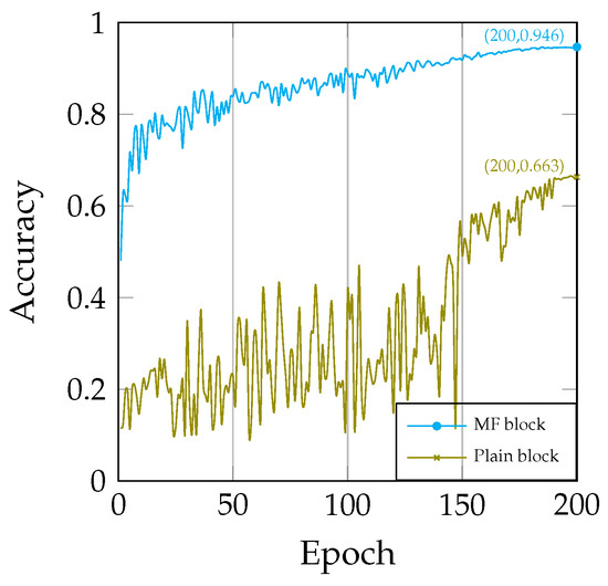
Figure 8.
Comparison of training: MF block vs. plain block.
Furthermore, we observed that the model employing the plain block had a parameter count of 0.78 M, despite having the same number of layers as our original model, which had a parameter count of 0.52 M. This indicates that the model, which utilizes the MF block, is more parameter-efficient, resulting in a higher parameter utilization rate.
4.4. Comparative Analysis with Other Models
We extensively validated the model across four distinct datasets: CIFAR-10, CIFAR-100, MNIST, and Fashion-MNIST. By validating the model on these four datasets, we were able to comprehensively assess its performance. The experimental results indicate that the model performed well across these datasets, showcasing its strong image classification capability, generalization, and robustness.
4.4.1. Performance on the CIFAR-10 Dataset
We conducted a comparative analysis between our proposed model and some classical models. As presented in Table 3, we observed a range of accuracy performances among the models, which varied from 92.31% to 95.04%. This variability is further explored in Figure 9. Notably, GoogLeNet and DenseNet121 demonstrated slightly higher levels of accuracy compared to the other models.
Table 3.
Model comparison of the CIFAR-10 dataset.
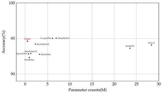
Figure 9.
Model comparison in terms of parameter count and accuracy on the CIFAR-10 dataset. Detailed comparisons are represented as shown in Table 3.
In contrast, our model surpassed these accuracy ranges by achieving an impressive accuracy of 94.60% while utilizing a significantly smaller parameter count of only 0.52 M. Remarkably, when compared to DenseNet121, our model required less than one-thirteenth of its parameters while experiencing only a marginal decrease in accuracy of 0.44%. This remarkable achievement is a result of our approach, which places equal emphasis on both high performance and parameter frugality. By prioritizing efficiency and resource optimization, our model proves to be an excellent choice for tasks with limited computational resources. The results unequivocally demonstrate the model’s effectiveness in striking a favorable balance between accuracy and efficiency.
Note that our model’s superior performance does not rely on additional datasets. This further reinforces the significance of our approach, as it showcases the model’s ability to excel without the need for extra data, making it even more valuable in practical applications.
4.4.2. Performance on the CIFAR-100 Dataset
To further evaluate the model’s performance, we conducted experiments on the CIFAR-100 dataset. The model achieved an accuracy of 75.82%, as depicted in Table 4. To accommodate the expanded range of 100 categories in CIFAR-100, the final fully connected layer of the model was correspondingly adjusted to 100 output neurons. This modification resulted in a total parameter count of 0.56 M for the model. CIFAR-100 comprises more categories, necessitating models to possess stronger discriminative and generalization capabilities. The experimental results indicate that the model maintains outstanding performance despite having significantly fewer parameters. Through experiments on these datasets, we further validated the effectiveness and broad applicability of the proposed model.
Table 4.
Model comparison on CIFAR-100 dataset.
4.4.3. Performance on the MNIST Dataset
The MNIST dataset is commonly used to evaluate models in relatively simple image classification tasks. Despite its simplicity, MNIST provides a benchmark for measuring a model’s ability to solve basic image classification problems. The model achieved an accuracy of 99.71% on MNIST with just 30 training rounds, demonstrating its capability in handling relatively straightforward image classification tasks. Note that most models can easily achieve over 99% accuracy on the MNIST dataset.
4.4.4. Performance on the Fashion-MNIST Dataset
Fashion-MNIST, characterized by more intricate image content compared to MNIST, closely simulates real-world applications. the model achieved an accuracy of 94.11% on the Fashion-MNIST dataset, and a comparison with SOTA models is presented in Table 5. These experiments enabled a deeper insight into the model’s proficiency in processing diverse and complex real-world images.
Table 5.
Model comparison on Fashion-MNIST dataset.
5. Conclusions
Lightweight models are significant for tasks such as image analysis, real-time image analysis, and defect detection on resource-constrained devices. In this paper, we propose a lightweight model with only 0.52 million parameters that achieves a 94.6% accuracy on the CIFAR-10 dataset. Our lightweight model was compared to SOTA models on the CIFAR-10 dataset. The model achieved superior accuracy under equivalent parameter conditions. Additionally, we conducted experiments on CIFAR-100, MNIST, and Fashion-MNIST datasets to validate the performance of the model. The MF block in LMFRNet effectively realizes feature reuse, thereby reducing the computational complexity of the model and improving its accuracy. Moreover, the model does not use residual blocks, which also provides an idea for exploring scenarios without residual blocks. Furthermore, to assist practitioners in understanding the hyperparameters used in our experiments, we conducted a comprehensive series of experiments to elucidate the roles of these hyperparameters and how to correctly configure them in practical applications.
In summary, the model maintains performance while having a very small parameter count, making it particularly amenable to resource-constrained domains or scenarios requiring real-time analysis. Future research directions based on our approach include:
- Extending our versatile classification model to a wider range of resource-constrained scenarios, such as Internet of Things (IoT) applications and embedded systems with limited computational resources.
- Investigating the use of the model as a backbone network for real-time object detection and other vision tasks, such as in autonomous vehicles, real-time crowd counting, and augmented reality environments.
To facilitate widespread utilization and advancement of the proposed model, we have made it open source (https://github.com/wgqhandsome/LMFRNet, accessed on 24 December 2023).
Author Contributions
Conceptualization, G.W.; Formal analysis, G.W.; Investigation, G.W.; Methodology, G.W.; Project administration, L.Y.; Resources, L.Y.; Software, G.W.; Supervision, L.Y.; Validation, G.W.; Visualization, G.W. and L.Y.; Writing—original draft preparation, G.W.; Writing—review and editing, L.Y. All authors have read and agreed to the published version of the manuscript.
Funding
This research received no external funding.
Data Availability Statement
The data presented in this study are openly available in [30].
Conflicts of Interest
The authors declare no conflicts of interest.
References
- Rawat, W.; Wang, Z. Deep Convolutional Neural Networks for Image Classification: A Comprehensive Review. Neural Comput. 2017, 29, 2352–2449. [Google Scholar] [CrossRef]
- Dhillon, A.; Verma, G.K. Convolutional Neural Network: A Review of Models, Methodologies and Applications to Object Detection. Prog. Artif. Intell. 2020, 9, 85–112. [Google Scholar] [CrossRef]
- Wang, Y.; Tian, Y. Exploring Zero-Shot Semantic Segmentation with No Supervision Leakage. Electronics 2023, 12, 3452. [Google Scholar] [CrossRef]
- Li, Z.; Liu, F.; Yang, W.; Peng, S.; Zhou, J. A Survey of Convolutional Neural Networks: Analysis, Applications, and Prospects. IEEE Trans. Neural Netw. Learn. Syst. 2021, 33, 6999–7019. [Google Scholar] [CrossRef]
- Savelli, B.; Bria, A.; Molinara, M.; Marrocco, C.; Tortorella, F. A Multi-Context CNN Ensemble for Small Lesion Detection. Artif. Intell. Med. 2020, 103, 101749. [Google Scholar] [CrossRef]
- Frid-Adar, M.; Diamant, I.; Klang, E.; Amitai, M.; Goldberger, J.; Greenspan, H. Modeling the Intra-class Variability for Liver Lesion Detection Using a Multi-class Patch-Based CNN. In Patch-Based Techniques in Medical Imaging; Wu, G., Munsell, B.C., Zhan, Y., Bai, W., Sanroma, G., Coupé, P., Eds.; Springer International Publishing: Cham, Switzerland, 2017; Volume 10530, pp. 129–137. [Google Scholar] [CrossRef]
- Bojarski, M.; Choromanska, A.; Choromanski, K.; Firner, B.; Ackel, L.J.; Muller, U.; Yeres, P.; Zieba, K. Visualbackprop: Efficient Visualization of Cnns for Autonomous Driving. In Proceedings of the 2018 IEEE International Conference on Robotics and Automation (ICRA), Brisbane, QLD, Australia, 21–25 May 2018; IEEE: Piscataway, NJ, USA, 2018; pp. 4701–4708. [Google Scholar]
- Coşkun, M.; Uçar, A.; Yildirim, Ö.; Demir, Y. Face Recognition Based on Convolutional Neural Network. In Proceedings of the 2017 International Conference on Modern Electrical and Energy Systems (MEES), Kremenchuk, Ukraine, 15–17 November 2017; IEEE: Piscataway, NJ, USA, 2017; pp. 376–379. [Google Scholar]
- Krizhevsky, A.; Sutskever, I.; Hinton, G. ImageNet Classification with Deep Convolutional Neural Networks. In Proceedings of the Advances in Neural Information Processing Systems, Lake Tahoe, NV, USA, 3–6 December 2012; Volume 2, pp. 1097–1105. [Google Scholar]
- Simonyan, K.; Zisserman, A. Very Deep Convolutional Networks for Large-Scale Image Recognition. arXiv 2015, arXiv:1409.1556. [Google Scholar]
- Szegedy, C.; Liu, W.; Jia, Y.; Sermanet, P.; Reed, S.; Anguelov, D.; Erhan, D.; Vanhoucke, V.; Rabinovich, A. Going Deeper with Convolutions. In Proceedings of the 2015 IEEE Conference on Computer Vision and Pattern Recognition (CVPR), Boston, MA, USA, 7–12 June 2015; pp. 1–9. [Google Scholar] [CrossRef]
- He, K.; Zhang, X.; Ren, S.; Sun, J. Deep Residual Learning for Image Recognition. In Proceedings of the 2016 IEEE Conference on Computer Vision and Pattern Recognition (CVPR), Las Vegas, NV, USA, 27–30 June 2016; pp. 770–778. [Google Scholar] [CrossRef]
- Huang, G.; Liu, Z.; Van Der Maaten, L.; Weinberger, K.Q. Densely Connected Convolutional Networks. In Proceedings of the 2017 IEEE Conference on Computer Vision and Pattern Recognition (CVPR), Honolulu, HI, USA, 21–26 July 2017; pp. 2261–2269. [Google Scholar] [CrossRef]
- Bhuiyan, M.A.B.; Abdullah, H.M.; Arman, S.E.; Rahman, S.S.; Al Mahmud, K. BananaSqueezeNet: A Very Fast, Lightweight Convolutional Neural Network for the Diagnosis of Three Prominent Banana Leaf Diseases. Smart Agric. Technol. 2023, 4, 100214. [Google Scholar] [CrossRef]
- Gu, M.; Zhang, Y.; Wen, Y.; Ai, G.; Zhang, H.; Wang, P.; Wang, G. A Lightweight Convolutional Neural Network Hardware Implementation for Wearable Heart Rate Anomaly Detection. Comput. Biol. Med. 2023, 155, 106623. [Google Scholar] [CrossRef] [PubMed]
- Ma, X.; Li, Y.; Wan, L.; Xu, Z.; Song, J.; Huang, J. Classification of Seed Corn Ears Based on Custom Lightweight Convolutional Neural Network and Improved Training Strategies. Eng. Appl. Artif. Intell. 2023, 120, 105936. [Google Scholar] [CrossRef]
- Zhang, D.; Hao, X.; Wang, D.; Qin, C.; Zhao, B.; Liang, L.; Liu, W. An Efficient Lightweight Convolutional Neural Network for Industrial Surface Defect Detection. Artif. Intell. Rev. 2023, 56, 10651–10677. [Google Scholar] [CrossRef]
- Iandola, F.N.; Han, S.; Moskewicz, M.W.; Ashraf, K.; Dally, W.J.; Keutzer, K. SqueezeNet: AlexNet-level Accuracy with 50x Fewer Parameters and <0.5 MB Model Size. arXiv 2016, arXiv:1602.07360. [Google Scholar] [CrossRef]
- Ma, N.; Zhang, X.; Zheng, H.T.; Sun, J. ShuffleNet V2: Practical Guidelines for Efficient CNN Architecture Design. arXiv 2018, arXiv:1807.11164. [Google Scholar] [CrossRef]
- Sandler, M.; Howard, A.; Zhu, M.; Zhmoginov, A.; Chen, L.C. MobileNetV2: Inverted Residuals and Linear Bottlenecks. arXiv 2019, arXiv:1801.04381. [Google Scholar] [CrossRef]
- Tan, M.; Le, Q.V. EfficientNet: Rethinking Model Scaling for Convolutional Neural Networks. arXiv 2020, arXiv:1905.11946. [Google Scholar] [CrossRef]
- Goodfellow, I.; Bengio, Y.; Courville, A. Deep Learning; MIT Press: Cambridge, MA, USA, 2016. [Google Scholar]
- Ioffe, S.; Szegedy, C. Batch Normalization: Accelerating Deep Network Training by Reducing Internal Covariate Shift. arXiv 2015, arXiv:1502.03167. [Google Scholar] [CrossRef]
- Xu, B.; Wang, N.; Chen, T.; Li, M. Empirical Evaluation of Rectified Activations in Convolutional Network. arXiv 2015, arXiv:1505.00853. [Google Scholar]
- He, K.; Zhang, X.; Ren, S.; Sun, J. Delving Deep into Rectifiers: Surpassing Human-Level Performance on ImageNet Classification. arXiv 2015, arXiv:1502.01852. [Google Scholar]
- Szegedy, C.; Vanhoucke, V.; Ioffe, S.; Shlens, J.; Wojna, Z. Rethinking the Inception Architecture for Computer Vision. In Proceedings of the IEEE Conference on Computer Vision and Pattern Recognition, Las Vegas, NV, USA, 27–30 June 2016; pp. 2818–2826. [Google Scholar]
- Szegedy, C.; Ioffe, S.; Vanhoucke, V.; Alemi, A. Inception-v4, Inception-ResNet and the Impact of Residual Connections on Learning. arXiv 2016, arXiv:1602.07261. [Google Scholar] [CrossRef]
- Wang, R.J.; Li, X.; Ling, C.X. Pelee: A Real-Time Object Detection System on Mobile Devices. arXiv 2019, arXiv:1804.06882. [Google Scholar]
- Ren, F.; Liu, W.; Wu, G. Feature Reuse Residual Networks for Insect Pest Recognition. IEEE Access 2019, 7, 122758–122768. [Google Scholar] [CrossRef]
- Krizhevsky, A.; Hinton, G. Learning Multiple Layers of Features from Tiny Images, Tech Report. 2009. Available online: https://www.cs.toronto.edu/~kriz/cifar.html (accessed on 24 December 2023).
- Lecun, Y.; Bottou, L.; Bengio, Y.; Haffner, P. Gradient-Based Learning Applied to Document Recognition. Proc. IEEE 1998, 86, 2278–2324. [Google Scholar] [CrossRef]
- Xiao, H.; Rasul, K.; Vollgraf, R. Fashion-MNIST: A Novel Image Dataset for Benchmarking Machine Learning Algorithms. arXiv 2017, arXiv:1708.07747. [Google Scholar]
- Robbins, H.; Monro, S. A Stochastic Approximation Method. Ann. Math. Stat. 1951, 22, 400–407. [Google Scholar] [CrossRef]
- Kingma, D.P.; Ba, J. Adam: A Method for Stochastic Optimization. arXiv 2017, arXiv:1412.6980. [Google Scholar] [CrossRef]
- Choi, H.; Park, J.; Yang, Y.M. A Novel Quick-Response Eigenface Analysis Scheme for Brain–Computer Interfaces. Sensors 2022, 22, 5860. [Google Scholar] [CrossRef] [PubMed]
- DeVries, T.; Taylor, G.W. Improved Regularization of Convolutional Neural Networks with Cutout. arXiv 2017, arXiv:1708.04552. [Google Scholar] [CrossRef]
- Zhang, X.; Zhou, X.; Lin, M.; Sun, J. ShuffleNet: An Extremely Efficient Convolutional Neural Network for Mobile Devices. In Proceedings of the 2018 IEEE/CVF Conference on Computer Vision and Pattern Recognition, Salt Lake City, UT, USA, 18–23 June 2018; pp. 6848–6856. [Google Scholar] [CrossRef]
- Howard, A.G.; Zhu, M.; Chen, B.; Kalenichenko, D.; Wang, W.; Weyand, T.; Andreetto, M.; Adam, H. MobileNets: Efficient Convolutional Neural Networks for Mobile Vision Applications. arXiv 2017, arXiv:1704.04861. [Google Scholar] [CrossRef]
- Dosovitskiy, A.; Beyer, L.; Kolesnikov, A.; Weissenborn, D.; Zhai, X.; Unterthiner, T.; Dehghani, M.; Minderer, M.; Heigold, G.; Gelly, S.; et al. An Image Is Worth 16 × 16 Words: Transformers for Image Recognition at Scale. arXiv 2021, arXiv:2010.11929. [Google Scholar] [CrossRef]
- Nocentini, O.; Kim, J.; Bashir, M.Z.; Cavallo, F. Image Classification Using Multiple Convolutional Neural Networks on the Fashion-MNIST Dataset. Sensors 2022, 22, 9544. [Google Scholar] [CrossRef]


Disclaimer/Publisher’s Note: The statements, opinions and data contained in all publications are solely those of the individual author(s) and contributor(s) and not of MDPI and/or the editor(s). MDPI and/or the editor(s) disclaim responsibility for any injury to people or property resulting from any ideas, methods, instructions or products referred to in the content. |
© 2023 by the authors. Licensee MDPI, Basel, Switzerland. This article is an open access article distributed under the terms and conditions of the Creative Commons Attribution (CC BY) license (https://creativecommons.org/licenses/by/4.0/).