Congestion Avoidance in Intelligent Transport Networks Based on WSN-IoT through Controlling Data Rate of Zigbee Protocol by Learning Automata

Abstract

Congestion control is one of the primary challenges in improving the performance of wireless sensor networks (WSNs). With the development of this network based on the Internet of Things (IoT), the importance of congestion control increases, and the need to provide more efficient strategies to deal with this problem is strongly felt. This problem is even more important in applications such as Intelligent Transport Systems (ITSs). This article introduces a new method for congestion control in ITSs based on WSN-IoT infrastructure, namely, the Congestion Avoidance by Reinforcement Learning algorithm (CARLA). The purpose of the research was to improve the performance of the Zigbee protocol in congestion control through more efficient routing and also the intelligent adjustment of the data rate of the nodes. For this purpose, a topology control and routing strategy based on the multiple Bloom filter (MBF) is proposed in this research. Further, learning automata (LA) was used as a reinforcement learning model to adjust the data rate of network nodes in a distributed manner. These strategies distinguish the current research from previous efforts and can be effective in reducing the probability of congestion in the network. The performance evaluation results of the proposed algorithm in a simulated ITS environment were compared with conventional Zigbee and state of the art methods. According to the results, CARLA can improve PDR by 4.64%, and at the same time, reduce energy consumption and end-to-end delay by 11.44% and 25.26%, respectively. The results confirm that by using CARLA, in addition to congestion control in the ITS, energy consumption and the end-to-end delay can also be reduced.

1. Introduction

In recent years, WSNs have played a vital role in various fields. A WSN consists of a large number of sensor nodes. These sensor nodes acquire real-time information and transmit the information [1]. When a large number of sensor nodes are active in transmitting information, there is a possibility of congestion in data packets [2]. Congestion occurs due to buffer overflow, channel contention, packet collision, and wireless channel state change. Congestion has a direct impact on efficiency and quality of service [3]. With the introduction of IoT structure and the architectures for WSNs based on the infrastructure of IoT, the issue of congestion control has become more important [4] because the infrastructure of IoT provides the possibility of forming WSNs with a much larger number of heterogeneous things in wider areas, which enables these networks to be used in applications such as ITSs [5]. This situation means an increase in the probability of congestion in different areas of the network [6,7]. Two types of congestion can occur in an ITS based on WSN-IoT. The first type is node-level congestion, which is caused by the buffer overflow in the node and can cause the loss of packets and increase the queuing delay. The second type is link-level congestion, which is related to the wireless channel shared by several nodes [8]. There are different methods to detect and resolve congestion in wireless networks. Algorithms based on data priority, delivery ratio, congestion avoidance, and routing have been presented [9]. One of the congestion control methods is changing the data transmission rate of network nodes. In these algorithms, when congestion is detected in an area, the data rate of the nodes responsible for the congestion is changed to improve the network performance. Yet, it should be noted that changing the data rate of the network nodes without considering the global parameters of the network (such as the transmit rate of neighbors, the number of packets in progress, etc.) will reduce the operational capacity and delivery rate of packets in the network, and this may downgrade the Quality of Service (QoS) in intelligent transport networks [10]. Therefore, RL-based solutions can be suitable for achieving this goal by considering the global parameters of the environment. In this solution, the learning agent continuously interacts with the environment and corrects its decisions after receiving the response from the environment. One of the efficient methods of RL is LA. In this article, LA is used as a model to control the data rate of each thing in a distributed manner. The contributions of the current article include the following:

• In the method proposed in this article, a new mechanism based on LA is used to determine the appropriate data rate of each active network node among working rates of the Zigbee protocol. This model specifies the optimal strategy for determining the data rate of things by considering the behavioral criteria of nodes in the routing process. This mechanism, by using reward and penalty operators, can determine the optimal data rate for each active node of the intelligent transport network in an adaptable manner and in accordance with the behavior of the things.
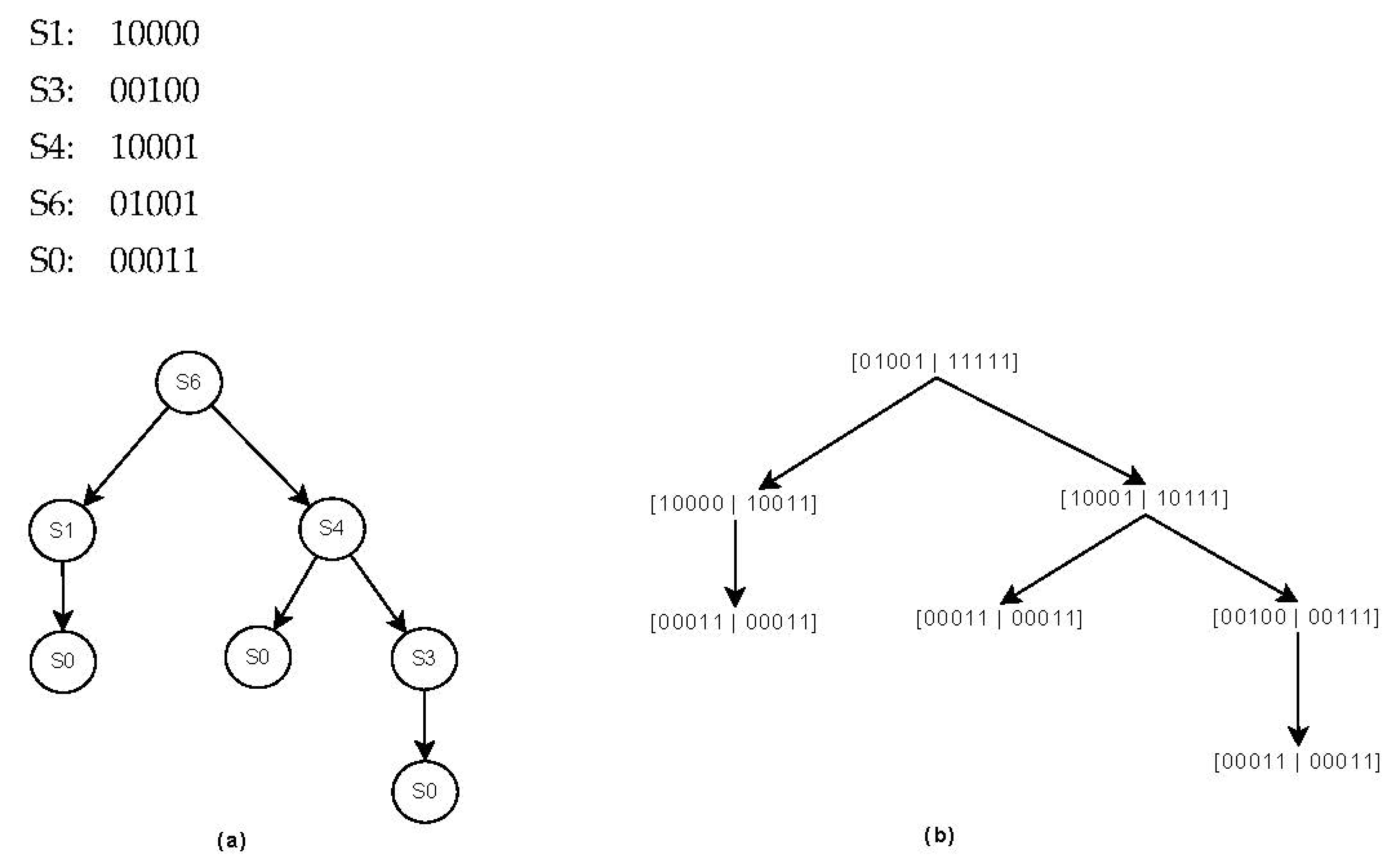
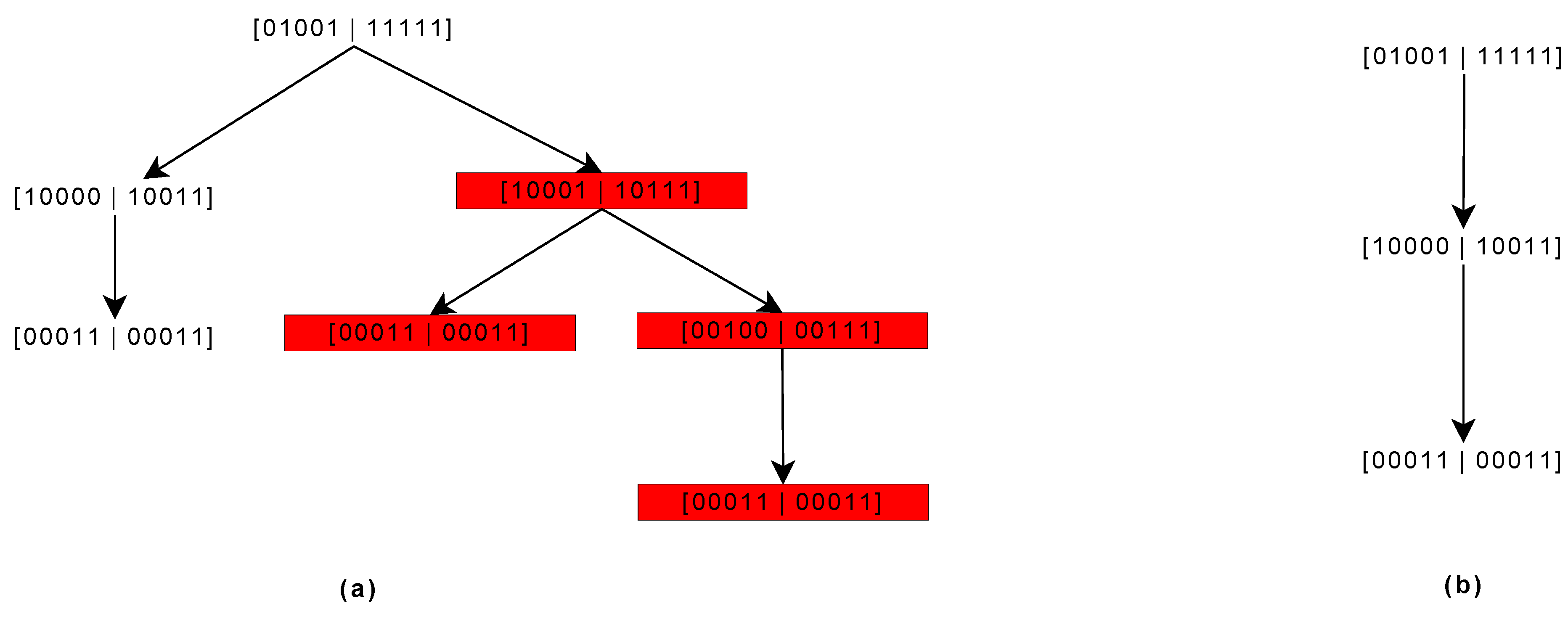
• This research provides an efficient solution to form the communication platform of nodes in transport networks based on WSN-IoT infrastructure. This method is a hierarchical and low-cost communication structure, based on MBF, which checks the existence of the path only by performing a few bit comparisons. In this method, the value of the existing routes is also determined based on the functional criteria of the objects. This structure can manage nodes with low energy at the lowest cost and provide a mechanism to form alternative paths for each node to reach its destination.

Since the mentioned cases have not been studied in previous works, these cases can be considered as innovations of the current research. The remainder of the paper is organized as follows: The Section 2 reviews related studies about congestion control in WSN-IoT. In the Section 3, CARLA is described in details. In the Section 4, the efficiency of CARLA is evaluated from different aspects. Finally, in the Section 5, conclusions are made and limitations of the research are described.

2. Related Works

Congestion avoidance has always been one of the topics of interest for researchers in the field of IoT and WSNs, and the reason for this is the challenging nature of this problem in networks with wide dimensions and dynamic structures. In this section, some of the recent efforts to control and avoid congestion in IoT-based WSNs are reviewed.

In [11], a method to control the traffic congestion of IoT in environmental applications was presented. The method presented in this article is a multipath clustering and routing protocol based on load balance for heterogeneous WSNs (HWSNs) that can be used in the context of IoT. The selection of the cluster head nodes to form the clustering structure of the network was implemented using the criteria of the remaining energy and the number of neighbors. Moreover, the routing algorithm presented in this method levels the cluster head nodes based on the distance from the base station and determines the routes for each cluster to reach the destination based on the number of determined levels. The criteria used for cluster formation and route selection in this method may lead to the immediate draining of energy resources in regions with a high traffic load, such as areas near the base station.

In [12], a congestion control algorithm for IoT-based WSNs was presented, which uses machine learning (ML) techniques. This method includes two main steps: In the first step, the transmitting window size of packets is predicted using ML techniques. Then, in the second step, the data packets are classified into priority packets and normal packets and are sent within the allocated window size. This method faces difficulties in implementation, because training the learning model in a network through this method requires having data collected through the operations of the same network.

In [13], a strategy based on ML was introduced to detect congestion in IoT-based WSNs. The learning strategy used in this method is a Support Vector Machine (SVM). Its learning parameters are optimized using the squirrel search algorithm. In [14], a similar strategy was used to predict the congestion situation in IoT-based WSNs. This method uses the Artificial Flora (AF) algorithm to optimize the parameters of the SVM. In this method, criteria such as queue length, packet loss rate, and congestion queue size are received as inputs to the SVM, and this learning model predicts the congestion situation based on the mentioned criteria. Based on the anticipated congestion situation, a decision is made in the context of offloading the node to the server. The methods in [13,14] suffer the same problem as the method presented in [12], and it is difficult to collect the training data to construct the SVM models for different network configurations. On the other hand, due to the time-consuming process of SVM optimization, this operation should be executed offline; however, this process requires online network data.

In [15], a Collision-Aware Routing algorithm using a Multi-Objective Seagull Optimization Algorithm (CAR-MOSOA) was presented to improve the efficiency and scalability of WSNs. CAR-MOSOA uses a clustering approach for improving the scalability of the network and uses MOSOA to select network cluster heads, and the routing process is performed in a multi-hop manner through cluster head nodes. In this method, CH selection is performed using parameters such as coverage, communication cost, residual energy and degree of nodes. Further, the route selection is performed using the queue length and link quality of discovered paths. This algorithm has problems, such as a high computational complexity and lack of distributability, which leads to high latency in large-scale networks.

In [16], a Distributed Congestion Control Protocol (DCCP) was presented for congestion control and end-to-end delay improvement in WSNs. In this method, congestion is first detected using two indicators. Then, each node collects the received data and creates a traffic density map, which is used to calculate the best route. Using this approach can be effective in improving the traffic balance on routes and reducing end-to-end delay. In this method, a data rate control scheme is used to prevent congestion in the network by sending a congestion notification message to a source node. This mechanism uses static threshold values for detecting congestion and classifies nodes into three states: normal, slow, and urgent. The data rate of each node is determined using these states, but may lead to a high packet overhead. On the other hand, using a reactive mechanism for congestion control in this algorithm causes the nodes’ buffer to fill quickly.

In [17], a green hybrid congestion control mechanism for IoT-based WSNs is presented. This method uses an unequal clustering mechanism that saves the energy of sensor nodes. Moreover, in this method, a congestion avoidance mechanism based on data prioritization is used, which can be effective in reducing delay. The clustering strategy used in this method requires each node to know its position, based on which the cost of implementing the model increases. Further, the technique of data prioritization in this method requires the analysis of the content of packets, which can lead to privacy violations and an increase in complexity. The method proposed in [18] is a dynamic routing algorithm based on the shortest path using the Optimal Link-State Routing (OLSR) strategy, which is modified to minimize communication delay. This method uses a strategy to find the shortest alternative path when the communication between two nodes fails. Additionally, this method uses a congestion avoidance scheme that is effective in reducing the communication delay of nodes. However, this method has not been able to solve some of the problems of the OLSR method, such as the high number of control packets in cases of link failure, or the quality of service reduction in conditions of increased network density.

In [19], an adaptive algorithm for the congestion window in IoT was introduced. This algorithm can adapt to network traffic conditions, and its goal is to increase throughput and reduce delay while avoiding congestion in the network. Thus, in this method, the size of the congestion window depends on criteria such as the source transmit rate, route bandwidth, and receiver delivery ratio. In [20], the combination of clustering and optimization techniques was used for congestion control in WSNs. In this method, the combination of K-Means clustering and the greedy search algorithm was used for clustering network nodes. Moreover, the firefly optimization algorithm was used to determine the optimal data rate of the nodes. Finally, data routing was based on the ant colony optimization algorithm. The use of the mentioned algorithms caused this method to have high computational complexity, which makes it unsuitable for large-scale networks. On the other hand, the equal clustering strategy used in this method leads to rapid energy loss in the nodes/clusters adjacent to the base station.

In [21], the application of two ML models, i.e., Artificial Neural Network (ANN) and SVM, was studied to predict the state of node congestion in WSNs. The parameters used in these learning models to predict the congestion situation were the number of sensor nodes, the traffic rate, and node retention. The results of comparing these two methods showed that the artificial neural network can predict the congestion situation with higher accuracy. However, this research has not provided a solution to automatically generate training data for learning models that can be used dynamically in different network configurations.

3. Proposed Model (CARLA)

In this section, the proposed algorithm for congestion avoidance in transport networks based on WSN-IoT is explained. CARLA tries to control network congestion by providing a new structure for network topology control. This algorithm, by providing a data rate control solution in the network, in addition to creating reliable routes for data exchange, minimizes the computational load of each node for optimal routing. The great advantage of CARLA can be considered the simplicity of the calculations and its optimal performance in determining the route and choosing the appropriate data rate for things. This algorithm uses LA to determine the data rate in each node. CARLA is based on the following assumptions:

• The strength of the received signal in a wireless communication has a direct relationship with the distance between the transmitter and the receiver. Therefore, the distances between the nodes can be estimated through the strength of the received signal.
• The deployment of sensor nodes in the network environment is random and uniform. Further, the density of sensor nodes in different areas of the environment is almost uniform. Some network nodes have mobility capabilities; therefore, the assumed network structure changes dynamically.
• The characteristics of each thing (such as initial energy, buffer memory capacity, etc.) can be different from other things. Therefore, the assumed network is heterogeneous. When the remaining energy of a node reaches one percent of its initial energy, the node notifies its neighbors of its energy depletion by broadcasting a message about reducing energy consumption. As a result, the node with low energy will be removed.
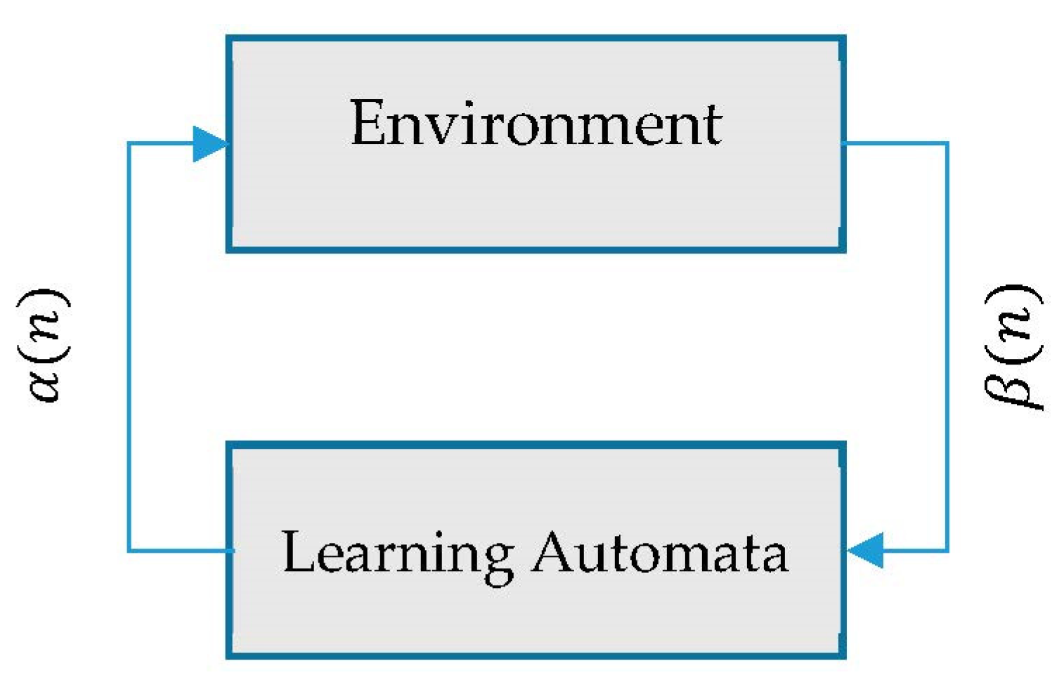
• Each sensor node in the network is equipped with an automata unit, which is used to determine the appropriate data rate for that node.

CARLA tries to improve the performance of the transport networks in the face of congestion by controlling a simple and fault-tolerant topology. Based on this, CARLA can be summarized in four main steps:

(1)

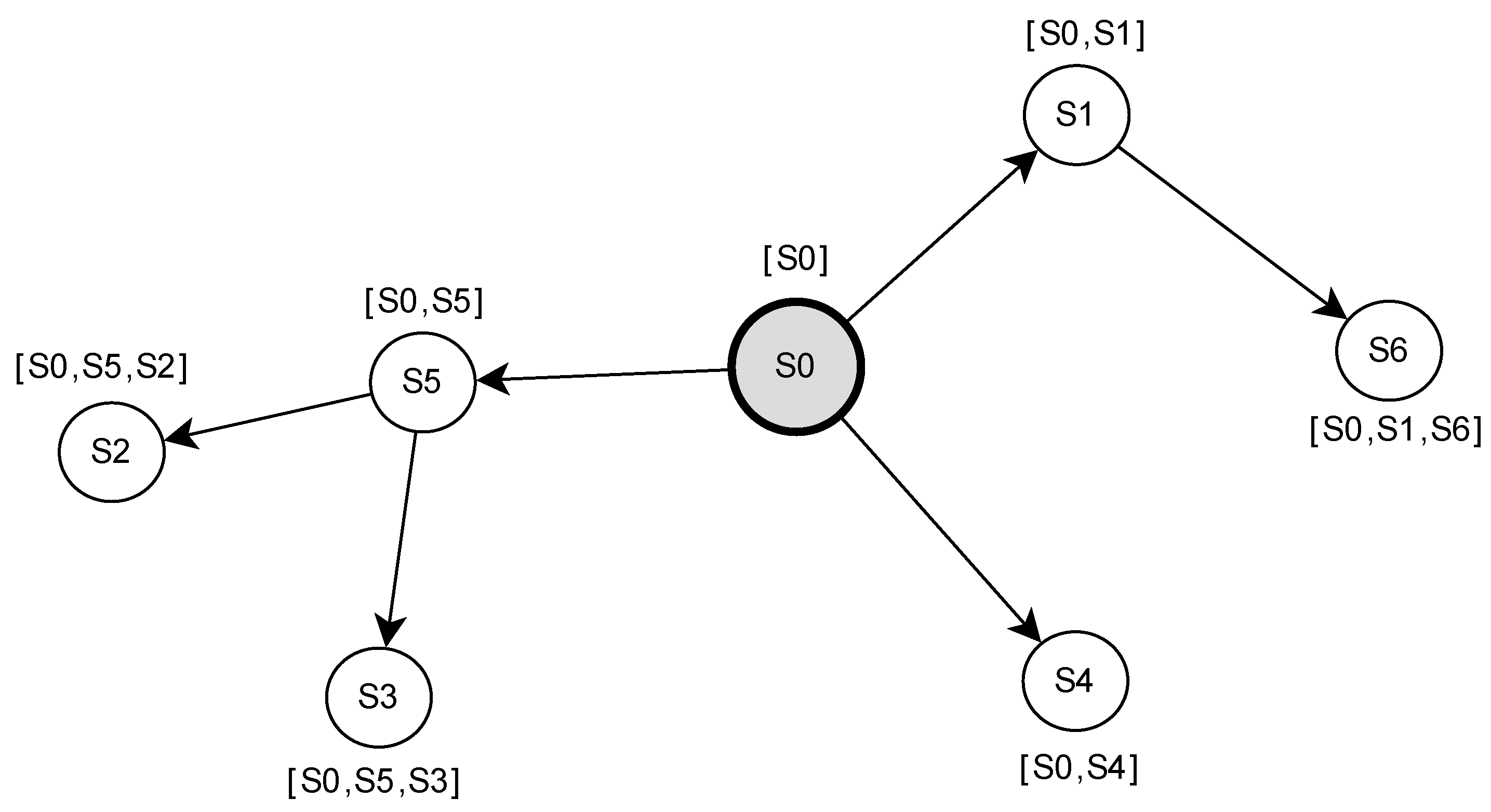
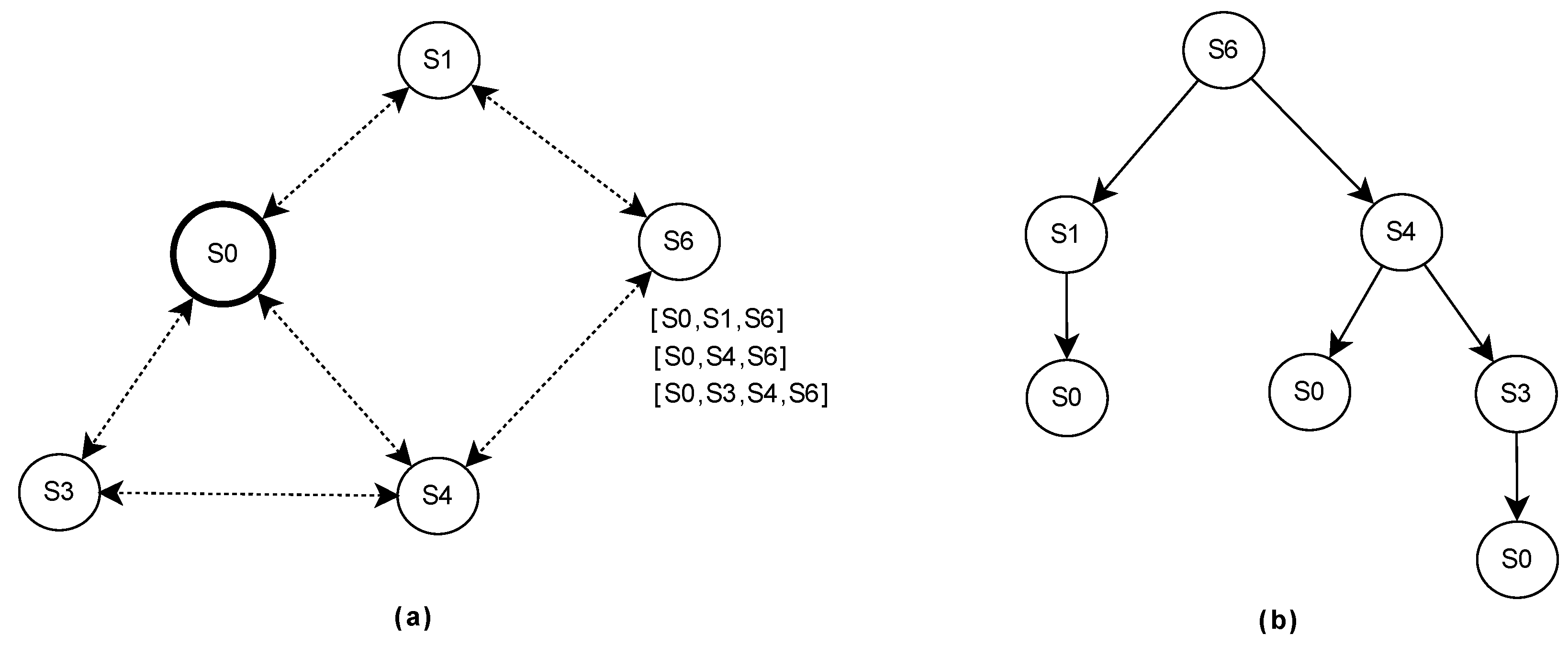
Topology control (construction and control of hierarchical local tree in each node);

(2)

Management of nodes with low energy level;

(3)

Data rate control using LA;

(4)

Local hierarchical tree-based routing.

These steps are explained in the following.

3.1. Topology Control

The topology construction and control step is the first and most important step in the performance of CARLA. Although the Zigbee protocol involves strategies for routing in the network, these methods have deficiencies that make them inefficient for use in large networks, such as transport networks. Routing in Zigbee depends on the network topology. The routing algorithm based on hierarchical topology in this protocol supports only 10 hops. On the other hand, the lack of scalability and instability in wide networks are some other disadvantages of the Zigbee routing algorithms. For this reason, in CARLA, an efficient solution for topology control and routing is provided, which solves the shortcomings of the Zigbee protocol.

In the proposed algorithm, each node will know its position relative to its neighbors and the destination node and will be able to generate a hierarchical structure of routes leading to the destination node. In this step, first, the base station starts the network topology construction operation by broadcasting a topology construction packet to all its neighboring nodes. The structure of this packet is shown in Figure 1.

The structure of this packet is based on IEEE 802.11 standards [22]. The Routing Data section in this data packet stores the information of intermediate nodes in the routes traveled by each packet. This part of the topology-forming packet is a list, and every node that receives this packet for the first time adds its address to the end of the list and rebroadcasts it to its neighbors. Figure 2 shows how the routing data section is formed from the node that creates the topology to other nodes in a sample network.

In Figure 2, the content of routing data sent by each node is displayed as a list next to that node. In CARLA, each node will use a tree structure to route data to the destination to control the network topology. This tree structure is based on MBF [23] and is explained below.

Upon receiving each packet, the topology is formed by a node, and the process of updating the MBF is performed. In addition to storing the address of each node, this filter maintains the network topology as a tree. The nodes of this tree represent the nodes of the network. The root of the structure formed in each node represents the node itself, and all the leaves of this structure represent the nodes that can be reached through the routes in the tree. As mentioned, the topology formation is initiated by the base station node through the broadcast of a packet. Each packet flowing during this step contains a route starting from this node and leading to different nodes. Therefore, each network node receives a topology formation packet and receives the information of a new route to the destination. This information is used to form and update the hierarchical structure based on the MBF located in each network node. The process of updating the hierarchical structure of the Bloom filter (BF) is achieved by sequentially picking addresses from the end of the list in the received packet. The last address in the list is added as a direct child of the current node, and other addresses in the list are added to the tree as nodes of lower levels. Figure 3 shows how this structure is formed in a sample network.

In Figure 3a, the S6 node receives three different packets during the topology construction process. Each of these packets provides the information of a new route to the destination S0 at the disposal of the S6 node. Based on these routes and using the described process, the S6 node forms a local hierarchical structure for the discovered routes; this tree structure is shown in Figure 3b. The root of the formed tree is node S6, and the leaves of the hierarchical tree lead to node S0. In the next step, the formed hierarchical structure will be transformed into an MBF. The discussed BF is a hierarchical tree structure, each node of which is a BF. The structure of each BF node consists of two parts, which are [A|B]. Part A stores the binary value of the hash code of the node’s address, and part B stores the hierarchical address of the BF based on the hash function. The B part of each BF is created through a bitwise OR operation on the A part of the current BF and its children. For example, if the address of each of the nodes in Figure 3, after applying the hash function, is as follows, the corresponding MBF is shown in Figure 4.

In Figure 4b, the root node is equivalent to node S6 in Figure 4a. As mentioned, all the Bloom nodes of the multiple filters have a bipartite structure, [A|B]. Part A is equivalent to the hash code of the node address, and part B is obtained by performing a bitwise OR operation between part B of the child nodes and part A of the node itself. As an example, for part B, we have the root node in Figure 4b:

$$\begin{array}{c} 10011\\ \mathrm{OR} 10011\\ \mathrm{OR} 01001\\ ------\\ = 11111\end{array}$$

(1)

This process starts hierarchically from the leaves of the tree and ends at the root node of the MBF.

3.2. Management of Nodes with Low Energy

In order to manage nodes with low energy, whenever the energy level of a node reaches a threshold value (1% of the initial energy), that node will broadcast an energy depletion message to its neighbors to inform them that it is running out of energy. Upon receiving this message, each neighboring node removes the low-energy node from its MBF and updates the changed branch. During the update process, all children of the low-energy node in the MBF structure are removed. Figure 5 shows the MBF structure of node S6 after the energy of node S4 is exhausted. It should be noted that, if all the connections of the node are removed, the mentioned node will broadcast a control message, so that if there is an active node in its neighborhood, it will receive the MBF structure of the neighboring node and complete its communications based on it.

3.3. Data Rate Control Using LA

In order to manage the load distribution in the network, in CARLA, the LA model is used to control the data rate of each node in the network. The use of LA makes the proposed model adjust its parameters based on the network structure after several iterations and selects the optimal action to reduce congestion in the network. The operation of determining the data rate of the nodes via LA in CARLA is performed periodically and every time the network topology structure is formed or updated. In the following, the method of determining the data rate via LA in each node is explained. Determining the data rate of each node in CARLA is achieved by using LA and by calculating the amount of data transmission rate changes for each node locally. The purpose of the presented model is to select the most appropriate data rate for each node according to the communication and positional characteristics of the node so that network congestion can be controlled. The structure of the automata used in CARLA is shown in Figure 6.

As shown in Figure 6, each LA works based on its interaction with the environment (network). The working process of LA is based on an iterative mechanism, in which at the beginning of each iteration, an action (shown as$\alpha \left(n\right)$ in Figure 6) is selected by LA and applied to the environmental components (network nodes). Then, the LA model receives the response of the environment (shown as$\beta \left(n\right)$ in Figure 6) in relation to its selected action, and based on the quality of the response, it updates the recently selected action using reward and penalty operators. Thus, each LA model has a set of actions to choose from. This set is named$\mathit{A} = \left\{{\mathbf{\alpha }}_{\mathbf{1}},{\mathbf{\alpha }}_{\mathbf{2}}, \dots ,{\mathbf{\alpha }}_{\mathit{n}}\right\}$. Each action in set A can be selected based on the set of possibilities. During this process, the automata learn to choose the optimal action by adjusting the probability of actions based on reward and penalty operations.

In CARLA, the actions set of each LA is defined as the working data rates of the Zigbee protocol, as follows:

$$\mathit{A}\mathbf{=}\left\{\mathbf{20},\mathbf{40},\mathbf{100},\mathbf{250}\right\}$$

(1)

In the above set, each action determines one of the working data rates of the Zigbee protocol, in kilobits per second. At the beginning of the network, considering the number of selectable actions N = 4, the probability of all the actions in the automata is 1/4. In this case, when all the actions have the same probability, the LA chooses one of its actions randomly. The set of automata possibilities is displayed as ${\mathit{P}}_{\mathit{LA}}=\left\{{\mathit{p}}_{\mathit{i}},{\mathit{p}}_{\mathbf{2}},\dots ,{\mathit{p}}_{\mathit{n}}\right\}$. In CARLA, each node periodically determines its sending rate using this model. In this way, the node first selects the action with the highest probability in its automata model and adjusts its data rate based on this action. It should be noted that the data rate is always determined as one of the working rates of the Zigbee protocol and within the allowed range $\left[\mathit{r}\mathit{a}\mathit{t}{\mathit{e}}_{\mathit{min}},\mathit{r}\mathit{a}\mathit{t}{\mathit{e}}_{\mathit{max}}\right]$. After determining the data rate, the routing operation is achieved based on the topology structure and the created data rate. After each sending period, the LA located in each node evaluates the response of the environment and updates its probability vector based on this response. In the following, this step of CARLA is explained.

3.4. Routing Based on Local Hierarchical Tree

In this section, the mechanism of the data packet routing phase using the proposed algorithm is described. Routing data packets from the source nodes to the base station is achieved only based on the local hierarchical tree formed in the topology control phase. The proposed structure for topology formation in CARLA increases the speed of the route search. For example, if we want to know whether there is a route between the root node and S3 in Figure 4, this operation is implemented by comparing the hash code of the B part of the root node with the hash code of the destination node. Hash code B for root node S6 is 11111. The hash code of the S3 node is 00100. We see that all the 1 bits of the S3 hash code are also 1 in the hash code of the root node; thus, there is a route from S6 to S3. To search the complete route and choose the next step to send data from S6 to S3, we compare the part B hash code of each S6 child node with the hash code of S3. For example, by comparing the hash part B code of the root left child (10011) with the hash code of S3 (00100), we see that in the hash code of S3, the third bit has a value of 1, but in 10011, this bit is zero. Therefore, it is definitely impossible to reach node S3 from this route. Yet, by comparing the right child, we find that this node reaches S3. Finally, repeating the operation at different levels determines that the desired route is S6-S4-S3. The described process is used to route data between network nodes. The flowchart related to the local algorithm for the route search using the proposed method is shown in Figure 7.

In the formed topology structure, each edge of the hierarchical tree is weighted based on the criteria of the remaining energy, occupied buffer rate, and successful transmission rate, such that if there are multiple routes between the source and the destination, routes with higher efficiency are selected for data transmission. To weigh the existing edge between two nodes, I and j, in the hierarchical tree, the following relationship is used:

$${\mathit{W}}_{\mathit{i}\mathit{j}}=\frac{{\mathit{b}}_{\mathit{j}}}{{\mathit{E}}_{\mathit{j}}\times \mathit{r}\mathit{a}\mathit{t}\mathit{i}{\mathit{o}}_{\mathit{j}}}$$

(2)

where b_j is the buffer occupancy factor of node j, and Equation (3) is used to calculate it.

$${\mathit{b}}_{\mathit{j}}=\frac{\mathit{bufferLeve}{\mathit{l}}_{\mathit{j}}}{\mathit{bufferCapacit}{\mathit{y}}_{\mathit{j}}}$$

(3)

Further, E_j is the remaining energy coefficient of node j and is calculated as follows:

$${\mathit{E}}_{\mathit{j}}=\frac{\mathit{EnergyLeve}{\mathit{l}}_{\mathit{j}}}{\mathit{InitialEnerg}{\mathit{y}}_{\mathit{j}}}$$

(4)

In Equation (2), ratio j represents the rate of successful packet routing by node j and is calculated as a ratio between the number of successfully routed packets and the number of packets received at node j. Each downstream node loads the parameters of the buffer occupancy coefficient, energy coefficient, and successful transmission rate of its respective packet on the ACK packets to be received by the upstream nodes. After performing the routing operation, the selection evaluation operation is performed in the LA of each node. In this step, each LA evaluates its previously selected action using the response received from the environment and will update its probability using reward and penalty operations. In the following, we explain how to perform this operation in CARLA.

3.5. Updating Automata Actions at the end of Each Round of the Cycle

As mentioned in the previous sections, the set of probabilities related to each action of the LA is used to determine the data rate for each node in the network. At the beginning of automata, the probability of all actions is equal. If the actions probabilities of the LA are the same, the automata choose one of the actions randomly. During the activity of the network, according to the actions selected by the automata and the responses received from the environment, reward and penalty rules are applied to the choices of the automata. Reward and penalty operations are performed at the end of each period and before determining the new data rate for network nodes. The reward and penalty rules for updating the set of automata possibilities are as follows.

• If at the end of a cycle, the rate of successful packet delivery by the node in the completed cycle is higher than the rate of successful packet delivery by the node in the previous cycles, the selected rate for the node in the last cycle is considered an optimal action. In this case, the probability of choosing it will also increase with the reward of the action related to this rate.
• If at the end of a cycle, the rate of successful packet delivery by the node in the completed cycle is lower than the rate of successful packet delivery by the node in the previous cycles, the selected rate for the node in the last cycle is considered a wrong action. In this case, the probability of choosing it will decrease with the penalty for this rate.

In the case of reward for the i-th action in the LA, the set of probabilities corresponding to each action of that automata is updated using the following relations [24]:

$${\mathit{p}}_{\mathit{j}}\left(\mathit{k}+\mathbf{1}\right)=\{\begin{array}{c}{\mathit{p}}_{\mathit{j}}\left(\mathit{k}\right)+\mathit{a}\left[\mathbf{1}-{\mathit{p}}_{\mathit{j}}\left(\mathit{k}\right)\right] \mathit{j}=\mathit{i},\\ \left(\mathbf{1}-\mathit{a}\right){\mathit{p}}_{\mathit{j}}\left(\mathit{k}\right) \forall \mathit{j}\ne \mathit{i}.\end{array}$$

(5)

where i is the number of the rewarded action, p is the set of probabilities corresponding to automata actions, and parameter $\mathit{a}$ is the reward coefficient. Actually, Equation (5) increases the probability of the rewarded action by the first relation and decreases the probability of other actions by the second relation.

If the i-th action is penalized in the automata, the set of probabilities corresponding to each action of that automata is updated using the following relations [24]:

$${\mathit{p}}_{\mathit{j}}\left(\mathit{k}+\mathbf{1}\right)=\{\begin{array}{c}\left(\mathbf{1}-\mathit{b}\right){\mathit{p}}_{\mathit{j}}\left(\mathit{k}\right) \mathit{j}=\mathit{i},\\ \left(\frac{\mathit{b}}{\mathit{r}-\mathbf{1}}\right)+\left(\mathbf{1}-\mathit{b}\right){\mathit{p}}_{\mathit{j}}\left(\mathit{k}\right) \forall \mathit{j}\ne \mathit{i}.\end{array}$$

(6)

where $\mathit{r}$ is the number of actions in the automata, and $\mathit{b}$ is the penalty coefficient of the actions. In fact, Equation (6) decreases the probability of penalized actions by the first relation and increases the probability of other actions by the second relation. Using this model’s causes in every reward and penalty operation, and selection by LA, the probability of optimal actions increases, and the LA can make more optimal decisions to determine the data rate. It should be noted that the value of reward and penalty coefficients (Equations (5) and (6)) should be set experimentally. The features of the presented model are its simplicity and ability to increase the accuracy of automata in determining the data rate by increasing the number of cycles in the network.

3.6. Complexity of CARLA

In order to calculate the complexity of the proposed method, the complexity of each of its steps should be checked. These steps include topology construction, MBF structure formation, route search, data rate control, and updating LAs. The complexity of the topology construction step in a network with N nodes is O (N), which is the result of transmitting N control packets, sourcing from BS. The MBF construction step includes the extraction of most N nodes addressed and N bitwise OR operations, which results in a complexity of O (2N). The route search mechanism is achieved through the bitwise comparison of MBFs, which is carried out at most N times for each node; this means a complexity of O (N). The data rate control and updating probability vector of each LA includes the operations of finding the maximum probability in vector p with a length of 4 and leads to a complexity of O(1). Thus, the complexity of CARLA is O (N).

4. Simulation and Results

In this section, the performance of CARLA is evaluated. The simulation is executed in MATLAB software. The initial location of nodes in the simulated transport network is considered to be random, with a normal distribution. Half of the network nodes are mobile, and all of them are unaware of their position in the environment. We also assume that each network node has a limited and non-renewable energy source, with an initial power between 0.5 and 1 joule. If the energy of each node runs out, its life will also end, and it will not be usable. Moreover, the noise coefficient of the environment is considered equal to five to simulate the amount of fading. The location of the base station is assumed to be in the center of the environment. It should be noted that the value of the reward and penalty coefficients in each LA (Equations (5) and (6)) are set experimentally. According to the experiments, configuring LAs as a = 0.75 and b = 0.5 leads to the best performance in the proposed method, and during the experiments, these values are used in each LA. The most important parameters used in the simulation environment are presented in

Table 1. Simulation parameters.

Parameter	Value
Dimensions of the environment	800 × 800 m
Number of network nodes	Variable (between 100 and 400)
Initial energy of each node	Random (between 0.5 and 1 joule)
Buffer capacity of each node	Random (between 50 and 100 KB)
Allowable range for data rate	20 to 250 kilobits per second
Movement pattern of nodes	Random Way Point
Simulation time	2000 rounds of topology formation
Speed of nodes	Random (from 2 to 10 m per second)

.

In order to comprehensively examine the performance of CARLA, two different scenarios were considered to evaluate the results:

• Evaluation of CARLA performance in the condition of changing the speed of the network nodes;
• Evaluation of CARLA performance in the condition of changing the number of network nodes.

The purpose of implementing the first scenario is to check the performance of the proposed algorithm in the condition that the speed of the network nodes increases. This test calculates the packet delivery ratio (PDR), energy consumption, and end-to-end delay parameters for different node speeds. In the second scenario, the performance of CARLA is tested in the condition that the number of sensor nodes changes. In all the experiments, the performance of CARLA was compared with CAR-MOSOA in [15] and DCCP in [16]. During the experiments, the compared methods were evaluated based on the same simulation settings as the proposed method. In other words, the simulation parameters, initial position of nodes, movement and activity patterns of nodes, and environmental situations were considered the same in all of the methods. Further, for implementing CAR-MOSOA, the population size and maximum iteration parameters in the MOSOA algorithm were set as 50 and 200, respectively. Moreover, in order to evaluate the efficiency of the proposed method in improving the routing mechanism of Zigbee, the results were compared with the conventional Zigbee protocol. In this case, the default routing algorithm of Zigbee based on a hierarchical topology was used. Additionally, a static data rate of 250 kbps was considered for all nodes. In all these experiments, the simulation was repeated ten times, and the average values are presented as the final results. This work aims to improve the accuracy of tests and reduce the effect of random errors (improper arrangement of network nodes in a particular test). The continuation of this section presents the analysis of the results obtained from implementing the above test scenarios.

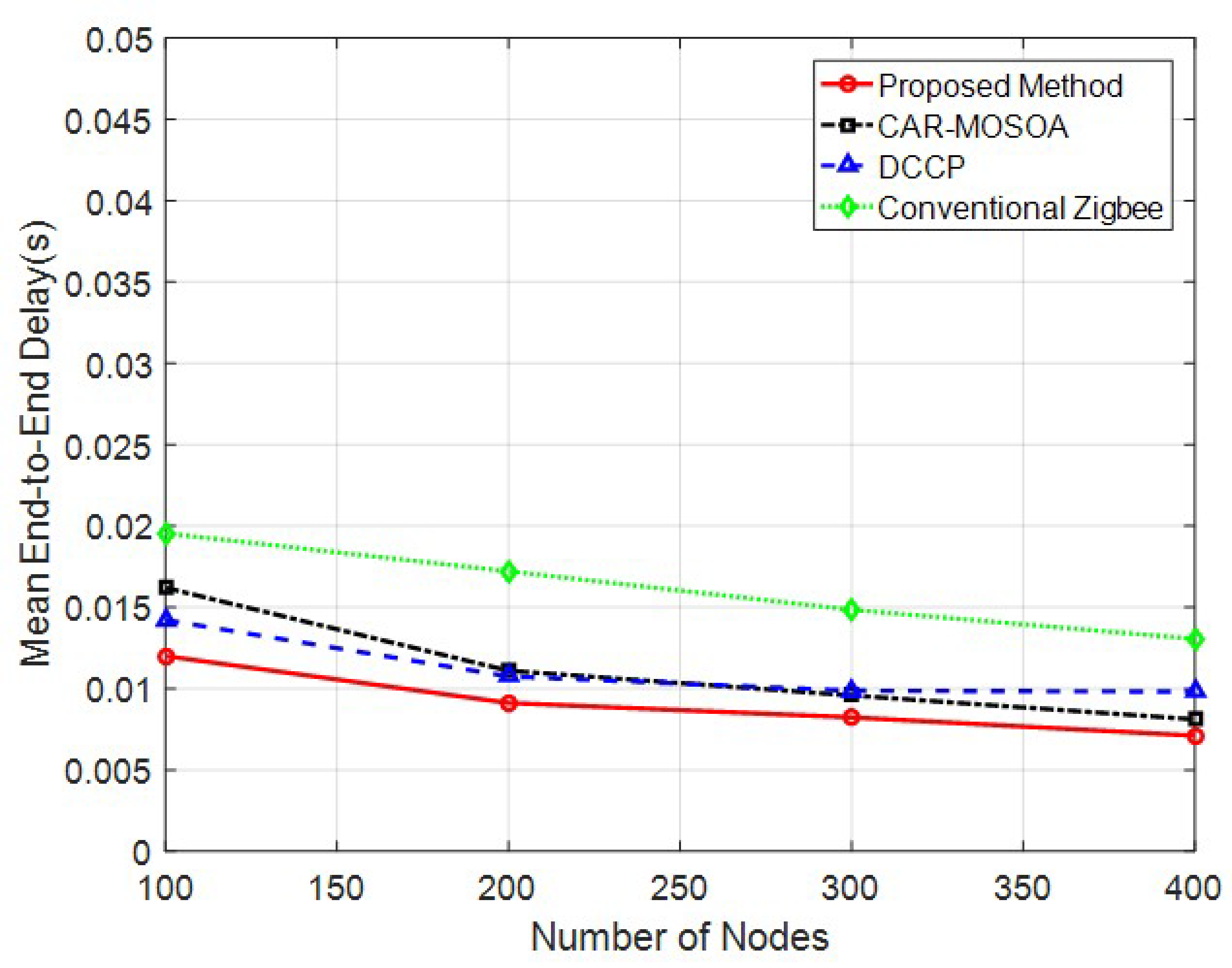
4.1. Change in the Number of Network Nodes

In this experiment, the effect of changes in the number of network nodes on the performance of CARLA was studied. In this test, the number of mobile nodes in the network was changed between 100 and 400 nodes, and the parameters of total energy consumption and PDR were calculated for different situations. Figure 8 shows the PDR graph for these changes.

As shown in Figure 8, with the increase in the number of network nodes, PDR also increases. The increase in the number of active nodes in the IoT network causes the number of routes between network nodes to increase. The result of this characteristic is the increase in the probability of optimal communication and, as a result, the formation of a more suitable topology for packet exchange in the network. As shown in the results of Figure 8, CARLA, by using the local hierarchical tree structure based on MBF, works more efficiently in forming the topology structure and performs the routing operation with a higher successful delivery ratio. Comparing the PDR values of the proposed method with the results obtained for the conventional Zigbee protocol demonstrates that the proposed routing strategy is effective in improving the probability of successful delivery of packets. On the other hand, CARLA outperforms the CAR-MOSOA and DCCP methods in terms of PDR, which can be attributed to the result of using the reinforcement learning ability of LAs in preventing congestion via the appropriate selection of the data rate for each node. In the proposed method, the adjustment of the data rate in each node is performed through monitoring the individual PDR of the node. This mechanism is effective in improving the overall PDR of the network, while in the DCCP method, congestion control is performed reactively and can contribute to increasing the possibility of packet loss. Figure 9 shows the graph of the total energy consumption for changes in the number of active nodes in the network.

Based on the results shown in Figure 9, increasing the number of network nodes will increase energy consumption because with the increase in the number of active nodes, the number of packets exchanged in the network also increases. Sending and receiving these packets requires energy consumption, and as a result of this feature, the energy consumption of the entire network will increase. Using a local hierarchical tree topology based on MBF in CARLA causes the data packets to be sent to the destination in fewer steps. On the other hand, the proposed topology structure requires fewer control packet exchanges for construction in each cycle, which results in less energy consumption. Furthermore, as shown in Figure 8, the probability of packet loss in CARLA is lower than in the compared method, which means fewer attempts for resending packets. For this reason, the energy consumption of CARLA is lower than the compared method. Figure 10 shows the graph of the average end-to-end delay in routing for changes in the number of network nodes.

When the number of network nodes increases, the number of routes between network nodes also increases. This condition causes the routing algorithm to have more choices for the route of sending data in the network. Therefore, increasing the number of nodes distributes the network’s traffic load among more nodes. As a result, the network’s traffic load will be evenly distributed on the network level, and the possibility of congestion will be reduced. For this reason, the end-to-end delay graph in Figure 10 is descending. As described in the Section 3, the level of buffer occupancy is one of the parameters used in CARLA to determine the weight of topology connections. This feature causes CARLA to have a lower end-to-end delay in the data routing process for different numbers of nodes because CARLA will be more inclined to choose routes with less delay. On the other hand, route discovery and selection in methods such as CAR-MOSOA and DCCP is time consuming, which results in increasing the end-to-end delay. As a result, as shown in this figure, the end-to-end delay, on average, is less than in the compared methods.

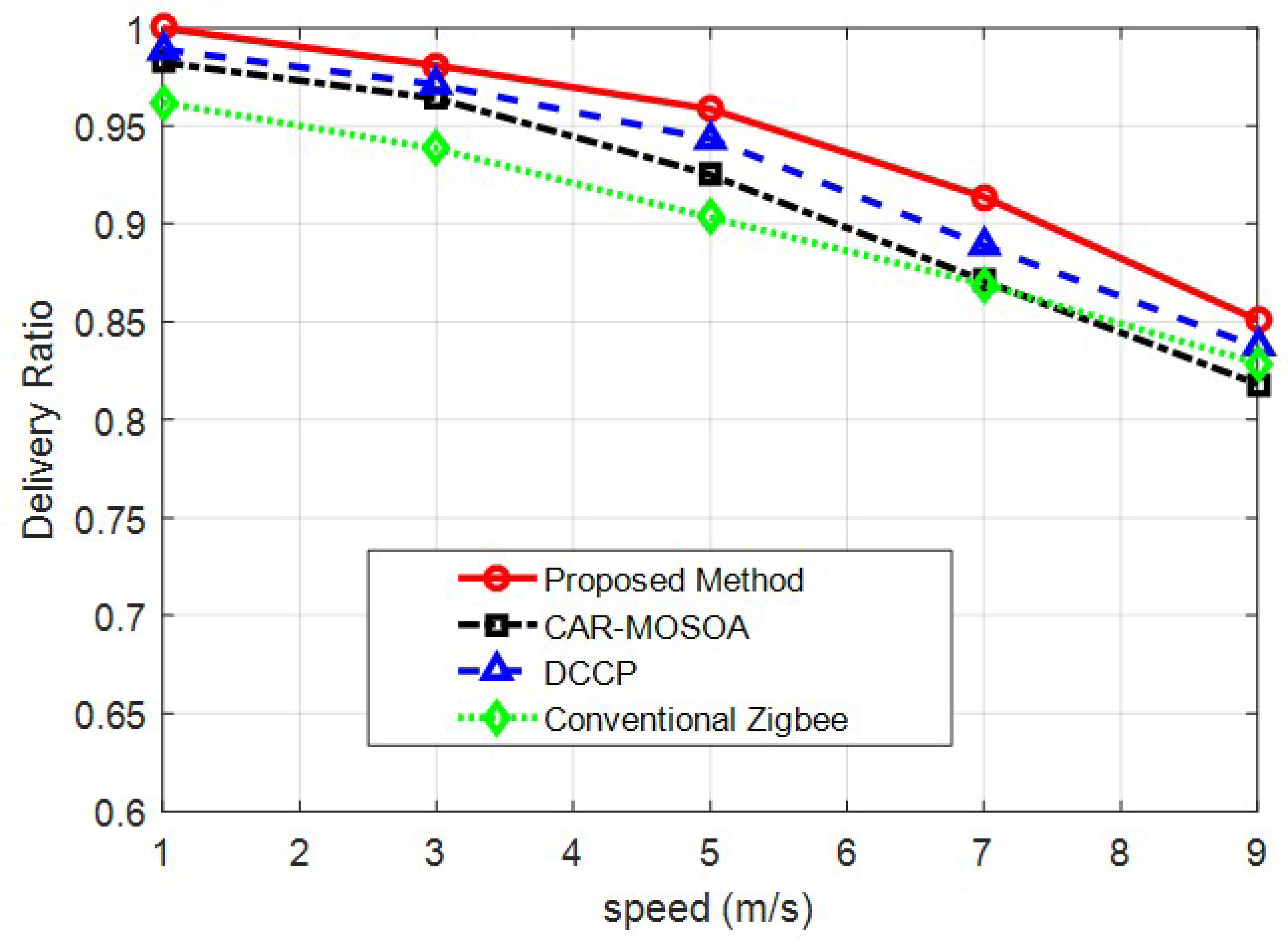
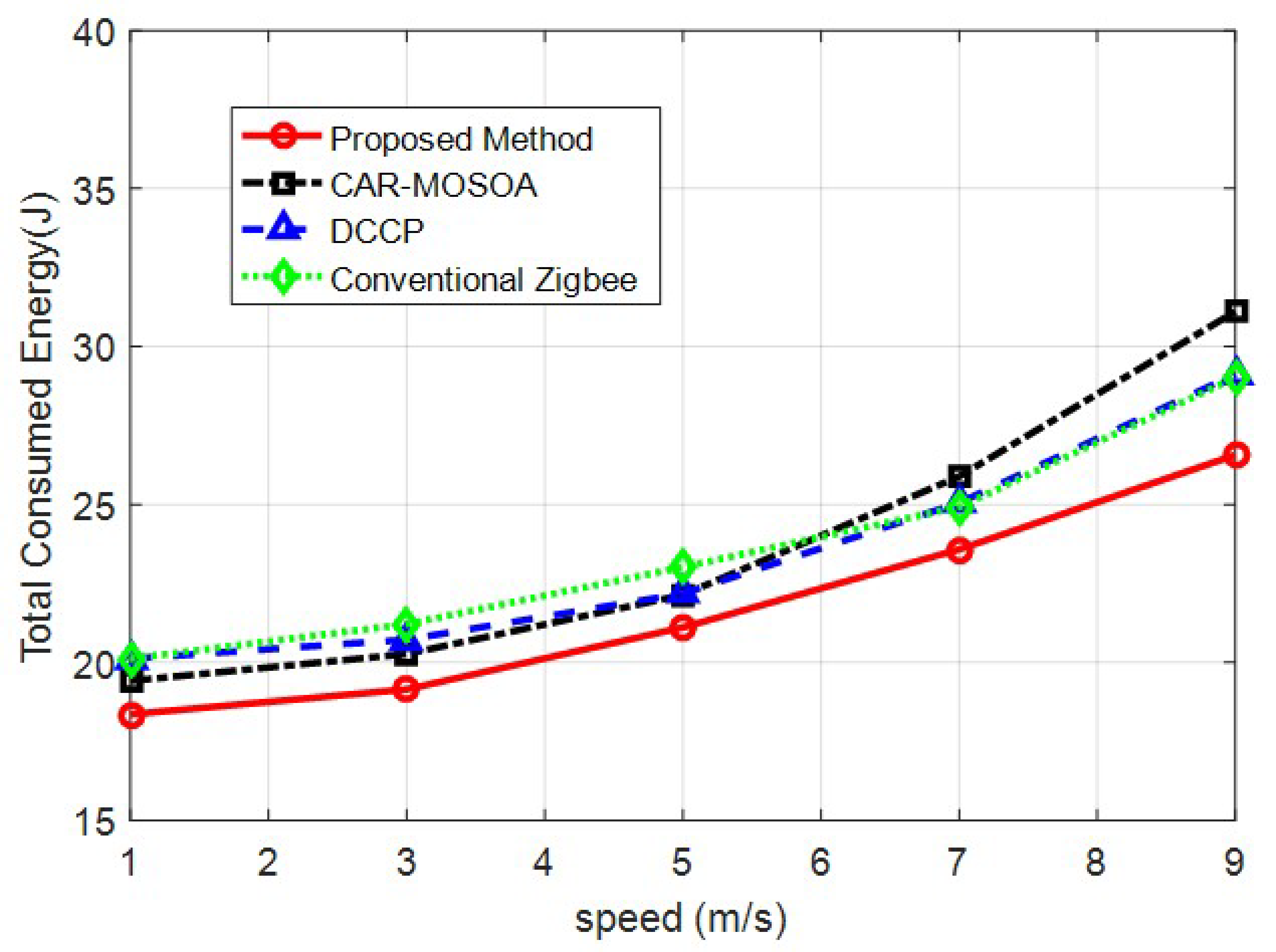
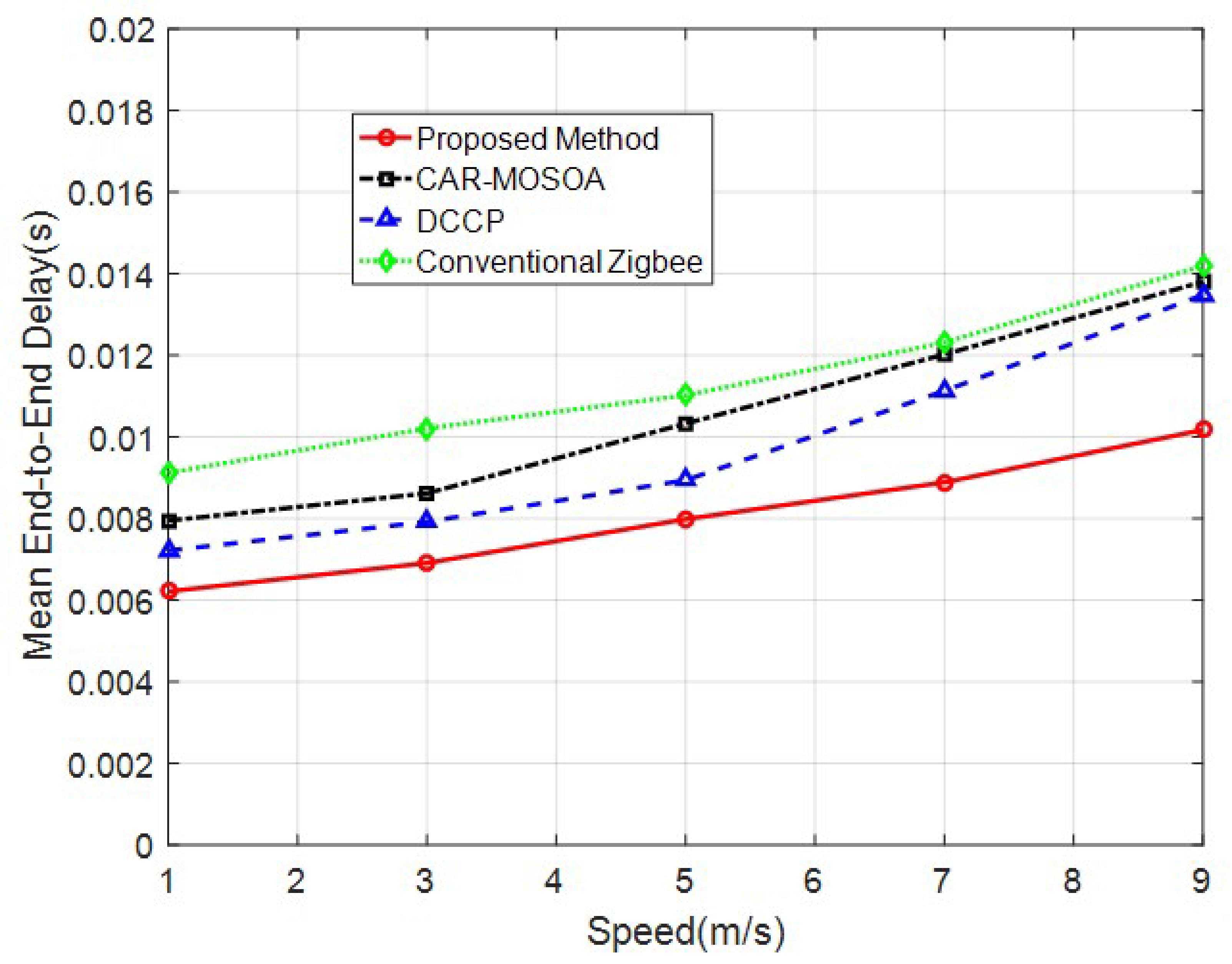
4.2. Changes in the Speed of Mobile Nodes

In this experiment, the effect of changes in the mobility speed of network nodes on the performance of CARLA was investigated. In this test, the number of nodes in the network is set to 100, and the speed of the nodes is changed in the range of 1 to 9 m per second. For these changes, the parameters of PDR, energy consumption, and end-to-end delay were calculated for different situations. In Figure 11, the graph of the PDR for the different speeds of network nodes is displayed.

Based on Figure 11, CARLA can successfully deliver the packets exchanged in the network to the destination with a higher probability. Increasing the speed of network nodes causes the lifetime of communication between network nodes to decrease because with the increase in speed, each node can travel a greater distance per second, and as a result, the probability of nodes moving out of each other’s neighborhood range increases. In CARLA, the rate of successful packet routing by nodes is considered one of the route selection criteria. This criterion makes the topology structure formed in CARLA consider connections for routing packets in the network, which can perform packet routing with a higher probability of success, even in critical conditions. For this reason, the PDR in CARLA is higher than in the compared method. Figure 12 shows the total energy consumption graph for changes in the speed of network nodes.

Based on the results shown in Figure 12, increasing the speed of network nodes increases energy consumption. Increasing the speed of the nodes will reduce the lifespan of the topology, and as a result, the number of attempts to resend the packet will increase. This increase in the number of attempts increases the network energy consumption. For this reason, the energy consumption diagram for changes in the network nodes’ speed is ascending in Figure 12. In CARLA, data packets are generally routed to their destination through nodes with a higher energy and probability of success. This feature causes the energy consumption of CARLA to decrease compared to other methods. Figure 13 shows the graph of the average end-to-end delay in routing for changes in the speed of network nodes.

According to the results of this experiment, the end-to-end delay also increases with the speed of the nodes. Due to increased speed conditions, the network nodes remain in the neighborhood for a shorter period, and the topology update operation is performed in shorter intervals. In this situation, the number of each node’s attempts to resend data increases, and as a result, the delay increases due to the increase in the waiting time of intermediate nodes. However, as mentioned, CARLA, considering the delay criterion as one of the route selection factors, causes the routes to be selected for data transmission with less delay. For this reason, the average end-to-end delay of CARLA in this experiment is lower than in the compared method. The MBF-based routing strategy in CARLA is effective in its efficiency and flexibility. In this structure, by determining the amount of memory allocated to each BF, the approximate amount of filter error in the search operation can be determined. Hence, it can be concluded that the structure presented in CARLA has no problem with the memory limitation of network nodes. It can be used in any size of memory and with any number of nodes in the network. Adjustable speed and accuracy in searching are other advantages of using the proposed MBF structure. By determining the number of bits of each BF in the MBF structure presented, the speed of searching the route and the accuracy of the search result can be determined. These parameters increase with the increase in the number of allocated bits. For example, in a network with 100 nodes, if we consider the number of bits required for each BF equal to 100 bits, the MBF will be able to detect the existence of the route with 100% accuracy with just one comparison. The maximum space required for the MBF in this example is 1.22 KB.

The numerical results of the experiments are summarized in

Table 2. Numerical results of the experiments.

Experiment	Method	PDR	Energy (j)	Delay (s)
Number of Nodes	Proposed Method	0.9425	28.39	0.009116
	CAR-MOSOA [15]	0.8691	34.48	0.01125
	DCCP [16]	0.9064	31.12	0.01116
	Conventional Zigbee	0.8684	34.86	0.01616
Speed of Nodes	Proposed Method	0.9408	21.75	0.008035
	CAR-MOSOA [15]	0.9121	23.76	0.01055
	DCCP [16]	0.9259	23.42	0.009738
	Conventional Zigbee	0.9003	23.66	0.01137

. As the results in this table demonstrate, CARLA can outperform the compared methods in terms of the average PDR, average energy consumption, and average end-to-end delay. According to the results, CARLA improves the average PDR by 5.7% compared to the conventional Zigbee protocol. Moreover, at least an 8.07% and 29.33% reduction in the energy consumption and end-to-end delay could be achieved by using CARLA, compared to the conventional Zigbee protocol. Comparing the results obtained by the proposed method with previous efforts shows that CARLA can improve PDR by 4.64%, and at the same time, reduce the energy consumption and end-to-end delay by 11.44% and 25.26%, respectively. These results confirm the effectiveness of CARLA in improving the network performance in different conditions.

In order to more closely examine the performance of CARLA in avoiding congestion, it is necessary to investigate its mechanism for determining the data rate of network nodes with LA. For this purpose, the data rate values and the buffer memory occupancy level of the active nodes of the network are checked according to their position in the environment. The base station location can cause an overall change in the network traffic patterns [25]. In this case, a network with dimensions of 100 m × 100 m, with 100 sensor nodes in different conditions of the base station placement, is considered. Figure 14 displays the results for the case where the base station is located in the center of the environment (50,50). Figure 14a shows the data rate determined for each node according to their position in one of the simulation periods. Further, Figure 14b shows the occupied buffer rates of the nodes at this point.

Based on Figure 14a, the LA used in CARLA determines the data rate of the network nodes independently and according to the conditions of the nodes. By examining this figure, it can be seen that the nodes located in the center of the environment (the nodes adjacent to the base station) have a higher data rate than the peripheral nodes of the network. The reason for this can be attributed to the increased traffic of the central nodes of the network because, in this case, the nodes adjacent to the base station, in addition to their own data, must also participate in forwarding the data of distant nodes. As a result, these nodes will need to send data packets at a higher rate to prevent congestion in the network. On the other hand, Figure 14b shows that increasing the data rate of the central nodes can primarily avoid the increase of the occupied buffer rate of these nodes. These results indicate that in all the nodes, the occupied buffer rate of the nodes is less than 0.8, which, according to the acceptable PDR in CARLA, shows its efficiency in avoiding memory overflow and congestion. These results confirm that the LA used in the nodes can determine the optimal data rate for each node in such a way that it can keep PDR high, while avoiding congestion and the formation of communication bottlenecks in high-traffic areas of the network (around the base station). In Figure 15, similar results for the same nodes in the condition that the base station is located in the corner of the environment are shown.

Examining the graphs presented in this figure confirms the claims made based on Figure 14. By comparing Figure 14a and Figure 15a, it can be seen that the data rate determined for things is related to their topological position. However, it should be noted that LA does not determine the data rate values of the sensor nodes based on their position relative to the base station, but rather, this action is performed based on the load imposed on the nodes and to maximize their successful delivery ratio. On the other hand, comparing the graphs of nodes’ occupied buffer rates based on their position in Figure 14b and Figure 15b shows that CARLA can, independently of the topological position, overflow the nodes’ buffer and prevent congestion in the network. These diagrams show that the occupied buffer rate of each node is independent of its position (and the traffic load imposed on it). The reason for this is the deployment of LA in each node independently, based on which the optimal sending rate is determined for each node individually and based on its conditions. These results show that CARLA prevents congestion, especially in areas with high data traffic.

5. Conclusions

This article presented a new solution, named CARLA, to avoid congestion in intelligent transport networks based on WSN-IoT infrastructure. CARLA is based on two efficient tools: MBF and LA. In this method, the Bloom structure of multiple filters was used to form a topology and manage the communication structure of things locally. Using this structure has several advantages. Forming the proposed topology structure imposes minimum overhead on the network. On the other hand, the structure based on the proposed MBF provides the possibility of fast communication updates according to the dynamic conditions of the network. In CARLA, LA is also used to determine the optimal data rate of distributed things. The use of a reward and penalty strategy in this learning model makes the LA located in each node able to determine the optimal strategy for determining the data rate based on the specific conditions of that node. The efficiency of CARLA was compared with the conventional Zigbee protocol and recent works. Compared to the conventional Zigbee protocol, CARLA improves the average PDR by 5.7% and reduces energy consumption and the end-to-end delay by at least 8.07% and 29.33%, respectively. In addition, compared to the CAR-MSOA and DCCP methods, CARLA can improve PDR by 4.64% and reduce energy consumption and the end-to-end delay by 11.44% and 25.26%, respectively.

One of the limitations of CARLA in this research is not considering the priority of the data exchanged in the network. In future works, the proposed solution will be improved to solve this limitation. For this purpose, it is possible to determine the number of bits assigned to the MBF by considering the data priority of each node. Another limitation of this research is the practical implementation of CARLA, which needs relatively large modifications of the topology control and routing modules of the Zigbee protocol. This case will also be considered one of the future research goals, along with improving the performance of CARLA.

References

1. Fahmy, H.M.A. Wireless Sensor Networks; Springer International Publishing: Berlin/Heidelberg, Germany, 2020. [Google Scholar]
2. Jain, V.K.; Mazumdar, A.P.; Faruki, P.; Govil, M.C. Congestion control in Internet of Things: Classification, challenges, and future directions. Sustain. Comput. Inform. Syst. 2022, 35, 100678. [Google Scholar] [CrossRef]
3. Yadav, S.L.; Ujjwal, R.L. Mitigating congestion in wireless sensor networks through clustering and queue assistance: A survey. J. Intell. Manuf. 2021, 32, 2083–2098. [Google Scholar] [CrossRef]
4. Cao, K.; Ding, H.; Wang, B.; Lv, L.; Tian, J.; Wei, Q.; Gong, F. Enhancing Physical Layer Security for IoT with Non-Orthogonal Multiple Access Assisted Semi-Grant-Free Transmission. IEEE Internet Things J. 2022, 9, 24669–24681. [Google Scholar] [CrossRef]
5. Dai, X.; Xiao, Z.; Jiang, H.; Alazab, M.; Lui, J.C.; Dustdar, S.; Liu, J. Task co-offloading for d2d-assisted mobile edge computing in industrial internet of things. IEEE Trans. Ind. Inform. 2022, 19, 480–490. [Google Scholar] [CrossRef]
6. Yuan, H.; Yang, B. System Dynamics Approach for Evaluating the Interconnection Performance of Cross-Border Transport Infrastructure. J. Manag. Eng. 2022, 38, 04022008. [Google Scholar] [CrossRef]
7. Balador, A.; Cinque, E.; Pratesi, M.; Valentini, F.; Bai, C.; Gómez, A.A.; Mohammadi, M. Survey on decentralized congestion control methods for vehicular communication. Veh. Commun. 2021, 33, 100394. [Google Scholar] [CrossRef]
8. Godoy, P.D.; Cayssials, R.L.; Garino, C.G.G. Communication channel occupation and congestion in wireless sensor networks. Comput. Electr. Eng. 2018, 72, 846–858. [Google Scholar] [CrossRef]
9. Bohloulzadeh, A.; Rajaei, M. A survey on congestion control protocols in wireless sensor networks. Int. J. Wirel. Inf. Netw. 2020, 27, 365–384. [Google Scholar] [CrossRef]
10. Grover, A.; Kumar, R.M.; Angurala, M.; Singh, M.; Sheetal, A.; Maheswar, R. Rate aware congestion control mechanism for wireless sensor networks. Alex. Eng. J. 2022, 61, 4765–4777. [Google Scholar] [CrossRef]
11. Gherbi, C.; Roumaissa, D. IoT based traffic congestion control for environmental applications. Informatica 2021, 45, 13–23. [Google Scholar] [CrossRef]
12. Upreti, K.; Kumar, N.; Alam, M.S.; Verma, A.; Nandan, M.; Gupta, A.K. Machine learning-based Congestion Control Routing strategy for healthcare IoT enabled wireless sensor networks. In Proceedings of the 2021 Fourth International Conference on Electrical, Computer and Communication Technologies (ICECCT), Erode, India, 15–17 September 2021; pp. 1–6. [Google Scholar]
13. Sankari, B.S.; Nemani, R. Squirrel Search Algorithm Based Support Vector Machine for Congestion Control in WSN-IoT. Wirel. Pers. Commun. 2022, 124, 1945–1960. [Google Scholar] [CrossRef]
14. Kasthuribai, P.T. Optimized support vector machine-based congestion control in wireless sensor network-based Internet of Things. Int. J. Comput. Netw. Appl. 2021, 8, 444–454. [Google Scholar] [CrossRef]
15. Jagannathan, P.; Gurumoorthy, S.; Stateczny, A.; Divakarachar, P.B.; Sengupta, J. Collision-Aware Routing Using Multi-Objective Seagull Optimization Algorithm for WSN-Based IoT. Sensors 2021, 21, 8496. [Google Scholar] [CrossRef] [PubMed]
16. Majeed, U.; Malik, A.N.; Abbas, N.; Abbass, W. An Energy-Efficient Distributed Congestion Control Protocol for Wireless Multimedia Sensor Networks. Electronics 2022, 11, 3265. [Google Scholar] [CrossRef]
17. Kaur, G.; Chanak, P.; Bhattacharya, M. A Green Hybrid Congestion Management Scheme for IoT-enabled WSNs. IEEE Trans. Green Commun. Netw. 2022, 6, 2144–2155. [Google Scholar] [CrossRef]
18. Suma, S.; Harsoor, B. Dynamic shortest path routing algorithm to reduce retransmission and congestion avoidance for mobile nodes in wireless sensor network. In IoT Based Control Networks and Intelligent Systems; Springer: Berlin/Heidelberg, Germany, 2022; pp. 649–659. [Google Scholar]
19. Chappala, R.; Anuradha, C.; Murthy, P.S.R.C. Adaptive Congestion Window Algorithm for the Internet of Things Enabled Networks. Int. J. Adv. Comput. Sci. Appl. 2021, 12. [Google Scholar] [CrossRef]
20. Srivastava, V.; Tripathi, S.; Singh, K.; Son, L.H. Energy efficient optimized rate-based congestion control routing in wireless sensor network. J. Ambient. Intell. Humaniz. Comput. 2020, 11, 1325–1338. [Google Scholar] [CrossRef]
21. Alejandrino, J.; Concepcion, R.; Lauguico, S.; Palconit, M.G.; Bandala, A.; Dadios, E. Congestion detection in wireless sensor networks based on artificial neural network and support vector machine. In Proceedings of the 2020 IEEE 12th International Conference on Humanoid, Nanotechnology, Information Technology, Communication and Control, Environment, and Management (HNICEM), Manila, Philippines, 3–7 December 2020; pp. 1–6. [Google Scholar]
22. Khorov, E.; Kiryanov, A.; Lyakhov, A.; Bianchi, G. A tutorial on IEEE 802.11 ax high efficiency WLANs. IEEE Commun. Surv. Tutor. 2018, 21, 197–216. [Google Scholar] [CrossRef]
23. Patgiri, R.; Nayak, S.; Borgohain, S.K. rDBF: A r-dimensional bloom filter for massive scale membership query. J. Netw. Comput. Appl. 2019, 136, 100–113. [Google Scholar] [CrossRef]
24. Narendra, K.S.; Thathachar, M.A. Learning Automata: An Introduction; Courier Corporation: North Chelmsford, MA, USA, 2012. [Google Scholar]
25. Jiang, S.; Zhao, C.; Zhu, Y.; Wang, C.; Du, Y. A Practical and Economical Ultra-wideband Base Station Placement Approach for Indoor Autonomous Driving Systems. J. Adv. Transp. 2022, 2022, 3815306. [Google Scholar] [CrossRef]
Figure 1. Topology formation packet structure.
Electronics 12 02070 g001
Figure 2. Routing Data section in the topology formation step.
Electronics 12 02070 g002
Figure 3. Discovering the possible routes between different nodes and forming a topology tree structure related to it: (a) received control packets by node S6 during topology construction, (b) local hierarchical structure of node S6 according to the discovered routes.
Electronics 12 02070 g003
Figure 4. An example of MBF-based topology construction, (a) the local hierarchical structure formed by node S6, (b) the corresponding MBF structure after applying hash function.
Electronics 12 02070 g004
Figure 5. (a,b) Structure of the MBF before and after energy depletion of the S4 node with hash code 10001.
Electronics 12 02070 g005
Figure 6. Structure of LA and its interaction with the environment.
Electronics 12 02070 g006
Figure 7. Flowchart of route search using proposed method.
Electronics 12 02070 g007
Figure 8. PDR graph for different number of network nodes.
Electronics 12 02070 g008
Figure 9. Total energy consumption graph for different number of network nodes.
Electronics 12 02070 g009
Figure 10. Average end-to-end delay for different number of network nodes.
Electronics 12 02070 g010
Figure 11. PDR graph for different speeds of network nodes.
Electronics 12 02070 g011
Figure 12. Total energy consumption graph for different speeds of network nodes.
Electronics 12 02070 g012
Figure 13. Average end-to-end delay for different speeds of network nodes.
Electronics 12 02070 g013
Figure 14. (a) Data rate determined for each node according to its position and (b) the occupied buffer rate values of the nodes in a network with 100 nodes and the base station in the center of the environment.
Electronics 12 02070 g014
Figure 15. (a) Data rate determined for each node according to its position and (b) the occupied buffer rate values of the nodes in a network with 100 nodes and the base station in the corner of the environment.
Electronics 12 02070 g015