Discriminating WirelessHART Communication Devices Using Sub-Nyquist Stimulated Responses

Abstract

Reliable detection of counterfeit electronic, electrical, and electromechanical devices within critical information and communications technology systems ensures that operational integrity and resiliency are maintained. Counterfeit detection extends the device’s service life that spans manufacture and pre-installation to removal and disposition activity. This is addressed here using Distinct Native Attribute (DNA) fingerprinting while considering the effects of sub-Nyquist sampling on DNA-based discrimination. The sub-Nyquist sampled signals were obtained using factor-of-205 decimation on Nyquist-compliant WirelessHART response signals. The DNA is extracted from actively stimulated responses of eight commercial WirelessHART adapters and metrics introduced to characterize classifier performance. Adverse effects of sub-Nyquist decimation on active DNA fingerprinting are first demonstrated using a Multiple Discriminant Analysis (MDA) classifier. Relative to Nyquist feature performance, MDA sub-Nyquist performance included decreases in classification of %C_Δ ≈ 35.2% and counterfeit detection of %CDR_Δ ≈ 36.9% at SNR = −9 dB. Benefits of Convolutional Neural Network (CNN) processing are demonstrated and include a majority of this degradation being recovered. This includes an increase of %C_Δ ≈ 26.2% at SNR = −9 dB and average CNN counterfeit detection, precision, and recall rates all exceeding 90%.

1. Introduction

The development of new electronic, electrical, and electromechanical device technologies supporting critical information and communications technology systems will continue for decades to come. The deployment and availability of new devices provides certain benefits for expanding interconnectivity capabilities within the critical information and information technology arena. This expansion has heightened awareness and increased concerns associated with maintaining operational integrity and resiliency within the information and communications technology supply chain [1,2]. The adverse effects caused by a loss of operational integrity or resiliency range from increased inconvenience (degraded, inefficient, or intermittent service) at one extreme to premature lifecycle termination (removal from service) at the other extreme.

Supply chain integrity concerns are not unique within the information and communications technology community and are shared among other service communities that rely on electronic communications. Activities within these other service communities vary widely but are generally embodied within critical infrastructure, internet of things, industrial internet of things, and/or fourth industrial revolution frameworks [3,4,5,6]. Regardless of the framework, the use of digital communications requires that integrity assurance measures be taken during all phases of the device’s technical lifespan (service life) [5]. The demonstration emphasis here is on pre-deployment protection (i.e., counterfeit detection) applied within the near-cradle phase of the device’s technical lifespan. This includes pre-deployment manufacturing and distribution protection.

Lifespan assurance is addressed here using Radio Frequency (RF)-based Distinct Native Attribute (DNA) fingerprinting to provide reliable pre-deployment detection of counterfeit devices. Such protection can be considered during manufacturing, following manufacturing, and/or at any point in the supply chain as the device makes its way into service. A form of active DNA fingerprinting is considered here that uses fingerprint features extracted from externally stimulated responses of non-operating, non-operably connected WirelessHART communication devices. The operational and technical motivations for making this choice are presented in Section 1.1 and Section 1.2, respectively.

1.1. Operational Motivation

The operational motivation for considering Wireless Highway Addressable Remote Transducer (WirelessHART) field device discriminability is generally unchanged from that put forth in prior related works [5,7,8,9,10]. It is even reasonable to argue that the motivation today remains stronger than ever given that (1) the number of fielded WirelessHART devices has reached into the tens-of-millions [11], and (2) hundreds of thousands of WirelessHART devices are manufactured annually and enter the supply chain [12]. Since its initial introduction WirelessHART has been well-received in European and North American industries given that [3,9,11,12]:

• It operates using the legacy wired HART protocol and users can take maximum advantage of prior experience, training, tool purchases, etc.;
• The deployment, installation, and maintenance cost are considerably reduced since no additional infrastructure cabling is generally required;
• There is considerable network architecture flexibility and expansion is easily accommodated using additional field devices or by connecting other nearby networks;
• The time required to commission (bring into service and put online) new devices takes hours versus days thanks to efficient pre-deployment benchtop programing.

It has been noted that a five-device WirelessHART network provides “sufficiently redundant operation” [12] and flexibility to support general industrial network architectures [11] and the communications lifeline between critical infrastructure elements [13]. Thus, the consideration and demonstration of counterfeit detection using N_Dev = 8 hardware devices here is not overly simplified and has appropriate applicability to small-scale networks supporting information and communications technology applications.

The concerns with maintaining operational integrity and resiliency in critical information and communications technology systems [1,2] are not new and related protection criteria was established early in November 2009 by the Society of Automobile Engineers under SAE-AS6462 guidelines [14]. This guidance targeted aerospace applications and was adopted by the US Defense Logistics Agency in May 2014 [15]—they subsequently reaffirmed SAE-AS6462 relevance in April 2020. To cope with an expanding supply chain attack space, the SAE-AS6462 guidelines were subsequently updated to the most recent AS-5553D revision in March 2022 [16]. The evolution to AS-5553D includes the recognition of expanded applicability to all organizations (beyond aerospace) that procure “parts and/or systems, subsystems, or assemblies, regardless of type, size, and product provided”. AS-5553D aptly notes that mitigation of adverse counterfeit effects is “risk-based” and steps taken to mitigate these effects “will vary depending on the criticality of the application, desired performance and reliability of the equipment/hardware”.

1.2. Technical Motivation

Identifying counterfeit devices early in their lifecycle is crucial to ensuring that operational integrity and resiliency are maintained. Near-cradle counterfeit detection activity within the technical cradle-to-grave protection strategy [5] has been considered using fundamentally different RF-based approaches for various electronic, electrical, and electromechanical devices. Representative active stimulation methods include:

• RF-based fingerprinting that uses interrogated responses of intentionally embedded onboard structures emplaced during manufacture [6,17,18]. These methods embedded structures at the integrated circuit level to impart unique RF fingerprint features when stimulated. The stimulated features are extracted and used to track and verify device identity as it traverses the supply chain (manufacturer, distributor, installer);
• DNA-based fingerprinting that exploits inherently present uniqueness resulting from device component, sub-assembly, and/or manufacturing process differences [9,19,20,21]. These methods exploit stimulated features that are distinct (unique from device-to-device), native (instilled during manufacture), and collectively embody device hardware/operating attributes (power consumption, mode, status, etc.).

The work in [8] was the first to consider the discrimination of four -Siemens AW210 [22] and four Pepperl + Fuchs Bullet [23] WirelessHART adapters using active DNA fingerprinting. These demonstrations were motivated by earlier passive DNA fingerprinting works in [5] that used the same adapters. Passive DNA fingerprints are generated from devices that are operably connected and perform their normal by-design communication function. Subsequent demonstrations in [9] used the same WirelessHART adapters with passive DNA fingerprinting processes from [5,7] and the active DNA fingerprinting process from [8].

The work in [9] provides the main motivation for demonstrations performed here with a goal of improving overall computational efficiency and enhancing the operational transition potential. Several options were considered in [9], including the application of conventional signal processing (down-conversion and filtering) and factor-of-5 decimation of the active DNA stimulated responses from [8]. This provided (1) an effective sample rate reduction from 1 Giga Samples per second (GSps) to 200 Mega Samples per second (MSps) and (2) a corresponding decrease in the number of pulse time domain samples (1,150,000 to 230,000) used for DNA fingerprint generation.

1.3. Relationship to Prior Research

Numerous RF fingerprinting methods have been considered as a means to discriminate electrical, electronic, and electromechanical components, and to improve operational reliability and security. For brevity, a detailed summary of RF fingerprinting methods is not included in this paper and the reader is referred to [24]. The authors in [24] have done a commendable job of categorizing various RF fingerprinting methods that use physical layer features to discriminate transmission sources. While the overall end-to-end identification process for the various methods can vary considerably, the main task of signal collection and digitization is largely the same and aimed at capturing signals that contain “useful features” to enable reliable identification. What is not immediately evident in [24] and the various fingerprinting works noted therein, is the Nyquist sampling conditions and how satisfying them does or does not impact the ability to extract useful features. This is not saying that these prior works did not consider Nyquist conditions, but rather that details for this consideration are not explicitly detailed in the works.

A majority of the works in [24] are believed to be based on discriminating features extracted from Nyquist sampled signal responses. This is a consequence of the researchers (1) considering conventional digital signal processing techniques that include consideration for Nyquist sampling conditions, or (2) using collected signals and/or methods from related work(s) where Nyquist sampling criteria were maintained. Satisfying Nyquist criteria enables receiver systems to reliably reconstruct the transmitted signal of interest and perform their intended by-design function (communicate, navigate, track, etc.). Nyquist criteria include sampling the signal of interest at a rate equal to, or greater than, the maximum system operating frequency—as operating frequency increases so does the amount of sampled data and required computational resources. The desire to minimize the amount of sampled data has motivated extensive research over the past decade. These works demonstrate acceptable signal reconstruction using a reduced number of samples without satisfying Nyquist criteria [25,26,27,28]—these are but a few representative works from a search using sub-Nyquist, undersampling, and compressive sensing terms.

Given the lack of detailed discussion on Nyquist sampling conditions in the RF fingerprinting works noted in [24], the authors believe that the work presented here is perhaps the first to consider a direct comparison of fingerprint discrimination performance with (1) fingerprint features generated under both Nyquist and sub-Nyquist conditions, (2) using the same collected device responses, and (3) a given classifier architecture. While work remains to consider sub-Nyquist conditions for other signal types and fingerprinting methods, results here suggest that deviating from Nyquist sampling constraints is a viable option and fingerprinting can be performed without regard for preserving by-design signal information.

1.4. Paper Organization

The remainder of this paper is organized as follows. The Demonstration Methodology is presented in Section 2 which provides selected details for relevant processes used to generate the demonstration results. This includes details for Experimental Collection and Post-Collection Processing in Section 2.1, Nyquist Decimation in Section 2.2, Sub-Nyquist Decimation in Section 2.3, Time Domain DNA Fingerprint Generation in Section 2.4, and Multiple Discriminant Analysis (MDA) in Section 2.5. Section 2.5 includes two sub-sections that provide details for Device Classification in Section 2.5.1 and Device ID Verification in Section 2.5.2. Details for Convolutional Neural Network (CNN) Discrimination is provided in Section 2.6. This includes implementation details for the one-dimensional CNN (1D-CNN) architecture in Section 2.6.1 and the two-dimensional CNN (2D-CNN) architecture in Section 2.6.2. Section 3 provides the Device Discrimination Results and includes MDA Classification Performance in Section 3.1 and CNN Classification Performance in Section 3.2. The final Counterfeit Discrimination Assessment results are presented in Section 3.3 and the paper concludes with the Summary and Conclusions presented in Section 4.

2. Demonstration Methodology

This section summarizes the experimental demonstration steps used to generate the classification results presented in Section 3. These steps include:

• Experimental Collection and Post-Collection Processing in Section 2.1: this includes a summary of processing details from [8] for obtaining the post-collected WirelessHART s_PC(t) responses used here for Nyquist and sub-Nyquist decimation prior to DNA fingerprint generation. Selected details are provided for SFM waveform stimulus generation, WirelessHART device under test hardware, device under test response collection, and pre-fingerprint generation processing.
• Nyquist Decimation in Section 2.2: this includes the use of a theoretically selected NDecFac = 5 decimation factor based on conventional signal processing aimed at preserving by-design signal information. This process was first considered in [9] and was revisited here for completeness in making a Nyquist versus sub-Nyquist comparative performance assessment. In this case, decimation of s_PC(t) by the NDecFac = 5 factor was preceded by down-conversion (D/C) to near-baseband and BandPass (BP) filtering. The uniform frequency spacing of the SFM sub-pulses and overall SFM waveform bandwidth are maintained.
• Sub-Nyquist Decimation in Section 2.3: this includes the use of an empirically selected NDecFac = 205 decimation factor that is applied without regard for preserving by-design signal information. Empirical selection details are provided and include (1) consideration of community feedback received as part of [20] proceedings, and (2) the desire to maintain both the number of SFM tones present and their spectral domain relationship. The NDecFac = 205 factor provided the desired sample rate reduction and computational efficiency increase.
• Time Domain DNA Fingerprint Generation in Section 2.4: this includes selected details for the time domain DNA fingerprint generation process adopted from prior related work in [8,9]. The adopted process has steadily evolved through numerous demonstrations in wireless communications applying time domain DNA fingerprinting to multiple modulation types and having similar classification objectives.
• Multiple Discriminant Analysis (MDA) Discrimination in Section 2.5: this includes a description of MDA model development and MDA-based device classification (discrimination). The confusion matrix construction is presented and calculation of the average cross-class percent correct classification (%C) metric is defined.
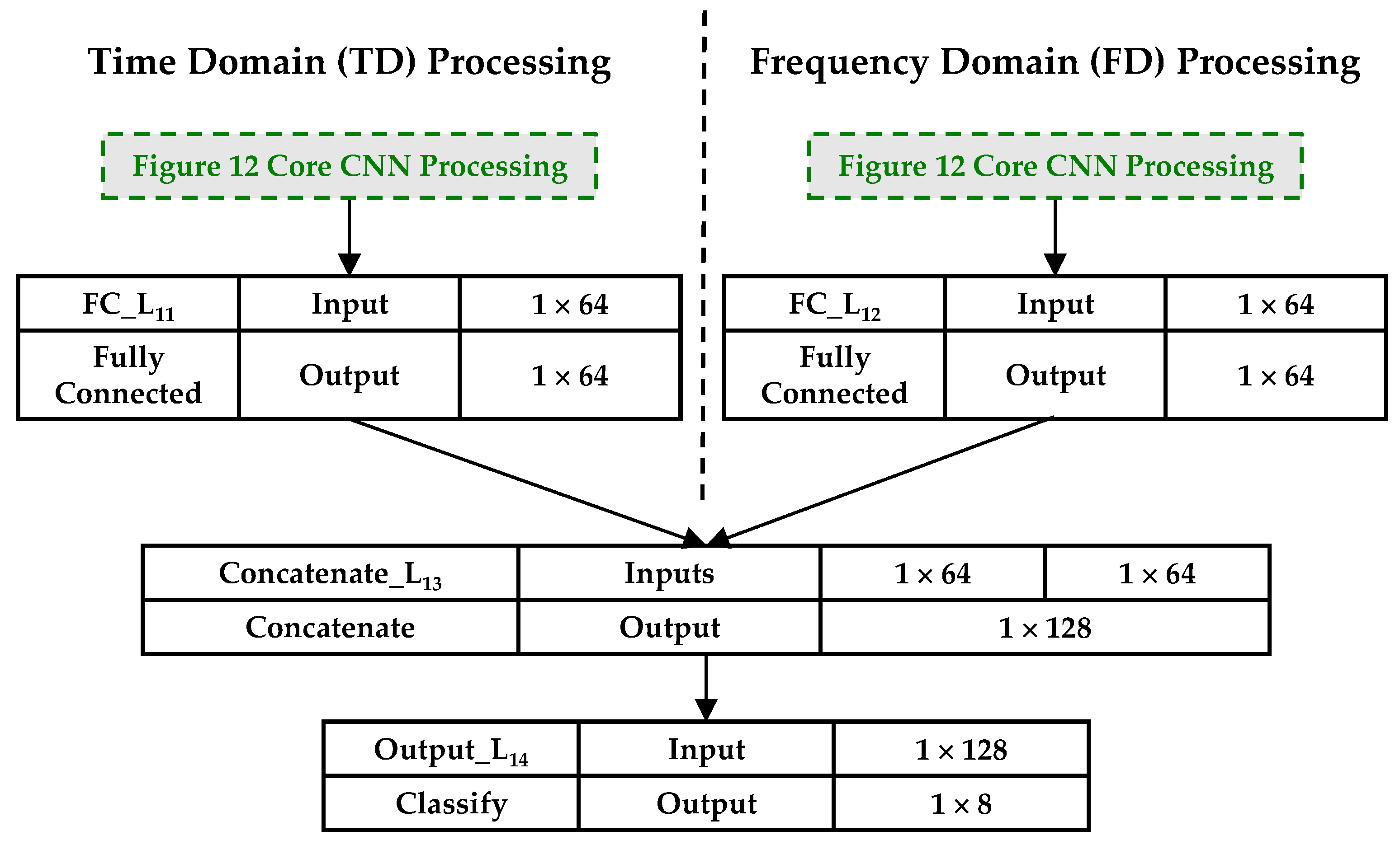
• Convolutional Neural Network (CNN) Discrimination in Section 2.6: this includes the CNN architectures selected for demonstration and the layer constructions used for performing (1) one-dimensional CNN (1D-CNN) processing with Time-Domain-Only (TDO) and Frequency-Domain-Only (FDO) samples, and (2) two-dimensional CNN (2D-CNN) processing with Joint-Time-Frequency (JTF) samples.

2.1. Experimental Collection and Post-Collection Processing

Stimulated WirelessHART response signals were originally collected and post-collection processed for demonstration activity in [8]. An overview of the collection setup is provided in Figure 1 and is based on integrated circuit anti-counterfeiting work in [18]. There are three main hardware components, including (1) a Keysight N5222B network analyzer [29] for generating the SFM input stimulus $s_{\mathrm{I}\mathrm{N}}\left(t\right)$, (2) a LeCroy WaveMaster 825Zi-A oscilloscope [30] for collecting the device under test output response $s_{\mathrm{O}\mathrm{U}\mathrm{T}}\left(t\right)$, and (3) the WirelessHART device under test.

Table 1. Selected details for N_Dev = 8 WirelessHART adapters used for demonstration.

Device ID	Device Label	Serial Number
D1	Siemens AW210	003095
D2	Siemens AW210	003159
D3	Siemens AW210	003097
D4	Siemens AW210	003150
D5	Pepperl + Fuchs Bullet	1A32DA
D6	Pepperl + Fuchs Bullet	1A32B3
D7	Pepperl + Fuchs Bullet	1A3226
D8	Pepperl + Fuchs Bullet	1A32A4

shows details for the four Siemens [22] and four Pepperl + Fuchs [23] WirelessHART adapters considered. The N_Dev = 8 adapters are identified as the D1, D2, …, and D8 devices for demonstration. Although the device labeling of Siemens AW210 and Pepperl + Fuchs Bullet devices makes it appear that they are from two different manufacturers, it was previously determined in [5] that these devices are actually from the same manufacturer. The devices were distributed under two different labels with dissimilar serial number sequencing (a result of company ownership transition). Thus, the device discrimination being considered is the most challenging, that is the like-model and intra-manufacturer case using identical hardware devices that vary only by serial number.

The N5222B source parameters were set to produce the SFM stimulus signal $s_{\mathrm{S}\mathrm{F}\mathrm{M}}\left(t\right)$ that was input as $s_{\mathrm{I}\mathrm{N}}\left(t\right)$ to 1-of-5 available adapter wires that are denoted as ${\mathrm{W}}_{\mathrm{I}\mathrm{N}}^j$ for j ∈ {1, 2, …, 5}. The SFM parameters were empirically set to maximize the source and device under test electromagnetic interaction with a goal of increasing discriminable information. The post-collected SFM response characteristics from [8] included (1) a total of N_SFM = 9 sub-pulses, (2) sub-pulse duration of T_Δ = 0.125 ms for a total SFM pulse duration of T_SFM = 1.125 ms, and (3) sub-pulse spectral spacing of f_Δ = 5 MHz yielding an SFM pulse bandwidth of W_SFM ≈ 50 MHz that approximately spans 400 MHz < f < 450 MHz. Each $s_{\mathrm{O}\mathrm{U}\mathrm{T}}\left(t\right)$ response received by the 825Zi-A oscilloscope was digitized, stored, and its corresponding output sample sequence {$s_{\mathrm{O}\mathrm{U}\mathrm{T}}\left(t\right)$} used for fingerprint generation.

As indicated in Figure 1, the SFM stimulus is applied to a given ${\mathrm{W}}_{\mathrm{I}\mathrm{N}}^j$ wire (j ∈ {1, 2, …, 5}) and the output response $s_{\mathrm{O}\mathrm{U}\mathrm{T}}\left(t\right)$ is collected from 1 of 4 remaining wires. The output collection wire is denoted as ${\mathrm{W}}_{\mathrm{O}\mathrm{U}\mathrm{T}}^k$ for k ∈ {1, 2, …, 5}, k ≠ j. Thus, there are a total of 20 order-matters ${\mathrm{W}}_{\mathrm{I}\mathrm{N}}^j:{\mathrm{W}}_{\mathrm{O}\mathrm{U}\mathrm{T}}^k$ permutations available for active DNA fingerprinting. The collections from [8] were used here for demonstration and included ${\mathrm{W}}_{\mathrm{I}\mathrm{N}}^j$ being the device input power wire and ${\mathrm{W}}_{\mathrm{O}\mathrm{U}\mathrm{T}}^k$ being the HART communication signaling wire.

2.2. Nyquist Decimation

Initial computational complexity reduction activity using the post-collected pulses from [8] was performed as part of work detailed in [9]. However, details of the theory-based Nyquist decimation process were omitted from [9] due to page constraints. Selected details are now included here to highlight differences between Nyquist decimated and the sub-Nyquist decimated processing detailed in Section 2.3. Processing of post-collected s_PC(t) pulses with Nyquist decimation is shown in Figure 2. The processing includes conventional signal processing of down-conversion (D/C), near-baseband BandPass (BP) filtering, decimation, and estimation of various powers and SNRs included.

The so-called “proper” decimation that is used here is consistent with Matlab’s downsample function and includes every NDecFac sample being retained and all others discarded. The desired effects of this decimation include (1) an effective sample rate reduction by a factor of 1/NDecFac (computational complexity reduction), and (2) retention of as-collected sample values and inherent source-to-device electromagnetic interaction effects (discriminable fingerprint information retention).

Figure 2 shows how the post-collected device response s_PC(t) is (1) Down-Converted (D/C) to near-baseband using a local oscillator frequency of f_LO = 375 MHz, (2) BandPass (BP) filtered at the D/C center frequency of f_D/C = 425 − 375 = 50 MHz using a 16th-order Butterworth filter having a passband of W_BP = 50 MHz, and (3) decimated by NDecFac = 5 to produce the decimated s_D(t)—this decimation factor choice was based on being the highest decimation factor that can be used while ensuring that Nyquist criteria is maintained. Thus, each of the WirelessHART s_PC(t) responses at a sample rate of f_S = 1 GSps (N_PC = 1,150,000 post-collected time domain samples per pulse) are converted to have an f_S = 200 MSps rate (N_Dec = 230,000 decimated time domain samples per pulse) prior to fingerprint generation. This processing was performed for all of the N_Pls = 1132 pulses that were collected and post-collection processed for each of the N_Dev = 8 WirelessHART adapters (D1, D2, …, D8) listed in Table 1.

The time domain effects of Figure 2 Nyquist decimation processing is illustrated for a representative WirelessHART s_PC(t) signal is in Figure 3. These plots are for the case where there is no like-filtered AWGN SNR scaling (SNR_A = SNR_PC). The Region of Interest (ROI) samples for DNA fingerprint generation are highlighted in Figure 3 as well. Apart from ROI sample index number changes required to ensure the pulse ROI duration remains unchanged following decimation, the time domain amplitude effects of sample decimation are minimally discernable.

The impact of Figure 2 Nyquist decimation processing is most evident in the frequency domain power spectral densities shown in Figure 4. This figure shows power spectral density (PSD) overlays for the (1) input s_PC(t) response (far right red), (2) down-converted s_D/C(t) response (far left green plus middle blue), and (3) final down-converted, bandpass filtered, and decimated s_D(t) response (far left green) used for the analysis s_A(t) generation. The impulse response (green dashed line) of the post-D/C bandpass filter W_BP is shown for reference. As desired for Figure 2 processing, the spectral content of s_D(t) is displaced but structurally unchanged from the input s_PC(t).

2.3. Sub-Nyquist Decimation

The main computational complexity reduction activity using post-collected WirelessHART pulses is referred to herein as sub-Nyquist decimation. Relative to the Nyquist decimation detailed in Section 2.2, the goal involves further reduction in the number of time domain samples in s_PC(t) used for classifier training and testing. The overall processing for sub-Nyquist decimation is illustrated in Figure 5. The indicated NDecFac = 205 decimation factor was empirically chosen and implemented through “proper” decimation. The choice of NDecFac = 205 was motivated by community feedback relative to the presentation made in support of [20]. This feedback included suggestions that “a minimum sample rate reduction of 200” should be considered to make the DNA fingerprinting method more attractive for adoption and operational implementation. The final choice of NDecFac = 205 was based on observing the decimated spectral responses and ensuring that both the number of SFM tones and the order of the tones were maintained. The process included “proper” decimation of s_PC(t) signals from [8] such that every 205th sample in the collections were retained and all others are discarded.

Nyquist sampling conditions of f_S = 1 GSps > 2 × f_Max = 2 × 425 MHz = 950 MHz were satisfied for the original post-collected s_PC(t) signals in [8]. Thus, application of the empirically chosen NDecFac = 205 proper decimation factor effectively yields sub-Nyquist sampled signals for DNA fingerprinting. As illustrated throughout the remainder of this subsection using the same representative SFM response pulse used for Section 2.2, the NDecFac = 205 sub-Nyquist decimation of s_PC(t) results in (1) the desired reduction in the number of samples used for fingerprint generation and classification, (2) an effective sample rate reduction by a factor of 1/NDecFac, and (3) inherent down-conversion, bandwidth compression, and increased background noise power in the spectral domain.

The sub-Nyquist decimation of SFM response signals was performed using an empirically chosen NDecFac = 205 decimation factor. The post-collection processing in [8] resulted in N_PC = 1,150,000 samples per SFM pulse at a sample frequency of f_S = 1 GSps. Thus, for the empirically chosen NDecFac = 205 factor, the sub-Nyquist decimated SFM pulses used here included a total of N_Dec = 1,150,000/205 = 5610 samples at a decimated sample rate of f_SDec = 1GSps/205 ≈ 4.88 MSps. The overall sub-Nyquist decimation process in Figure 5 was applied to a total of N_Pls = 1132 pulses that were collected and post-collection processed for each of the N_Dev = 8 WirelessHART devices being considered.

The effect of sub-Nyquist time domain sample decimation is illustrated in the amplitude responses shown in Figure 6. The ROI samples used for DNA fingerprint generation are highlighted as well. As implemented in [8], the post-collected SFM pulses are comprised of N_SFM = 9 sub-pulses, with (1) the duration of each sub-pulse being T_Δ = 0.125 ms and contributing to an overall SFM pulse duration of T_SFM = 9 × 0.125 ms ≈ 1.125 ms, and (2) the sub-pulses sequentially occurring at a uniform frequency spacing of f_Δ ≈ 5 MHz and contributing to an overall SFM pulse bandwidth of W_SFM ≈ 50 MHz. The T_SFM ≈ 1.125 ms pulse duration includes to a total of N_SPC = (1.125 ms × 1 GSps) ≈ 1,125,000 time domain samples in the post-collected pulse responses (Figure 6a) and N_SDec = (1.125 ms × 4.88 MSps) ≈ 5490 time domain samples in the decimated responses (Figure 6b) used for DNA fingerprinting.

The corresponding power spectral density (PSD) responses for sub-pulses contained in Figure 6 pulses are shown overlaid in Figure 7. The non-decimated SFM pulse bandwidth indicated in Figure 7a (dashed lines) is W_PC ≈ 50.0 MHz and spans a frequency range of 400 < f < 450 MHz. For the post-collected f_Max = 450 MHz and f_SPC = 1 GSps, the Nyquist criteria of f_SPC = 1 GSps ≥ 2 × 450 MSps = 900 MHz is satisfied for post-collection processed SFM pulses from [8]. The corresponding NDecFact = 205 decimated SFM pulse bandwidth in Figure 7b (dashed lines) is W_Dec ≈ 1.0 MHz and spans a frequency range of approximately 87 < f < 1150 KHz. For the decimated f_Max = 1150 KHz and the decimated f_SDec ≈ 4.88 MSps, the Nyquist criteria of f_SDec ≈ 4.88 MSps ≥ 2 × 1150 KHz ≈ 2.3 MHz is not satisfied for decimated SFM pulses and sub-Nyquist DNA fingerprinting is performed. Comparison of Figure 7a,b highlights the earlier noted down-conversion and bandwidth compression of s_PC(t) resulting from sub-Nyquist NDecFac = 205 decimation.

The power spectral densities for the composite SFM pulses are provided in Figure 8. Of note in comparing the non-decimated post-collected (PC) and decimated (Dec) responses in this figure are the average estimated background noise powers (N_PC and N_Dec) shown in the captions. The N_PC ≈ 5.54 × 10⁻⁵ (W/MHz) background noise power for Figure 8a was calculated as the average of seven noise powers estimated in seven adjacent ideal W_PC = 50.0 MHz filters (red dashed line regions) spanning 0 < f < 350 MHz. The decimated N_Dec ≈ 3.56 (W/MHz) background noise power for Figure 8b was calculated as the average noise power in a single ideal W_Dec ≈ 1.0 MHz filter (red dashed line region) spanning 13.5 < f < 23.5 MHz. Considering the ratio of N_D/N_PC noise powers, the difference in post-collected and sub-Nyquist decimated background noise powers (N_BΔ) is given by N_BΔ ≈ 10 × log10[3.56/(5.54 × 10⁻⁵)] ≈ 48.1 dB. This is the previously noted increased background noise power level resulting from sub-Nyquist decimation.

The overall pre-fingerprint generation processing with decimation, filtering, Signal-to-Noise Ratio (SNR) estimation and analysis SNR (SNR_A) scaling is illustrated in Figure 5. Using the post-collected SFM signal s_PC(t) and desired analysis SNR_A as inputs, the steps for generating analysis signal s_A(t) at the desired SNR_A include:

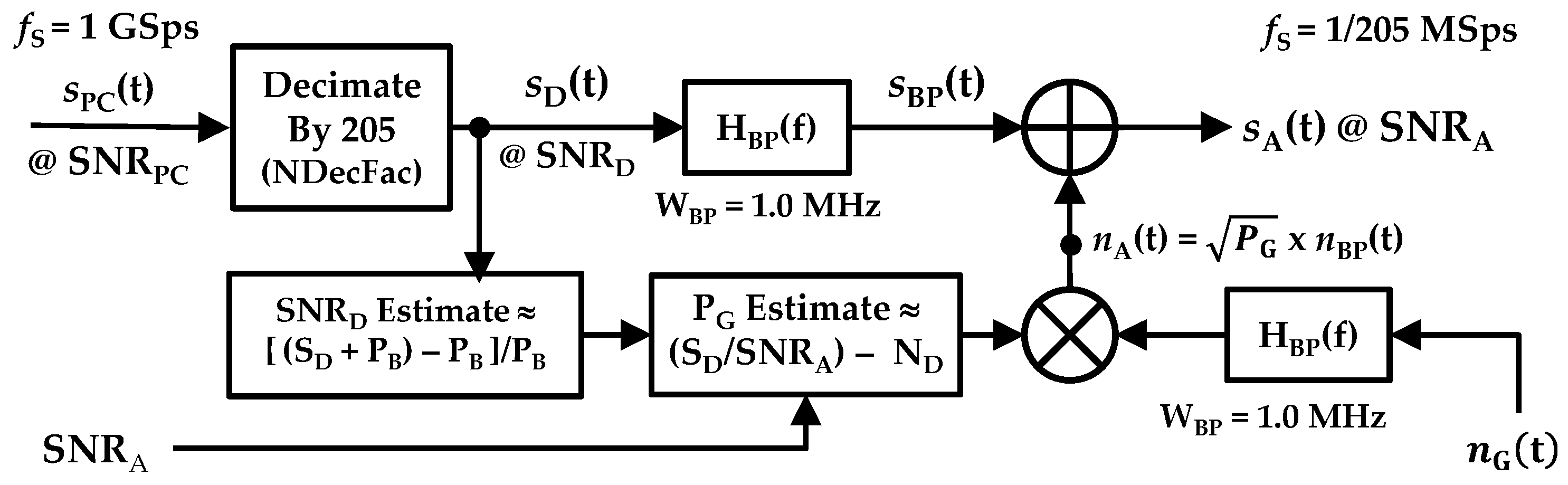
• Properly decimating s_PC(t) by the selected NDecFac factor to obtain s_D(t). The result is bandpass filtered with a W_Dec ≈ 1.0 MHz filter to produce s_BP(t).
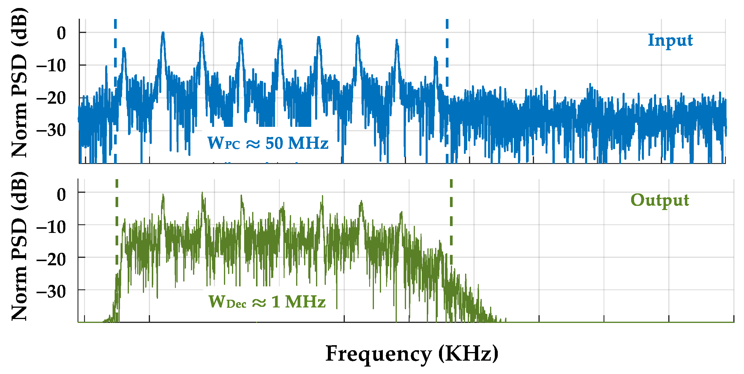
• Using s_D(t) to estimate the combined decimated signal and decimated noise (S_D + N_D) power using the signal-plus-background samples (see Figure 8b) that approximately span W_Dec ≈ 1.0 MHz.
• Estimating background noise power P_Dec using noise-only region samples (see Figure 8b) that approximately span W_Dec ≈ 1.0 MHz. The assumption here is that the estimated P_Dec noise power in this region is the same as the P_Dec noise power present in the estimated (S_Dec + P_Dec) power.
• Estimating s_D(t) signal-only power S_Dec using S_Dec ≈ (S_Dec + P_Dec) and the P_Dec noise power estimated in the previous step.
• Estimating the required like-filtered Additive White Gaussian Noise (AWGN) power as P_G ≈ (S_Dec/SNR_A). P_Dec using the desired SNR_A and the S_Dec and P_Dec power estimates from the two previous steps.
• Generating AWGN n_G(t) and BandPass (BP) filtering it with the W_Dec ≈ 1.0 MHz used to produce n_BP(t). The result is power-scaled by P_G to produce the noise analysis signal given by n_A(t) = $\sqrt{{\mathrm{P}}_{\mathrm{G}}}$ × n_BP(t).
• The final analysis signal s_A(t) at the desired SNR_A is formed as s_A(t) = s_BP(t) + n_A(t) and input to the DNA fingerprinting process.

The time and frequency domain effects of Figure 5 processing are shown in Figure 9 and Figure 10 for a NDecFac = 205 decimated s_D(t) SFM pulse at SNR_Dec ≈ 12.71 dB and a desired like-filtered power-scaled analysis s_A(t) at SNR_A = 0 dB. These plots were generated for the decimated s_D(t) of the representative SFM pulse used for Figure 8 responses. The estimated SNR_A ≈ 0 dB shown in Figure 9 and Figure 10 captions was estimated using the W_Dec ≈ 1.0 MHz decimation filter bandwidth. The final ROI samples used for time domain DNA fingerprint generation are highlighted in the bottom plot of Figure 9.

2.4. Time Domain DNA Fingerprint Generation

The time domain DNA generation process used here is a variant of previous passive [5,10,31,32] and more recent active [8,9] DNA-based fingerprinting works. Active DNA fingerprinting in [8,9] emerged from the earlier passive DNA fingerprinting methods [5,10,31,32] that steadily evolved within the wireless communications arena. Selected elements of time domain fingerprint generation are extracted from [9] and summarized here. The reader is referred to [9] and the other noted works for additional details.

The time domain region of interest samples from the analysis signals (those highlighted in Figure 9 and carried forward into Figure 11) are used to calculate statistical DNA features. For a real-valued sample sequence {s_FP(n)} the statistical DNA features are calculated for instantaneous (1) amplitude response samples given by M_FP(n) = |s_FP(n)|; (2) phase response samples given by Θ_FP(n) = tan⁻¹[H_Re(n)/ H_Im(n)] where H_Re(n) and H_Im(n) are real and imaginary components of the Hilbert Transform denoted by Hilbert[s_FP(n)]; and (3) frequency response samples given by Φ_FP(n) = gradient[Θ_FP(n)].

Statistical DNA features are calculated using the N_Resp = 3 instantaneous response sequences of {M_FP(n)}, {Θ_FP(n)}, and {Φ_FP(n)} and N_Srgn contiguous subregions of {s_FP(n)} that span the selected ROI. This is illustrated in Figure 11 which shows the {M(n)} magnitude responses for the representative pulse in Figure 9. Considering the calculation of N_Stat = 3 three statistical features of variance, skewness, and kurtosis [33] using samples within each of the N_Srgn = 18 subregions, and across the entire ROI as well, the time domain DNA fingerprints included a total of N_TD = (N_Srgn + 1) × N_Resp × N_Stat = (19 + 1) × 3 × 3 = 171 features.

2.5. Multiple Discriminant Analysis (MDA) Discrimination

The MDA-based discrimination methodology used here was adopted from prior related work in [5,8,9]. These works exploited DNA features for device discrimination using the same N_Dev = 8 WirelessHART adapters listed in Table 1 and used here. While providing a motivational basis for active DNA fingerprinting demonstration here, care is taken in making direct comparison of results in [5,8,9] with results provided here—this is reiterated with greater detail in Section 3 results. Regardless, the MDA processing here is fundamentally the same and summary details are presented for completeness. The reader is referred to [5] for additional details and a more complete development of MDA-based device classification.

MDA-based classification (discrimination) assessments were performed using a trained ($\mathbf{W}$, μ_F, σ_F, μ_n, Σ_n) MDA model—bold variables are used here and henceforth throughout the paper to denote non-scalar vector or matrix quantities. The model components include (1) the MDA projection matrix W (dimension N_Feat × (N_Cls − 1)), (2) the input fingerprint mean normalization factor μ_F (dimension 1 × N_Feat), (3) the input fingerprint standard deviation normalization factor σ_F (dimension 1 × N_Feat), (4) the projected training class means μ_n (dimension 1 × (N_CLS − 1)), and (5) the projected training class covariance Σ_n (dimension (N_Cls − 1) × (N_Cls − 1)).

The classification process includes taking an unknown device fingerprint F_Unk (dimension 1 × N_Feat) and projecting it with ${\mathbf{p}}_{\mathrm{U}\mathrm{n}\mathrm{k}}=\left[\left({\mathbf{F}}_{\mathrm{U}\mathrm{n}\mathrm{k}}-{\mathsf{\mu }}_{\mathbf{F}}\right)⨀{\mathsf{\sigma }}_{\mathbf{F}}^{-1}\right]\mathbf{W}$ into the MDA decision space [5]. The resultant ${\mathbf{p}}_{\mathrm{U}\mathrm{n}\mathrm{k}}$ (dimension 1 × N_Dev − 1) is used with a given measure of similarity and a given test statistic (Z_Unk) generated. The resultant Z_Unk is used for making device classification decisions using threshold comparison. This represents an estimate indicating which 1 of N_Cls modeled devices the unknown F_Unk most closely represents. The Z_Unk test statistics used here were generated from probability-based Multi-Variate Normal (MVN) measures of similarity given their demonstrated superiority for device fingerprint discrimination [5,9].

2.5.1. Device Classification

Device classification decision results are summarized in a confusion matrix format [34], such as shown in

Table 2. Representative classification confusion matrix for N_Cls = 8 class assessment.

		Called Class
		Class 1	Class 2	Class 3	Class 4	Class 5	Class 6	Class 7	Class 8	%CCls ± CI95%
Input Class	Class 1	2639	0	1	2	0	0	0	188	93.3 ± 0.9%
	Class 2	0	2459	20	0	323	19	9	0	86.9 ± 1.2%
	Class 3	2	0	2822	3	3	0	0	0	99.7 ± 0.2%
	Class 4	18	0	4	2804	0	0	0	4	99.1 ± 0.4%
	Class 5	0	368	2	0	2459	0	1	0	86.9 ± 1.2%
	Class 6	5	18	0	3	35	2612	157	0	92.3 ± 0.9%
	Class 7	3	9	1	5	14	136	2662	0	94.1 ± 0.8%
	Class 8	103	0	0	0	0	0	0	2727	96.4 ± 0.7%

, for a representative N_Cls = 8 model. This matrix shows MDA classifier testing using N_Tst = 2830 unknown testing fingerprints per class. Average cross-class percent correct classification (%C) is calculated as the sum of diagonal elements divided by the total number of estimates in the matrix (N_Tot = N_Tst × N_Cls). The bold diagonal entries in Table 2 yield an overall %C = [21,184/(2830 × 8)] × 100 ≈ 93.6 ± 0.3%. This calculation includes a ±CI_95% = ±0.3% factor representing the 95% Confidence Interval (CI_95%) calculated per [35]. The individual per-class testing is like-wise calculated on a row-by-row basis and ranges from a low of %C_Cls = (2459/2830) × 100 ≈ 86.9% (Class 2 and Class 5) to a high of %C_Cls = (2822/2830) × 100 ≈ 99.7% (Class 3).

Results in Table 2 show that a majority of the classification error (bold red entries) is attributable to mutual confusion between (1) Class 2 and Class 5, (2) Class 6 and Class 7, and (3) Class 1 and Class 8. The individual per class testing is like-wise calculated on a row-by-row basis and ranges from a low of %C_Cls = (2459/2830) × 100 ≈ 86.9% (Class 2 and Class 5) to a high of %C_Cls = (2822/2830) × 100 ≈ 99.7% (Class 3).

2.5.2. Device ID Verification

As detailed in [5], device ID verification is performed using the trained MDA model (${\mathbf{W}}_{\mathrm{B}\mathrm{e}\mathrm{s}\mathrm{t}}$, μ_F, σ_F, μ_k, Σ_k) with (1) testing fingerprints from an “unknown” device (denoted as D_j for j = 1, 2, …, N_Dev) and (2) a claimed ID associated with one of the authorized model devices (denoted as D_k for k = 1, 2, …, N_Dev and j ≠ k). For the D_j:D_k ID verification assessment, a given measure of similarity (Z_k) is generated for each unknown fingerprint, compared with the established training threshold (T_k) for device D_k, and a binary accept (e.g., Z_k ≥ T_k) or reject (e.g., Z_k < T_k) decision made. Assuming the unknown device D_k is counterfeit, the desired outcome is a reject decision. The resultant Counterfeit Detection Rate percentage (%CDR) can be simply estimated as the total number of reject decisions divided by the total number of testing fingerprints considered. The reader is referred to [5] for a more formal development of the ID verification process.

The counterfeit detection potential for a given classifier can be estimated using confusion matrix results, such as that provided in

Table 3. Division of Table 2 classification confusion matrix into N_Cls = 2 sub-matrices to highlight elements used for estimating counterfeit detection metrics.

	Called Class
	Class 1				Class 2
Input Class 1 (Authentic)	2639	0	1	2	0	0	0	188
	0	2459	20	0	323	19	9	0
	2	0	2822	3	3	0	0	0
	18	0	4	2804	0	0	0	4
Input Class 2 (Counterfeit)	0	368	2	0	2459	0	1	0
	5	18	0	3	35	2612	157	0
	3	9	1	5	14	136	2662	0
	103	0	0	0	0	0	0	2727

. The classification results in Table 3 are taken from Table 2 confusion matrix and divided into four sub-matrices (quadrants) that effectively reflect performance for an N_Cls = 2 classifier. The quadrants are segregated by the dashed lines to highlight elements used for calculating %CDR and the alternate Counterfeit Precision Rate percentage (%CPR) and Counterfeit Recall Rate percentage (%CRR) metrics that are introduced later. The two classes correspond to Class 1 being all Table 1 Siemens devices (D1, D2, D3, and D4) and Class 2 being all Table 1 Pepperl + Fuch devices (D5, D6, D7, and D8). The mechanics for assessing counterfeit detection potential from a classification confusion matrix are demonstrated with the Siemens devices designated as authentic and the Pepperl + Fuch devices designated as counterfeits.

The classification results in Table 3 are consistent with the four Pepperl + Fuch devices being previously screened and declared as counterfeit devices. The counterfeit detection rate is estimated using diagonal elements in lower right hand quadrant of Table 3 and is given by %CDR = [(2459 + 2612 + 2662 + 2727)/(4 × 2830)] × 100 ≈ 92.40%. This exceeds the arbitrary performance benchmark of %CDR ≥ 90%. Calculation of this generally less rigorous %CDR metric is consistent with previous DNA works [5,31,32] and motivated by the desire to bolster cross-discipline understanding and appreciation for the work.

It has been suggested that a more rigorous counterfeit detection assessment can be made using hypothesis testing [5,34]. The test here involves counterfeit hypothesis testing with an unknown device (authentic or counterfeit) presenting an identity for a given counterfeit device. In this case, the hypothesis testing outcomes include: (1) a true positive (TP), the unknown counterfeit device is correctly declared counterfeit; (2) a false positive (FP) error, the unknown authentic device is errantly declared counterfeit; and (3) a false negative (FN) error, the unknown counterfeit device is errantly declared authentic. The resultant TP, FP, and FN outcomes are estimated from confusion matrix entries and used to calculate the alternate %CPR and %CRR metrics using [5,34],

$$\%\mathrm{C}\mathrm{P}\mathrm{R}=\left(\frac{\mathrm{T}\mathrm{P}}{\mathrm{T}\mathrm{P}+\mathrm{F}\mathrm{P}}\right)\times 100,$$

(1)

$$\%\mathrm{C}\mathrm{R}\mathrm{R}=\left(\frac{\mathrm{T}\mathrm{P}}{\mathrm{T}\mathrm{P}+\mathrm{F}\mathrm{N}}\right)\times 100.$$

(2)

For the Table 3 confusion matrix, the hypothesis testing outcomes required for calculating the %CPR and %CRP metrics include TP = 2459 + 2612 + 2662 + 2727 = 10,460 (sum of diagonal elements in the lower right hand quadrant), FP = 546 (sum of all elements in the upper right hand quadrant), and FN = 517 (sum all elements in the lower left hand quadrant). These values are input to Equations (1) and (2) to yield the alternate %CPR ≈ 95.04% and %CRP ≈ 95.29% metrics to characterize counterfeit detectability.

2.6. Convolutional Neural Network (CNN) Discrimination

Convolution Neural Network (CNN) processing is used to improve detection, identification, tracking, and classification in numerous application spaces. This is most evident when considering the plethora of more recent 2021–2022 research that has been conducted. These works include image processing centric CNN investigations supporting spatial terrain [36,37,38], smart grid [39], transfer learning [40], encoding/decoding [41], automatic modulation detection [42], and various electronic/electrical/electromechanical applications [7,43,44]. While [38] is not presented as a survey type paper, it does provide a noteworthy survey and summary with a relatively concise perspective on CNN processing.

Details for the CNN architectures used here are consistent with the basic CNN working principles noted in [38]. In the context of DNA fingerprinting, these principles are generally consistent with other classification problems and include: (1) data acquisition; (2) data exploration; (3) data preparation, decimation, digital filtering, standardization/normalization, and data splitting for training, validation, and testing; (4) CNN model development through hyperparameter selection; (5) model compilation with selected parameters, optimizer type, loss function, and metrics selection; (6) model training, weight updating, and biasing to increase classification performance; and (7) model application using testing fingerprints to make classification %C estimates.

In addition to the active DNA response conditioning and sub-Nyquist decimation in Section 2.3, data standardization and data splitting (training, validation, testing) with labels was required for CNN classification. The standardization included mapping to a Gaussian distribution (zero mean and unit variance) through calculation of a standard Z-score (Z_Std) given by

$${\mathbf{Z}}_{\mathrm{S}\mathrm{t}\mathrm{d}}=\frac{\mathbf{X}-{\mu }_{\mathbf{X}}}{{\sigma }_{\mathbf{X}}}$$

(3)

where X is the data vector to be scored, ${\mu }_{\mathbf{X}}$ is the mean of X, ${\sigma }_{\mathbf{X}}$ is the standard deviation of X and Z_Std is the normalized value of X. The X here includes sequence X: {x} (time domain or frequency domain elements) that requires normalization aid deep learning and enable faster convergence.

CNN development requires selection of key hyperparameters (tuning) that include the number of neurons, activation function, optimizer, learning rate, batch size, and number of epochs. The CNN architectures considered here differ from traditional machine learning implementations where feature extraction is performed by a human. For the CNN processing here, the CNN plays the primary role in feature extraction with a goal of maximizing classification performance during training. This process includes the use of backpropagation to adjust weights and biases [45]. The CNN input data sizes are adaptable and exhibit immunity to small transformations from input data [46]. The convolutional layer filters are randomly initialized and optimized during training to identify discrimination-rich features.

For all CNN results here, the input data samples correspond to N_Pls = 5660 independent preprocessed pulses per device. These were randomly divided into pools containing approximately 80% training (N_Tng = 4528), 10% validation (N_Val = 566), and 10% testing (N_Tst = 566) samples. Each input pulse sample was assigned a unique label corresponding to one of N_Dev = 8 device IDs and contained N_Dec = 230,000 sub-Nyquist decimated time samples per Section 2.3. The training, validation, and testing pulse samples were used to characterize (1) 1-D CNN performance using time-domain-only and frequency-domain-only features, and (2) 2-D CNN performance using joint-time-frequency features.

All samples for the N_Dev = 8 devices are assigned labels such that each device number is represented in a string of eight digits. For example, device D1 is encoded as 10000000, device D2 is encoded as 01000000, device D3 is encoded as 00100000, and so on. This encoding enables the application of dense layer output processing within the CNN using softmax activation. Softmax activation converts a vector of numbers into a vector of probabilities, with the probability estimate being proportional to a relative scale of each value in the vector. In multiclass output classification problems, such as DNA fingerprinting, the last layer is usually the softmax layer. The softmax operation used here is given by [47]

$${\widehat{p}}_k={\alpha \left(s\left(x\right)\right)}_k=\frac{e^{s_k\left(x\right)}}{\sum _{j=1}^{{\mathrm{N}}_{\mathrm{C}\mathrm{l}\mathrm{s}}}{e}^{s_j\left(x\right)}}$$

(4)

where N_CLS is the number of classes, s(x) is a vector containing the scores of each class for instance x, and α(s(x))_k is the estimated probability that instance x belongs to class k, given the scores for each class for that instance.

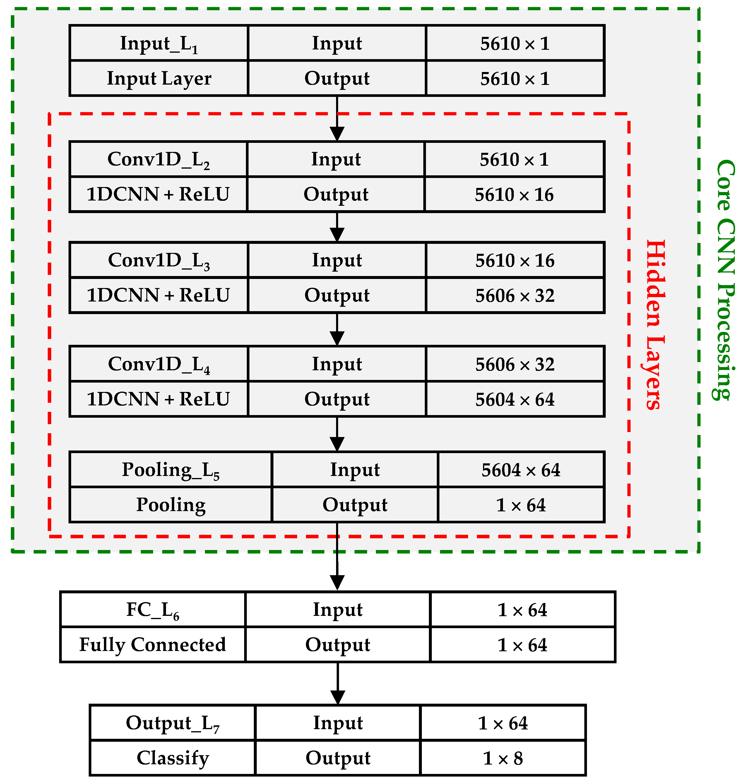
2.6.1. 1D-CNN Architecture

The 1D-CNN architecture used for device discrimination with sub-Nyquist signal responses is shown in Figure 12. The core CNN processing was implemented using four hidden layers, including three 1D-CNN layers (1DCNN) with Rectified Linear Unit (ReLu) activation and one pooling layer. The pooling layer finds the most significant abstract features (fingerprints) for the dense output layer for device classification. The 1DCNN layers are not fully connected and require fewer parameters when compared to fully connected layers. The non-fully connected 1DCNN convolutional layers in Figure 12 share weights among neurons whereas within the fully connected layer every output neuron is connected to every input neuron through a specific set of weights.

Figure 12 shows the 1D-CNN architecture used for device classification using TDO and FDO responses of sub-Nyquist sampled signals. This architecture is based on the generic 1D-CNN architecture detailed in [48]. As shown, the architecture includes seven total layers with the four core CNN processing layers being hidden layers. The 5610 × 1 dimensional input data were processed in the second CNN Conv1D_L₂ layer (first convolutional layer) using N_Cfil = 16 filters with a kernel size of N_Krn = 5 and output a 5606 × 16 feature map. The third CNN Conv1D_L₃ layer (second convolutional layer) utilized N_Cfil = 32 filters and N_Krn = 3 and output a 5604 × 32 feature map. The fourth CNN Conv1D_L₄ layer (third and final convolutional layer) utilized N_Cfil = 64 filters and N_Krn = 3 and a 5602 × 64 feature map. As indicated in Figure 12, all three Conv1D layers use a Rectified Linear Unit (ReLU) activation function.

The feature map output of the final hidden Conv1D_L₄ convolutional layer in Figure 12 is input to the fifth CNN Pooling_L₅ layer. This layer performs global average pooling to accentuate feature rich information used for subsequent device classification. The Pooling_L₅ layer output is input to a fully connected FC_L₆ layer where optimization is performed to enhance class scoring and classification accuracy in the final Output_L₇ layer. The Output_L₇ results are used to form the classification confusion matrix detailed in Section 2.5 and estimate the %C and %CDR percentages.

The algorithm pseudocode for implementing the 1D-CNN processing in Figure 12 is presented in Algorithm 1. As detailed in the code, CNN processing employs dropout and kernel regularization to address issues associated with overfitting and to accelerate data processing. As indicated in Line 1, the learning process was implemented with an N_Lrn = 0.001 learning rate, N_Epc = 40 epochs, and a mini-batch size of N_MB = 32.

Algorithm 1. Algorithm pseudocode for implementing 1D-CNN processing.

1: CNN (trainX, trainY, validationX, validationY, testX, testY, learningrate = 0.001, epoch = 40, batchsize = 32):

2: inputs = shape (datapoints, dimension = 1)

3: model $\leftarrow$ Conv1D (filters = 16, kernels = 5, activation = ReLU) (input)

4: model $\leftarrow$ Conv1D (filters = 32, kernels = 3, activation =ReLU) (model)

5: model $\leftarrow$ Conv1D (filters = 64, kernels = 3, activation = ReLU) (model)

6: model $\leftarrow$ GlobalAvergagePooling (model)

7: model $\leftarrow$ Flatten() (model)

8: model $\leftarrow$ Dropout(0.20) (model)

9: model $\leftarrow$ Dense (neurons = 8, activation = softmax, kernel_regularizer = regularizers.L1L2 (l1 = 1 × 10−5, l2 = 1 × 10−4) (model)

10: model.compile (loss = categorical_crossentropy, optimizer = Adam, learningrate)

11: model. Fit (trainX, trainY, validationX, validationY, epoch, batchsize)

12: Accuracy = model.evaluate (testX, testY)

13: return Accuracy

2.6.2. 2D-CNN Architecture

Figure 13 shows the 2D-CNN architecture used for JTF-based classification. This architecture includes replication of the core 1D-CNN processing layers in Figure 12 with time domain and frequency domain data input separately. The time domain Pooling_${\mathrm{L}}_5^{\mathrm{T}\mathrm{D}}$ and frequency domain Pooling_${\mathrm{L}}_5^{\mathrm{F}\mathrm{D}}$ layer outputs are independently processed within the fully connected FC_L₁₁ and FC_L₁₂ layers, respectively. These fully connected layer outputs are merged within the Concatenate_L₁₃ layer before final Output_L₁₄ classification occurs. The impact of this 2D-CNN JTF processing on the final classification performance is determined by analyzing confusion matrix %C and %CDR percentage estimates.

3. Device Discrimination Results

Classification performance of MDA models representing all N_Cls = 8 devices is first considered in Section 3.1. These results are provided to (1) highlight the effects of Nyquist decimation detailed in Section 2.2 and sub-Nyquist decimation detailed in Section 2.3, and (2) to establish a baseline for subsequent CNN performance results in Section 3.2 that highlight the benefits of CNN processing. As with prior related DNA-based discrimination works [5,7,8,9], classification performance analysis is focused on the %C vs. SNR region neighboring an arbitrary performance benchmark of %C = 90%. Section 3.1 MDA and Section 3.2 CNN classification confusion matrices are used with the ID verification process in Section 2.5.2 to generate the counterfeit detection assessment results in Section 3.3.

3.1. MDA Classification Performance

MDA classification results are presented in Figure 14 for the N_CLS = 8 class discrimination of the N_Dev = 8 WirelessHART adapters in Table 1. Results are presented using fingerprints for WirelessHART signals with no decimation (•), Nyquist decimate-by-5 decimation (•), and sub-Nyquist decimate-by-205 decimation (•). Note that the no decimation (•) results are visually obscured by the overlaid Nyquist decimation (•) results—based on CI_95% confidence intervals the no decimation and Nyquist decimate-by-5 results are statistically equivalent for all SNR considered.

By comparison with the statistically equivalent no decimation (•) and Nyquist decimate-by-5 decimation (•) results, the sub-Nyquist decimate-by-205 decimation (•) results are considerably poorer. Considering the %C = 90 arbitrary benchmark region, poorer performance is reflected in degradation metrics that include (1) a decrease in %C (%C_Δ) that is calculated as %C_Δ ≡ %C_Dec − %C_NonDec ≈ 63.2% − 98.4% ≈ −35.2% at SNR = −9 dB, and (2) an increase SNR (SNR_Δ) calculated as SNR_Δ = SNR_Dec − SNR_NonDec ≈ −3.96 + 12.98 ≈ +9.02 dB at %C = 90%. These degradations are highlighted in Figure 14 at the dotted line values.

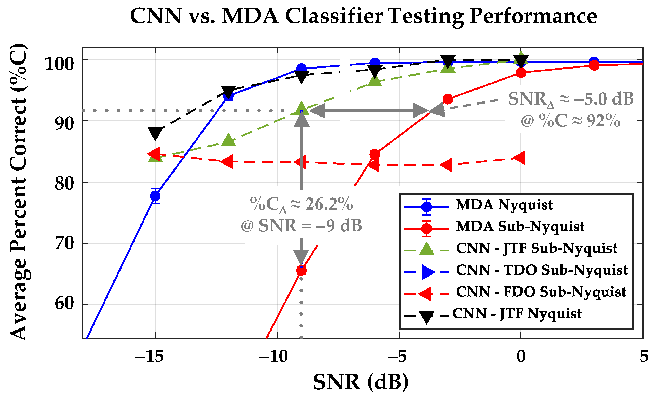
3.2. CNN Classification Performance

CNN classification results are presented in Figure 15 for the N_Dev = 8 WirelessHART adapters in Table 1. This figure shows classification performance of the 1D-CNN Time-Domain-Only (TDO), 1D-CNN Frequency-Domain-Only (FDO) and 2D-CNN Joint Time-Frequency (JTF) architectures overlaid on an expanded region of the MDA %C vs. SNR results in Figure 14. Considering the sub-Nyquist performance results in Figure 15, the 2D-CNN JTF (▲) architecture performance is best overall and includes:

• The %C = 90% benchmark being achieved for SNR ≥ −9 dB;
• A major share of MDA degradation being recovered. This includes the indicated (a) %C_Δ ≡ %C_CNN − %C_MDA ≈ 91.8% − 65.6% ≈ +26.2% improvement at SNR = −9 dB, and (b) SNR_Δ ≡ SNR_CNN − SNR_MDA ≈ −9 – (−4.5) ≈ −5.0 dB improvement at %C ≈ 92%;
• A marginal sub-Nyquist (▲) versus Nyquist (▼) average performance trade-off loss of %C_Δ ≈ −5.6% across the −15 dB ≤ SNR ≤ 0 dB range—considerably more tolerant when considering the MDA %C_Δ ≈ −35.2% loss noted in Figure 14.

3.3. Counterfeit Discrimination Assessment

The estimated %CDRs with ±CI_95% intervals for Figure 14 MDA classification results are summarized in

Table 4. Estimated %CDRs with ±CI_95% intervals for MDA classification results in Figure 14. The Nyquist decimated versus Sub-Nyquist decimated %CDR_Δ differences are provided in the bottom row for comparison and highlight the degrading effects of sub-Nyquist decimation.

	SNR (dB)
	−15.0	−9.0	−3.0	Average
No Decimation	86.4 ± 1.41%	99.1 ± 0.39%	99.7 ± 0.23%	95.1%
Nyquist Decimated	87.0 ± 1.39%	99.2 ± 0.37%	98.8 ± 0.45%	95.0%
Sub-Nyquist Decimated	28.4 ± 0.83%	62.3 ± 0.89%	92.4 ± 0.49%	61.0%
%CDRΔ	−56.6%	−36.9%	−6.4%	−33.3%

for three selected SNR. These %CDRs were calculated using confusion matrices and the estimation process detailed Section 2.5.2. Comparing the No Decimation and Nyquist Decimated estimates in Table 4, there is (1) no statistical difference in %CDR for the SNR = −15 dB and SNR = −9 dB conditions, and (2) less than 1% difference in %CDR for Nyquist decimation at SNR = −3 dB conditions. As reflected in the %CDR_Δ differences in Table 4, there is considerable sub-Nyquist decimation degradation.

The estimated %CDRs with ±CI_95% intervals for Figure 15 CNN sub-Nyquist classification results are summarized in

Table 5. Estimated %CDR with ±CI_95% for Figure 15 CNN classification results. All results for sub-Nyquist decimation with MDA %CDRs taken from Table 4 and reintroduced for comparison.

	SNR (dB)
	−15.0	−9.0	−3.0	Average
CNN TDO	83.1 ± 1.54%	92.3 ± 1.10%	97.3 ± 0.67%	90.9%
CNN FDO	79.5 ± 1.66%	82.3 ± 1.57%	82.8 ± 1.55%	81.5%
CNN JTF	82.2 ± 1.58%	91.5 ± 1.15%	99.2 ± 0.37%	91.0%
MDA	28.4 ± 0.83%	62.3 ± 0.89%	92.4 ± 0.49%	61.0%
JTF vs. MDA %CDRΔ	+53.8%	+29.2%	+6.8%	+29.9%

for three selected SNR. These were calculated using classification confusion matrices for results in Figure 15 and the estimation process detailed in Section 2.5.2. Based on the ±CI_95% intervals, CNN %CDR performance of (1) FDO is the poorest for all SNR, (2) TDO and JTF are statistically equivalent for SNR = −15 dB and SNR = −9 dB, and (3) JTF is marginally better than TDO by %CDR_Δ ≈ 2% at SNR = −3 dB. In light of minimizing computational complexity, it could be argued that the 1D-CNN TDO architecture may be preferred over the 2D-CNN JTF architecture for operational implementation if the %CDR_Δ ≈ 2% performance trade-off is not tolerable.

The corresponding sub-Nyquist MDA results from Table 4 are also provided in Table 5 for comparison. As indicated, the CNN JTF classifier outperforms the MDA classifier by a considerable margin and achieves the arbitrary %CDR > 90% benchmark for all SNR ≥ −9 dB. The CNN JTF classifier improvement relative to MDA is reflected in the %CDR_Δ = %CDR_JTF − %CDR_MDA percentages in the bottom row. Collectively considering %CDR_Δ for the three represented SNR, the CNN JTF classifier provides an average improvement of %CDR_Δ ≈ 29.9% in counterfeit detection performance relative to the MDA classifier, while achieving the %CDR > 90% benchmark for all SNR ≥ −9 dB.

The final counterfeit assessment results are presented in

Table 6. Comparison of estimated counterfeit detection (%CDR), precision (%CPR), and recall (%CRR) metrics for best-case Figure 15 results using the 2D-JTF CNN with sub-Nyquist features.

	SNR (dB)
	−15.0	−9.0	−3.0	Average
%CDR	82.2 ± 1.58%	91.5 ± 1.15%	99.2 ± 0.37%	91.0%
%CPR	87.4 ± 1.37%	93.9 ± 0.99%	99.2 ± 0.37%	93.5%
%CRR	85.4 ± 1.45%	92.9 ± 1.06%	99.5 ± 0.29%	92.6%

to enable performance comparison between the generally less rigorous %CDR detection metric and the alternate more rigorous hypothesis testing %CPR precision and %CRR recall metrics calculated using Equations (1) and (2), respectively. These results show that the cross-SNR average CNN counterfeit detection, precision, and recall rates all exceed 90%.

4. Summary and Conclusions

This work was motivated by the need to achieve reliable detection of counterfeit electronic, electrical, and electromechanical devices being used in critical information and communications technology applications. The counterfeit mitigation goal is to ensure that operational integrity and resiliency objectives are maintained [1,2]. WirelessHART is among the key communications technologies requiring protection and the current motivation for protecting WirelessHART systems is generally unchanged from prior related work [5,7,8,9,10]. One could argue that the motivation today is even stronger than ever given the number of fielded WirelessHART devices is approaching tens of millions [11] and hundreds of thousands of WirelessHART devices enter the supply chain annually [12]. Counterfeit device detection is addressed with a goal of enhancing the operational transition potential of previously demonstrated active DNA fingerprinting methods [8,9]. The goal is addressed in light of increased computational efficiency (decreased computational complexity) and increased counterfeit detection rate objectives.

Computational efficiency can generally be improved by reducing the total number of processed signal samples. This reduction is easily accomplished through sample decimation which is generally applied with a goal of retaining information—this is generally assured when the Nyquist sampling constraint is enforced. Retaining signal information is not a DNA fingerprinting requirement and thus an aggressive NDec = 205 sample decimation was applied to the WirelessHART adapter responses from [8]—this pushed the spectral information content well-below the Nyquist constraint. This resulted in an effective sample rate reduction (1 GSps to 200 MSps) and the desired reduction in the total number of samples (1,150,000 to 230,000) being processed.

The sub-Nyquist decimate-by-205 sampled responses were used for DNA-based Multiple Discriminant Analysis (MDA) and Convolutional Neural Network (CNN) classification. Counterfeit device classification and detectability was performed using eight commercial WirelessHART communication adapters [7,8,9]. The MDA classifier performance provided a baseline for highlighting (1) the overall degrading effects of sub-Nyquist sampling, and (2) detectability improvements that are realized using the CNN classifier. Relative to using Nyquist-compliant DNA fingerprint features, MDA performance using DNA features from sub-Nyquist sampled WirelessHART responses included decreases of %C_Δ ≈ 35.2% and %CDR_Δ ≈ 36.9% in classification and counterfeit detection at SNR = −9 dB. Corresponding CNN classifier performance using the same sub-Nyquist sampled responses was considerably better with a majority of the MDA degradation being recovered. This included best case CNN performance with a 2D Joint Time-Frequency (JTF) CNN architecture providing increases of %C_Δ ≈ 26.2% and %CDR_Δ ≈ 29.2% at SNR = −9 dB. For the full range of −15 dB ≤ SNR ≤ −3 dB average CNN performance included %CDR_Δ ≈ 29.9%, with corresponding detection, precision and recall rates all exceeding 90% for SNR ≥ −9 dB.

References

1. Cyber Security and Infrastructure Agency (CISA). Assessment of the Critical Supply Chains Supporting the U.S. Information and Communications Technology Industry: Overview of Executive Order 14017—America’s Supply Chains. 2021. Available online: https://www.dhs.gov/publication/assessment-critical-supply-chains-supporting-us-ict-industry (accessed on 7 February 2023).
2. U.S. Department of Commerce; U.S. Department of Homeland Security. Assessment of the Critical Supply Chains Supporting the U.S. Information and Communications Technology Industry. Available online: https://www.dhs.gov/sites/default/files/2022-02/ICT%20Supply%20Chain%20Report_2.pdf (accessed on 7 February 2023).
3. FieldComm Group. WirelessHART: Proven and Growing Technology with a Promising Future; Global Control; FieldComm Group: Austin, TX, USA, 2018; Available online: https://tinyurl.com/fcgwirelesshartglobalcontrol (accessed on 7 February 2023).
4. Majid, M.; Habib, S.; Javed, A.R.; Rizwan, M.; Srivastava, G.; Gadekallu, T.R.; Lin, J.C.W. Applications of Wireless Sensor Networks and Internet of Things Frameworks in Industry Revolution 4.0: A Systematic Literature Review. Sensors 2022, 22, 2087. [Google Scholar] [CrossRef] [PubMed]
5. Rondeau, C.M.; Temple, M.A.; Betances, J.A.; Schubert Kabban, C.M. Extending Critical Infrastructure Element Longevity Using Constellation-Based ID Verification. J. Comput. Secur. 2020, 100, 102073. [Google Scholar] [CrossRef]
6. Yang, K.; Forte, D.; Tehranipoor, M.M. CDTA: A Comprehensive Solution for Counterfeit Detection, Traceability, and Authentication in the IoT Supply Chain. ACM Trans. Des. Autom. Electron. Syst. 2017, 22, 42. [Google Scholar] [CrossRef]
7. Gutierrez del Arroyo, J.; Borghetti, B.; Temple, M. Consideration for Radio Frequency Fingerprinting Across Multiple Frequency Channels. Sensors 2022, 22, 2111. [Google Scholar] [CrossRef]
8. Maier, M.J.; Hayden, H.S.; Temple, M.A.; Fickus, M.C. Ensuring the Longevity of WirelessHART Devices in Industrial Automation and Control Systems Using Distinct Native Attribute Fingerprinting. Int. J. Crit. Infrastruct. Prot. 2022. Under Review. [Google Scholar]
9. Mims, W.H.; Temple, M.A.; Mills, R.A. Active 2D-DNA Fingerprinting of WirelessHART Adapters to Ensure Operational Integrity in Industrial Systems, MDPI. Sensors 2022, 22, 4906. [Google Scholar] [CrossRef]
10. Rondeau, C.M.; Temple, M.A.; Schubert Kabban, C.M. TD-DNA Feature Selection for Discriminating WirelessHART IIoT Devices. In Proceedings of the 53rd Hawaii International Conference on System Sciences (HICSS), Maui, HI, USA, 7–10 January 2020. Available online: https://scholarspace.manoa.hawaii.edu/bitstreams/35252979-27c2-4ae0-b8fb-35529f731e5a/download (accessed on 7 February 2023).
11. Devan, P.A.M.; Hussin, F.A.; Ibrahim, R.; Bingi, K.; Khanday, F.A. A Survey on the Application of WirelessHART for Industrial Process Monitoring and Control. Sensors 2021, 21, 4951. [Google Scholar] [CrossRef] [PubMed]
12. FieldComm Group. WirelessHART User Case Studies; Technical Report; FieldComm Group: Austin, TX, USA, 2019; Available online: https://tinyurl.com/fcgwirelesscs (accessed on 7 February 2023).
13. Cyber Security and Infrastructure Agency (CISA). Cybersecurity and Physical Security Convergence. 2021. Available online: https://www.cisa.gov/cybersecurity-and-physical-security-convergence (accessed on 7 February 2023).
14. Society of Automobile Engineers (SAE). Counterfeit Electrical, Electronic, and Electromechanical (EEE) Parts; Avoidance, Detection, Mitigation, and Disposition, Issued: 4 April 2009. Available online: https://standards.globalspec.com/std/14217318/SAE%20AS6462 (accessed on 7 February 2023).
15. Society of Automobile Engineers (SAE). Counterfeit Electrical, Electronic, and Electromechanical (EEE) Parts; Avoidance, Detection, Mitigation, and Disposition Verification Criteria, Doc ID: SAE-AS6462, Quick Search, Last Update: 10 January 2023. Available online: https://quicksearch.dla.mil/qsDocDetails.aspx?ident_number=280435 (accessed on 7 February 2023).
16. Society of Automobile Engineers (SAE). Counterfeit Electrical, Electronic, and Electromechanical (EEE) Parts; Avoidance, Detection, Mitigation, and Disposition, Latest Revision: 14 April 2022. Available online: https://www.sae.org/standards/content/as5553d/ (accessed on 7 February 2023).
17. Raut, R.D.; Gotmare, A.; Narkhede, B.E.; Govindarajan, U.H.; Bokade, S.U. Enabling Technologies for Industry 4.0 Manufacturing and Supply Chain: Concepts, Current Status, and Adoption Challenges. IEEE Eng. Manag. Rev. 2020, 48, 83–102. [Google Scholar] [CrossRef]
18. Voetberg, B.; Carbino, T.; Temple, M.; Buskohl, P.; Denault, J.; Glavin, N. Evolution of DNA Fingerprinting for Discriminating Conductive Ink Specimens. In Proceedings of the Digest Abstract, 2019 Government Microcircuit Applications & Critical Technology Conference (GOMACTech), Albuquerque, NM, USA, 25–28 March 2019. [Google Scholar]
19. Lukacs, M.W.; Zeqolari, A.J.; Collins, P.J.; Temple, M.A. RF-DNA Fingerprinting for Antenna Classification. IEEE Antennas Wirel. Propag. Lett. 2015, 14, 1455–1458. [Google Scholar] [CrossRef]
20. Maier, M.J.; Temple, M.A.; Betances, J.A.; Fickus, M.C. Active Distinct Native Attribute (DNA) Fingerprinting to Improve Electrical, Electronic, and Electromechanical (EEE) Component Trust. In Proceedings of the Digest Abstract, 2022 Government Microcircuit Applications & Critical Technology Conference (GOMACTech), Maimi, FL, USA, 21–24 March 2022. [Google Scholar]
21. Paul, A.J.; Collins, P.J.; Temple, M.A. Enhancing Microwave System Health Assessment Using Artificial Neural Networks. IEEE Antennas Wirel. Propag. Lett. 2019, 18, 2230–2234. [Google Scholar] [CrossRef]
22. Siemens. WirelessHART Adapter, SITRANS AW210, 7MP3111, User Manual; Siemens: Munich, Germany, 2012; Available online: https://tinyurl.com/yyjbgybm (accessed on 7 February 2023).
23. Pepperl+Fuchs. WHA-BLT-F9D0-N-A0-*, WirelessHART Adapter, Manual. Available online: https://tinyurl.com/pepplusfucwirelesshart (accessed on 7 February 2023).
24. Soltanieh, N.; Norouzi, Y.; Yang, Y.; Karmakar, N.C. A Review of Radio Frequency Fingerprinting Techniques. IEEE J. Radio Freq. Identif. 2022, 4, 222–233. [Google Scholar] [CrossRef]
25. Chen, X.; Sobhy, E.A.; Yu, Z.; Hoyos, S.; Silva-Martinez, J.; Palermo, S.; Sadler, B.M. A Sub-Nyquist Rate Compressive Sensing Data Acquisition Front-End. IEEE J. Emerg. Sel. Top. Circuits Syst. 2012, 2, 542–551. [Google Scholar] [CrossRef]
26. Brunelli, D.M.; Caione, C. Sparse Recovery Optimization in Wireless Sensor Networks with a Sub-Nyquist Sampling Rate. Sensors 2015, 15, 16654–16673. [Google Scholar] [CrossRef]
27. Deng, W.; Jiang, M.; Dong, Y. Recovery of Undersampled Signals Based on Compressed Sensing. In Proceedings of the 2019 IEEE 4th International Conference on Signal and Image Processing (ICSIP), Wuxi, China, 19–21 July 2019; pp. 636–640. [Google Scholar] [CrossRef]
28. Fang, J.; Wang, B.; Li, H.; Liang, Y.C. Recent Advances on Sub-Nyquist Sampling-Based Wideband Spectrum Sensing. IEEE Wirel. Commun. Mag. 2021, 28, 115–121. [Google Scholar] [CrossRef]
29. Keysight Technologies. PNA Family Microwave Network Analyzer (N522x/3x/4xB), Configuration Guide, Doc ID: 5992-1465EN. 10 September 2021. Available online: https://www.keysight.com/us/en/assets/7018-05185/configuration-guides/5992-1465.pdf (accessed on 7 February 2023).
30. LeCroy. WaveMaster® 8 Zi-A Series: 4 GHz-45GHz Doc ID: WM8Zi-A-DS-09May11. 2011. Available online: https://docs.rs-online.com/035e/0900766b8127e31c.pdf (accessed on 7 February 2023).
31. Reising, D.R.; Temple, M.A. WiMAX Mobile Subscriber Verification Using Gabor-Based RF-DNA Fingerprints. In Proceedings of the IEEE International Conference on Communications (ICC), Ottawa, ON, Canada, 10–15 June 2012. [Google Scholar] [CrossRef]
32. Talbot, C.M.; Temple, M.A.; Carbino, T.J.; Betances, J.A. Detecting Rogue Attacks on Commercial Wireless Insteon Home Automation Systems. J. Comput. Secur. 2018, 74, 296–307. [Google Scholar] [CrossRef]
33. Soberon, A.; Stute, W. Assessing Skewness, Kurtosis and Normality in Linear Mixed Models. J. Multivar. Anal. 2017, 161, 123–140. [Google Scholar] [CrossRef]
34. Tharwat, A. Classification Assessment Methods. Appl. Comput. Inform. 2020, 17, 168–192. [Google Scholar] [CrossRef]
35. Park, H.; Leemis, L.M. Ensemble Confidence Intervals for Binomial Proportions. Stat. Med. 2019, 38, 3460–3475. [Google Scholar] [CrossRef]
36. Memon, N.; Parikh, H.; Patel, S.; Patel, D.; Patel, V. Automatic Land Cover Classification of Multi-resolution Dualpol Data Using Convolutional Neural Network Remote Sensing Applications. Soc. Environ. 2021, 22, 100491. [Google Scholar]
37. Shi, F.; Zhao, C.; Zhao, X.; Zhou, X.; Li, X.; Zhu, J. Spatial Variability of the Groundwater Exploitation Potential in an Arid Alluvial-Diluvial Plain using GIS-based Dempster-Shafer Theory. Quat. Int. 2021, 571, 127–135. [Google Scholar] [CrossRef]
38. Tegegne, A.M. Applications of Convolutional Neural Network for Classification of Land Cover and Groundwater Potentiality Zones. J. Eng. 2022, 2022, 6372089. [Google Scholar] [CrossRef]
39. Rituraj, R.; Ecker, D. A Comprehensive Investigation into the Application of Convolutional Neural Networks (ConvNet/CNN) in Smart Grids, 17 November 2022. Available online: https://papers.ssrn.com/sol3/papers.cfm?abstract_id=4279873 (accessed on 7 February 2023).
40. Emmanuel, S.; Onuodu, F.E. Object Detection Using Convolutional Neural Network Transfer Learning. Int. J. Innov. Res. Eng. Multidiscip. Phys. Sci. 2022, 10. Available online: https://www.ijirmps.org/papers/2022/3/1371.pdf (accessed on 7 February 2023).
41. Nasiri, F.; Hamidouche, W.; Morin, L.; Dhollande, N.; Cocherel, G. Prediction-Aware Quality Enhancement of VVC Using CNN. In Proceedings of the IEEE International Conference on Visual Communications and Image Processing (VCIP), Macau, China, 1–4 December 2020. [Google Scholar] [CrossRef]
42. Huang, J.; Huang, S.; Zeng, Y.; Chen, H.; Chang, S.; Zhang, Y. Hierarchical Digital Modulation Classification Using Cascaded Convolutional Neural Network. J. Commun. Inf. Netw. 2021, 6, 72–81. [Google Scholar] [CrossRef]
43. Atik, I. Classification of Electronic Components Based on Convolutional Neural Network Architecture. Energies 2022, 15, 2347. [Google Scholar] [CrossRef]
44. Li, J.; Li, W.; Chen, Y.; Gu, J. A PCB Electronic Components Detection Network Design Based on Effective Receptive Field Size and Anchor Size Matching. J. Comput. Intell. Neurosci. 2021, 2021, 6682710. [Google Scholar] [CrossRef]
45. Rumelhart, D.E.; Hinton, G.; Williams, R.J. Learning Representations by Back-Propagation Errors. Nature 1986, 323, 533–536. [Google Scholar] [CrossRef]
46. Kiranyaz, S.; Avci, O.; Abdeljaber, O.; Ince, T.; Gabbouj, M.; Inman, D.J. 1D Convolutional Neural Networks and Applications: A survey. Mech. Syst. Signal Process. 2021, 151, 107398. [Google Scholar] [CrossRef]
47. Geron, A. Hands-on Machine Learning with Scikit-Learn, Keras & TensorFlow, 2nd ed.; O’Reilly: Sebastopol, CA, USA, 2019. [Google Scholar]
48. Shoelson, B. Deep Learning in Matlab: A Brief Overiew. In Proceedings of the Mathworks Automotive Conference (MICHauto), Plymouth, MI, USA, 2 May 2018; Available online: https://tinyurl.com/3fy2ax5b (accessed on 7 February 2023).
Figure 1. Active DNA fingerprinting setup used for collecting WirelessHART device responses. Post-collection processing applied prior to DNA fingerprinting.
Electronics 12 01973 g001
Figure 2. Overall down-conversion, filtering, Nyquist decimation, and SNR scaling processes used to generate the desired analysis sA(t) for DNA fingerprinting.
Electronics 12 01973 g002
Figure 3. Time domain amplitude responses for (a) a representative post-collection processed pulse at fS = 1 GSps and (b) the corresponding NDecFac = 5 Nyquist decimated pulse at fS = 200 MSps showing the DNA fingerprinting ROI sample range.
Electronics 12 01973 g003aElectronics 12 01973 g003b
Figure 4. Overlay of Post-Collected (PC) input, Down-Converted (D/C) Image, D/C Filtered, and BandPass filtered (WBP) impulse response (dashed line).
Electronics 12 01973 g004
Figure 5. Overall sub-Nyquist decimation, estimation, filtering, and SNR scaling processes used to generate the desired analysis sA(t) that is input to the DNA fingerprinting process.
Electronics 12 01973 g005
Figure 6. Time domain amplitude responses for (a) a representative post-collection processed pulse at fS = 1 GSps and (b) the corresponding NDecFac = 205 sub-Nyquist decimated pulse response fSDec = 1/205 GSps showing the DNA fingerprinting ROI sample range.
Electronics 12 01973 g006aElectronics 12 01973 g006b
Figure 7. Overlay of individual SFM sub-pulse (SP) power spectral density (PSD) responses for pulses in Figure 6 with approximate SFM bandwidths bounded by the vertical dashed lines. (a) Post-collected SFM sub-pulse (SP) responses spanning WSFM ≈ 50 MHz. (b) Corresponding NDecFac = 205 sub-pulse (SP) responses spanning WDec ≈ 1 MHz.
Electronics 12 01973 g007aElectronics 12 01973 g007b
Figure 8. Composite SFM power spectral density responses showing spectral regions used to estimate average background noise powers. (a) Post-collected (PC) composite SFM pulse power spectral density with WPC ≈ 50 MHz. Estimates made within WPC include SPC + NPC ≈ 78.74, NPC ≈ 5.54 × 10⁻⁵ and SNRPC ≈ 61.53 dB. (b) Corresponding NDecFac = 205 decimated pulse power spectral density with WSFM ≈ 1 MHz. Estimates made within WSFM include SDec + NDec ≈ 69.92.74, NDec ≈ 3.56 and SNRDec ≈ 12.71 dB.
Electronics 12 01973 g008aElectronics 12 01973 g008b
Figure 9. Time domain effects of Figure 5 processing showing (Top) an input NDecFact = 205 decimated signal sD(t) at SNRDec ≈ 12.71 dB and (Bottom) corresponding output analysis sA(t) signal at SNRA ≈ 0 dB. Non-normalized plots are provided with the same vertical amplitude scale to highlight the effects of SNR degradation due to adding like-filtered AWGN.
Electronics 12 01973 g009
Figure 10. Frequency domain effects of Figure 5 processing showing normalized power spectral density (PSD) for (Top) input NDecFact = 205 decimated signal sD(t) at SNRDec ≈ 12.71 dB and (Bottom) corresponding bandpass filtered analysis signal sA(t) at SNRA ≈ 0 dB. Normalized plots are provided with the same vertical scale to highlight the effects of within band SNR degradation.
Electronics 12 01973 g010
Figure 11. Time domain magnitude response for Figure 9 pulse showing the selected ROI (samples between the red dashed lines) and division into NSrgn = 18 subregions (samples between adjacent red dotted lines) used for generating statistical time domain DNA fingerprint features.
Electronics 12 01973 g011
Figure 12. 1D-CNN architecture used for time-domain-only and frequency-domain-only WirlessHART device classification. The gray shaded box includes core hidden layer and input layer processing elements that are common with the 2D-CNN architecture in Figure 13.
Electronics 12 01973 g012
Figure 13. 2D-CNN architecture used for Joint-Time-Frequency (JTF) domain WirelessHART device classification. The two Core CNN Processing blocks are independent and functionally equivalent to those shown in Figure 12.
Electronics 12 01973 g013
Figure 14. MDA classification using fingerprints for WirelessHART signals with no decimation (), NDecFac = 5 Nyquist decimation () and NDecFac = 205 sub-Nyquist decimation (). The sub-Nyquist SNR (SNRΔ) and %C (%CΔ) degradations are highlighted at the dotted line values.
Electronics 12 01973 g014
Figure 15. MDA vs. CNN classification highlighting the benefits of CNN processing. The 2D-CNN JTF () %CΔ and SNRΔ benefits are highlighted at the dotted line values and represent recovery of MDA classification degradation resulting from sub-Nyquist response decimation.
Electronics 12 01973 g015