
IoT System for Gluten Prediction in Flour Samples Using NIRS Technology, Deep and Machine Learning Techniques

 ,
,  , and
, and 
Abstract
1. Introduction
2. Materials and Methods
2.1. Data Preparation
2.2. Implementation
Hardware and Software Description
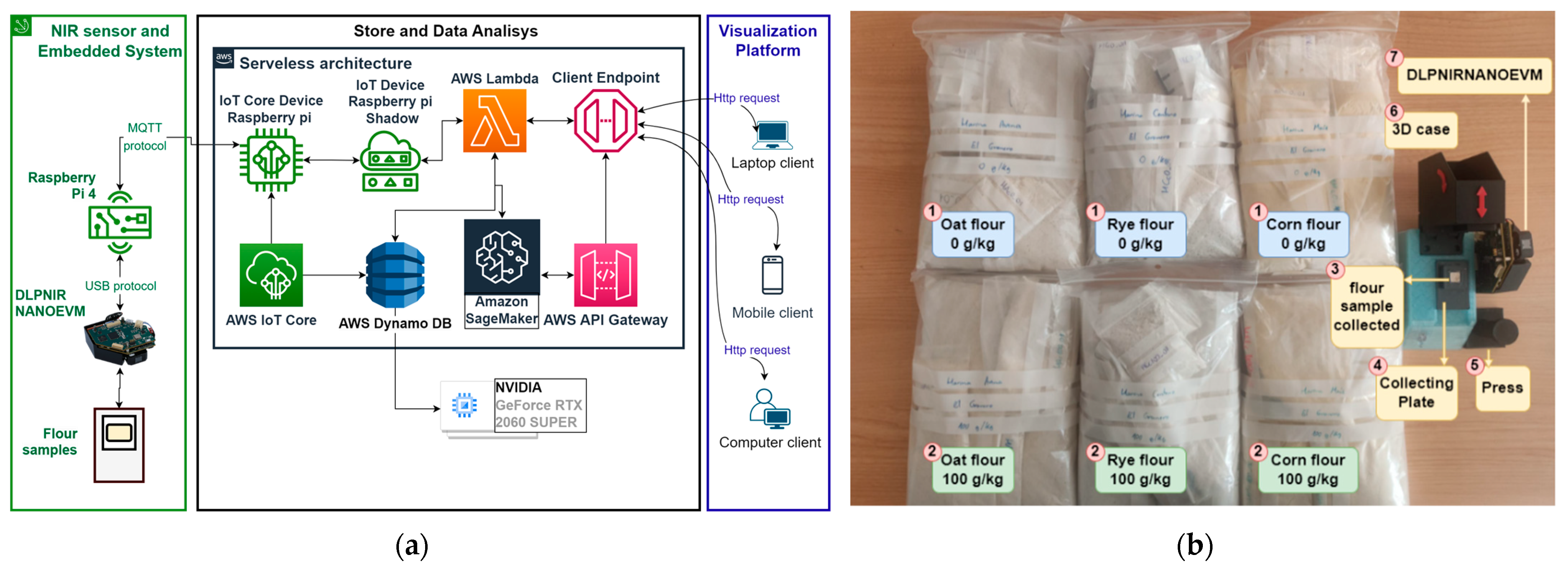
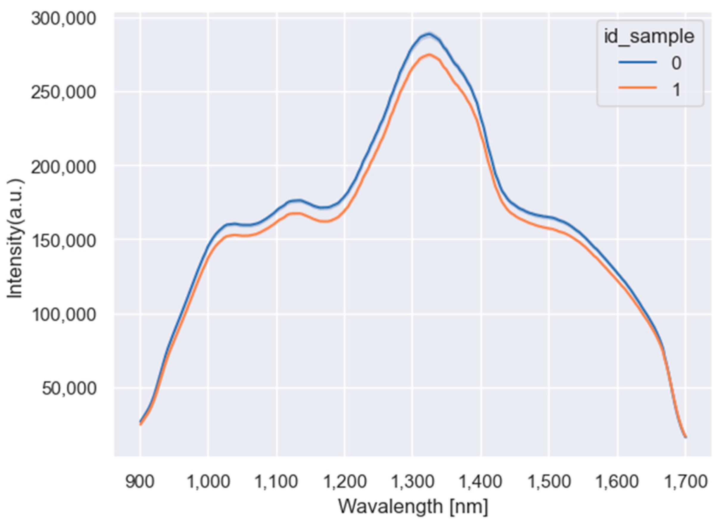
- NIRS sensor and embedded system: as seen in Figure 1a, the IoT prototype portable solution is composed of a Raspberry Pi 4 (Raspberry Pi is a small and low-cost computer, which uses a screen a keyboard, and a mouse and can be used by people of all ages to learn how to program in programming languages as Scratch and Python [32]) and the DLPNIRNANOEVM a compacted evaluation module used for NIRS [33]. The DLPNIRNANOEVM sensor works in the 900–1700 nm wavelength range with a resolution of 4 nm, so one measure provides a total of 228 variables. The output of the sensor was the intensity. The DLPNIRNANOEVM sensor was connected to the Raspberry Pi 4 using the USB protocol and Python scripts were designed for collecting data from the flour samples. To activate the sensor, we created an HTTP endpoint for receiving different requests using JSON files. This endpoint receives different information, including the sensor’s name and id, as well as the action to execute, with different parameters such as the sensor’s state and the duration of data collection. The endpoint then enables an AWS lambda function that changes the status of the shadow in the AWS IoT microservice, which initiates data collection using the Message Queuing Telemetry Transport (MQTT) protocol (MQTT is a standard messaging protocol based on publish/subscribe messaging communication which is ideal for connecting remote devices [34]).
- Data storing and data analysis: the data was received by AWS IoT and forwarded to AWS Lambda, which had several functionalities: managing the logic requests to the database, making the ML and DL predictions, and exposing the endpoints to the final user (client). The data was stored using AWS DynamoDB. The full explanation of this architecture is given in [35].
- For the data analysis, we employed ML and DL algorithms programmed using Python programming language, version 3.9. On the one hand, the ML techniques were trained using the ml.m4.xlarge instance available in AWS sagemaker [36] equipped with 4vCPU and 16 GiB. On the other hand, the DL models were trained using a local machine equipped with an NVIDIA GeForce RTX 2060 SUPER graphic card with 8 GB of VRAM memory and 16 GB of shared GPU memory. We trained the DL algorithms in an eVida local machine to take advantage of the power of the graphic card but also because this made it easier to manipulate the system files, something useful for a custom tuning methodology later explained.
- Visualization platform: it was designed using the Django framework and is communicated with the AWS platform using HTTP requests. The functionalities of this platform are the visualization of gluten measures, the collection of new samples, and the visualization of new predictions. It is worth mentioning that the explanation of the visualization platform is out of the scope of this study, therefore, we do not go into details.
2.3. Data Collection Procedure
- For each new measurement, the operator had to change the collecting plate (grams capacity ≈ 400 mg) (4 in Figure 1b) and then take the flour samples from different locations of the bag (1 or 2 in the same figure). Hence, he/she scooped flour from the top, bottom, center, and lateral sides of the bag to randomize the data collection process as much as possible. Finally, the operator put the samples in the collecting plate (4 in Figure 1b).
- Once the sample was on the collecting plate, the operator smashed the flour trying to keep it on a smooth surface. This was because, after some experiments, we realized that when the surface was not smooth, the data collection was not consistent.
- To avoid cross-contamination of the samples, the operator had to wear different gloves when collecting the data from different flour types. Furthermore, it was necessary to use different spoons and collecting plates for each type of flour. The gloves were thrown away at the end of the day.
- The time collection per sample was approximately 30 s, during this time window, the DLPNIRNANOEVM sensor measured the exposed sample and forwarded the data to the AWS platform.
- All the samples were collected with the same sensor and embedded system. Therefore, to measure the data it was necessary to design and print a 3D mechanical system. On the right in Figure 1b the 3D mechanical system is shown, it is composed of a 3d black case at the top (it contains the DLPNIRNANOEVM inside) and the blue box at the bottom (it contains the Raspberry Pi 4). It was used to keep the sensor rigid during the measuring process, but also to collect the data in a dark environment.
2.4. Classification Framework
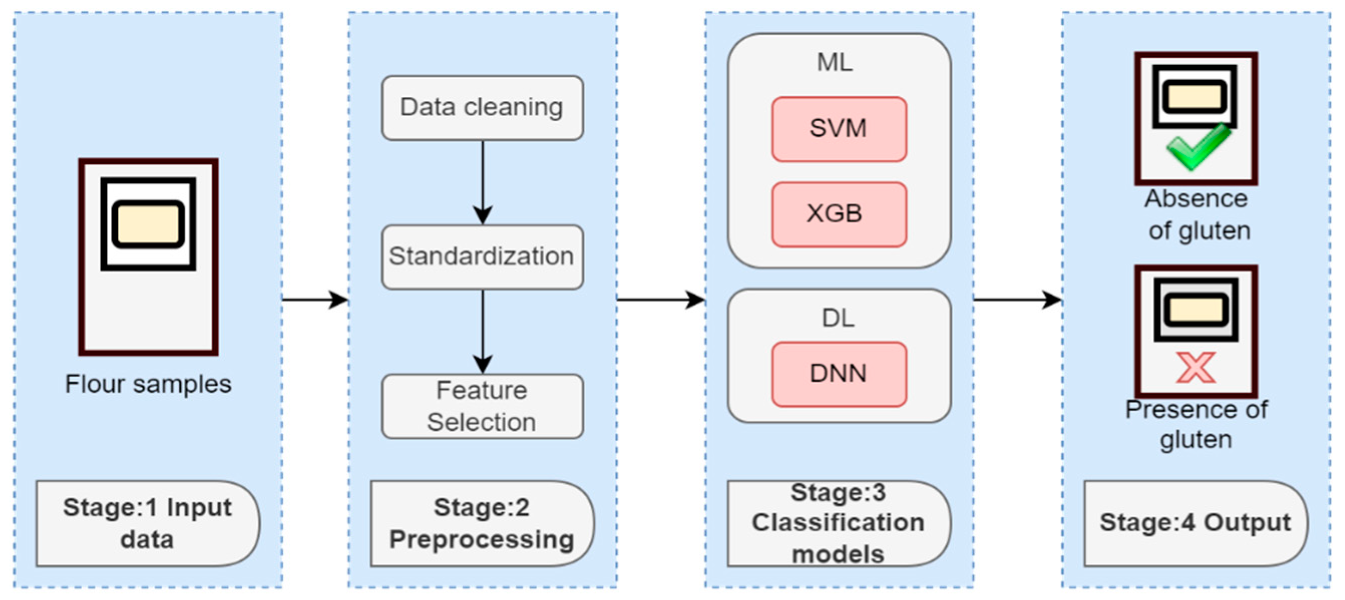
2.4.1. Input Data
2.4.2. Preprocessing
- Data cleaning: Despite the good quality of the data provided by the DLPNIRNANOEVM sensor, we checked that it met the following requirements. First, we checked the valid data, looking at whether the variable names and values met the required formats. Second, we checked the complete data, looking for NaN values and replacing them with valid values. Third, we checked the consistent data, looking at the outlier values in the dataset. Finally, we checked the unique data deleting the duplicate values.
- Standardization: once we cleaned the data, the next step was applying the standardization of the data. We applied row standardization, given the fact that all the columns had the same unit. During this process, the variables were standardized by removing the mean and scaling to unit variance [37]. The standard score is given by (1).
- Feature selection: We selected the 3 wavelength ranges to train the ML and DL algorithms: 1089–1325 nm; 1239–1353 nm and 1422–1583 nm; and the whole spectrum 900–1700 nm, based on our previous study [31]. The purpose was to corroborate the possibility of predicting the presence or absence of gluten in the flour by only selecting some of the wavelength variables.
2.4.3. Classification Models
2.4.3.1. Support Vector Machine
2.4.3.2. Extreme Gradient Boosting (XGBoost)
2.4.3.3. Deep Neural Network
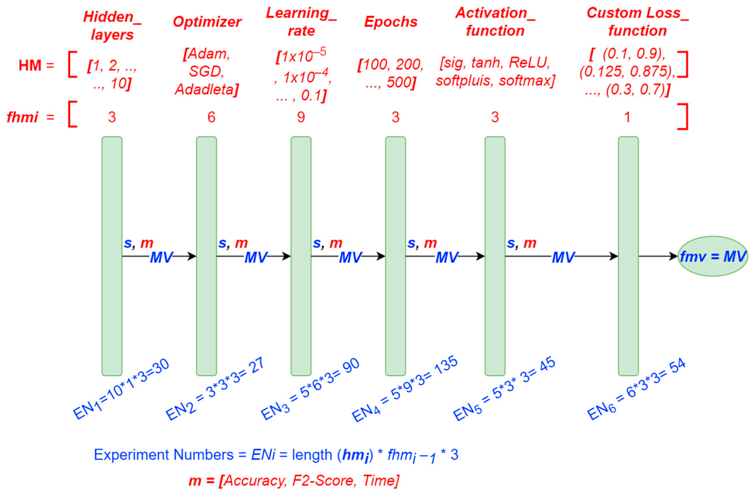
2.4.3.4. Hyperparameter Tuning Methodology for DNN
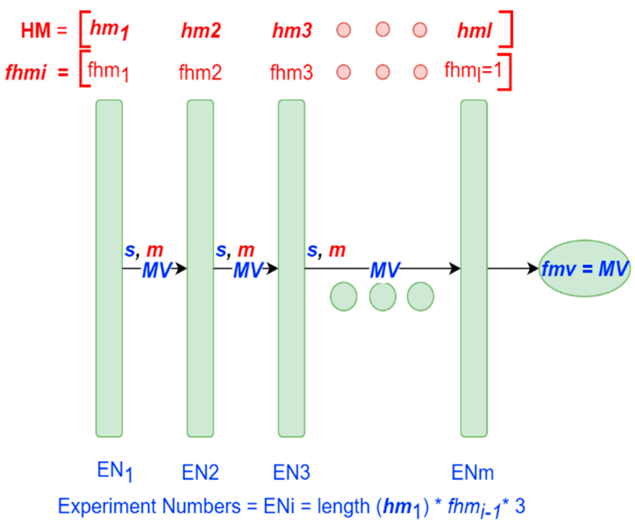
- Hyperparameters Matrix (): it is a matrix of hyperparameters and its values. The hyperparameters will be tuned in the row (i) order indicated.
- Filter (): it is a vector (for each hyperparameter) of thresholds that limit the number of models that pass to the next iteration (See Table 2, step 3.1.2).
- Metrics (m): it is a vector of the metrics to evaluate the performance of the models. The metrics will determine the score for each model.
- Model values (): it is a matrix that contains the best hyperparameter values for each model selected during each iteration. (See Table 2, step 3.2).
- Final model values (): it is a vector of the hyperparameter values for the best model selected at the end of the process.
- Score(): it is a vector of the scores for each ij iteration. The vector is rewritten for each j iteration.
- Random vector (): it is a random vector.
- where i is the hyperparameter iterated, j is the respective values, l is the number of hyperparameters, and n is the number of hyperparameter values. Furthermore, we followed the matrix notation: the matrixes are in capital letters and bolded, the vectors are in lowercase and bolded, and the scalars are in lowercase.
2.4.4. Output
3. Results
3.1. Machine Learning Hyperparameter Tuning
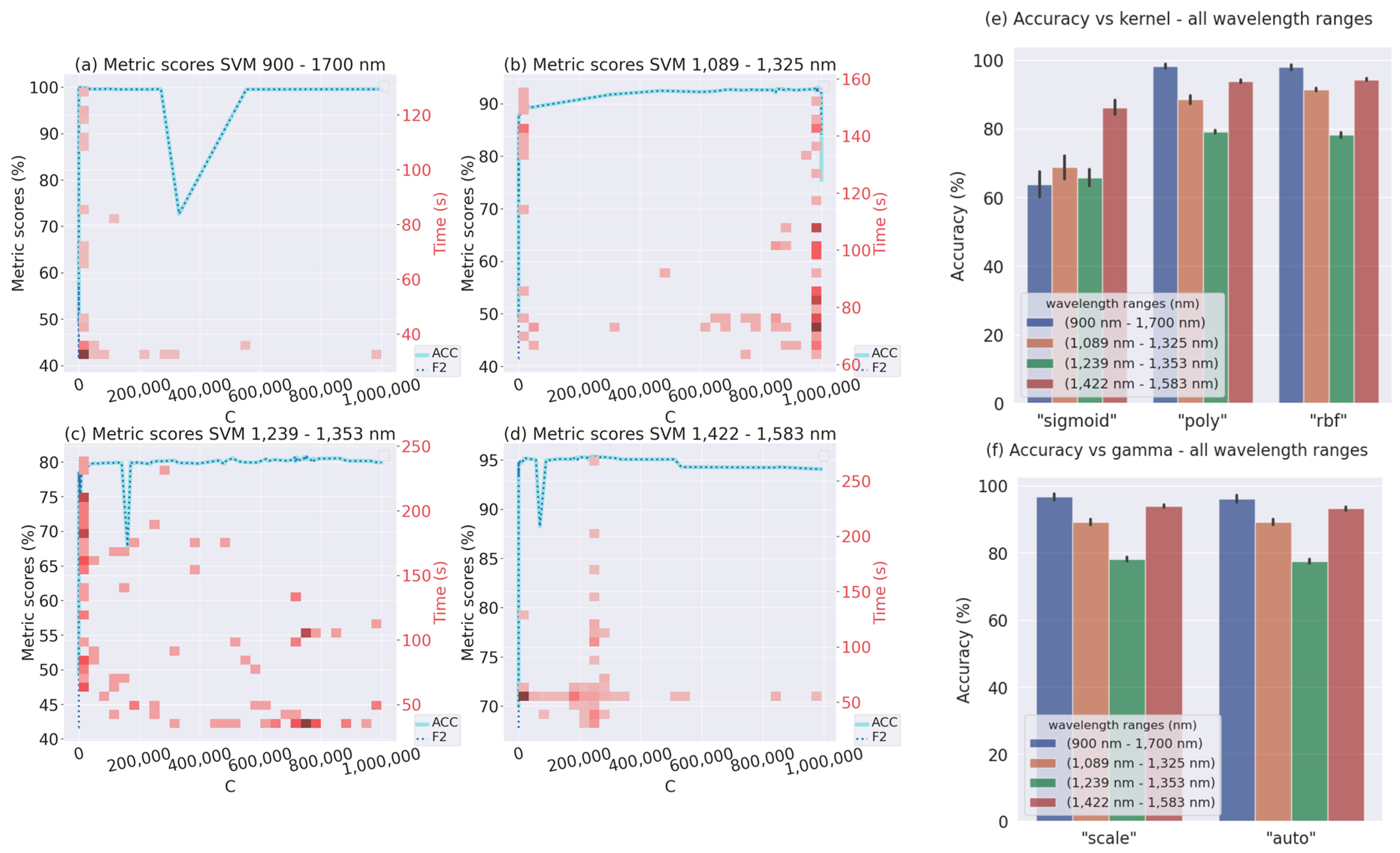
3.1.1. SVM
3.1.2. XGBoost
3.2. Deep Learning Hyperparameter Tuning
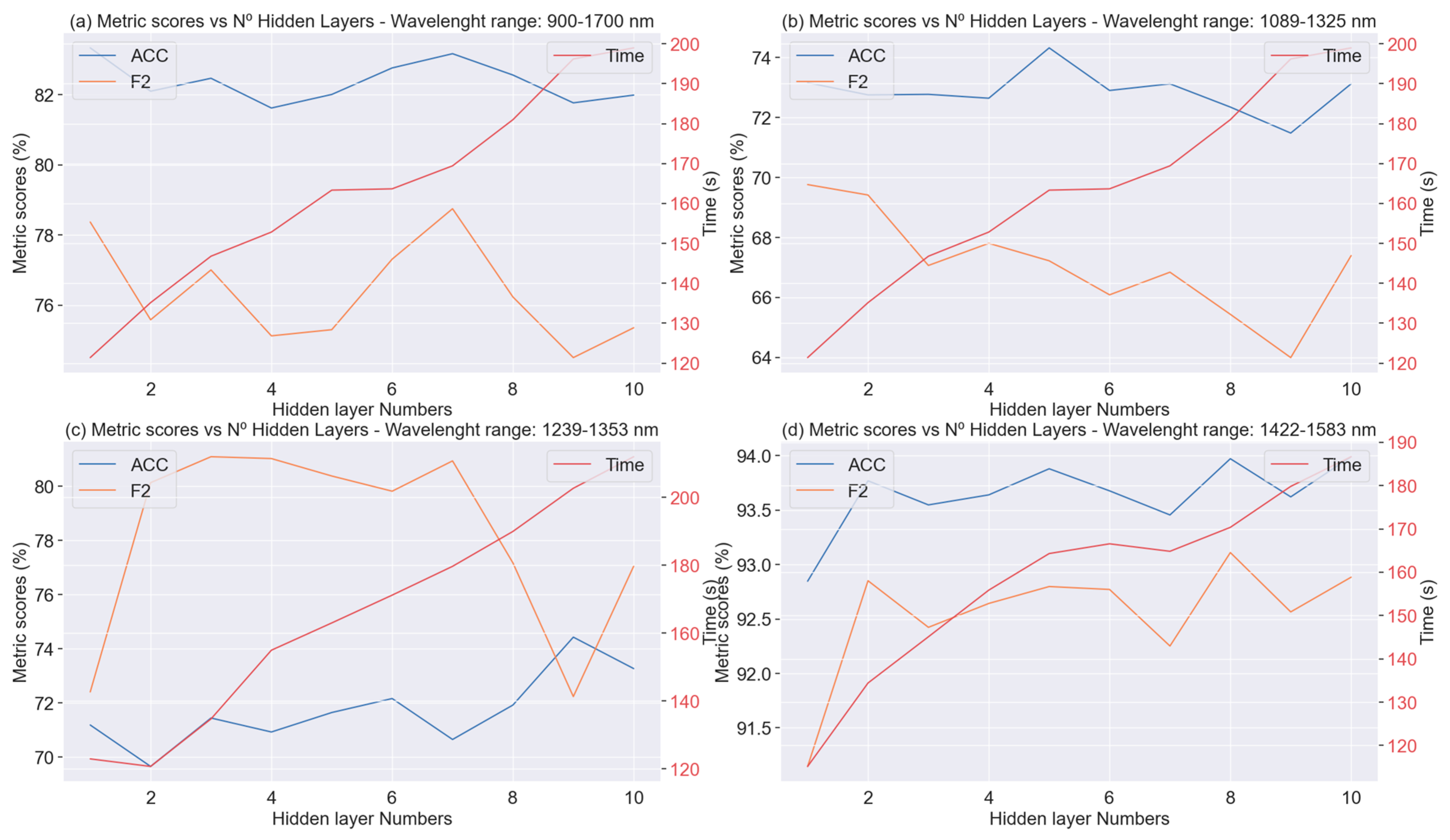
- Hidden layers
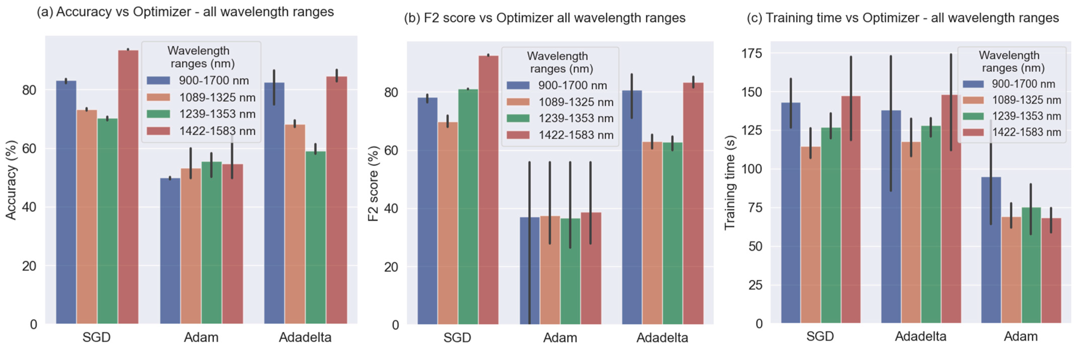
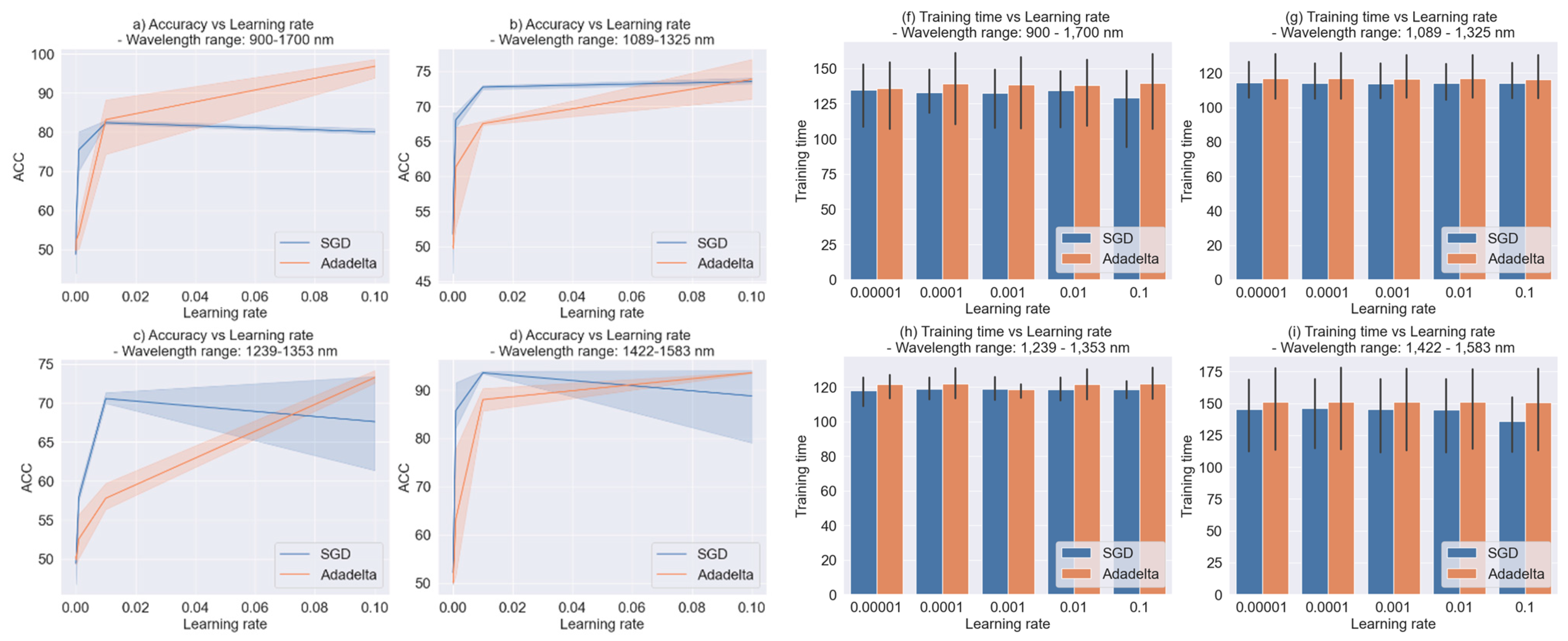
- Optimizer
- Learning rate
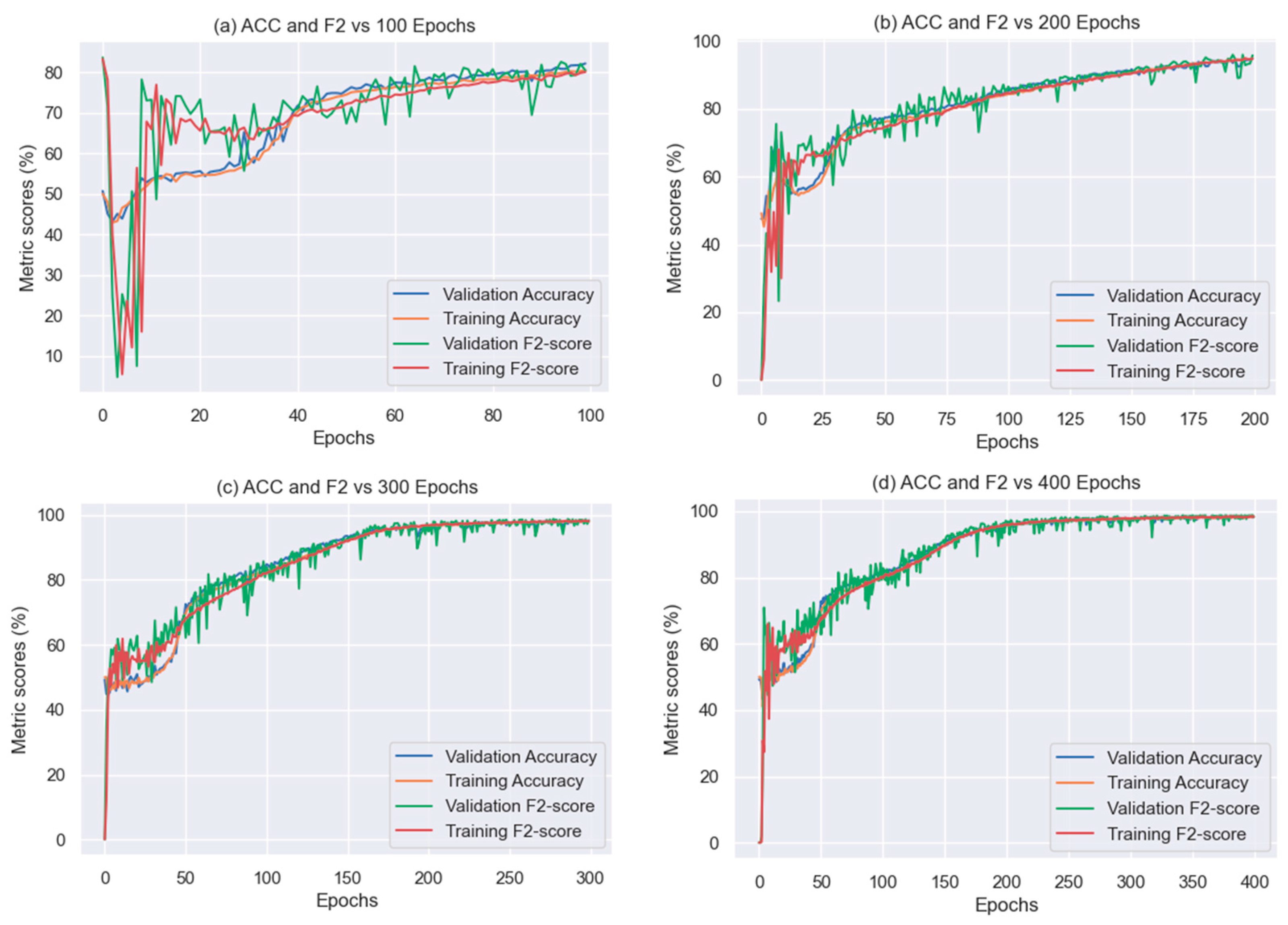
- Epochs
- Activation function
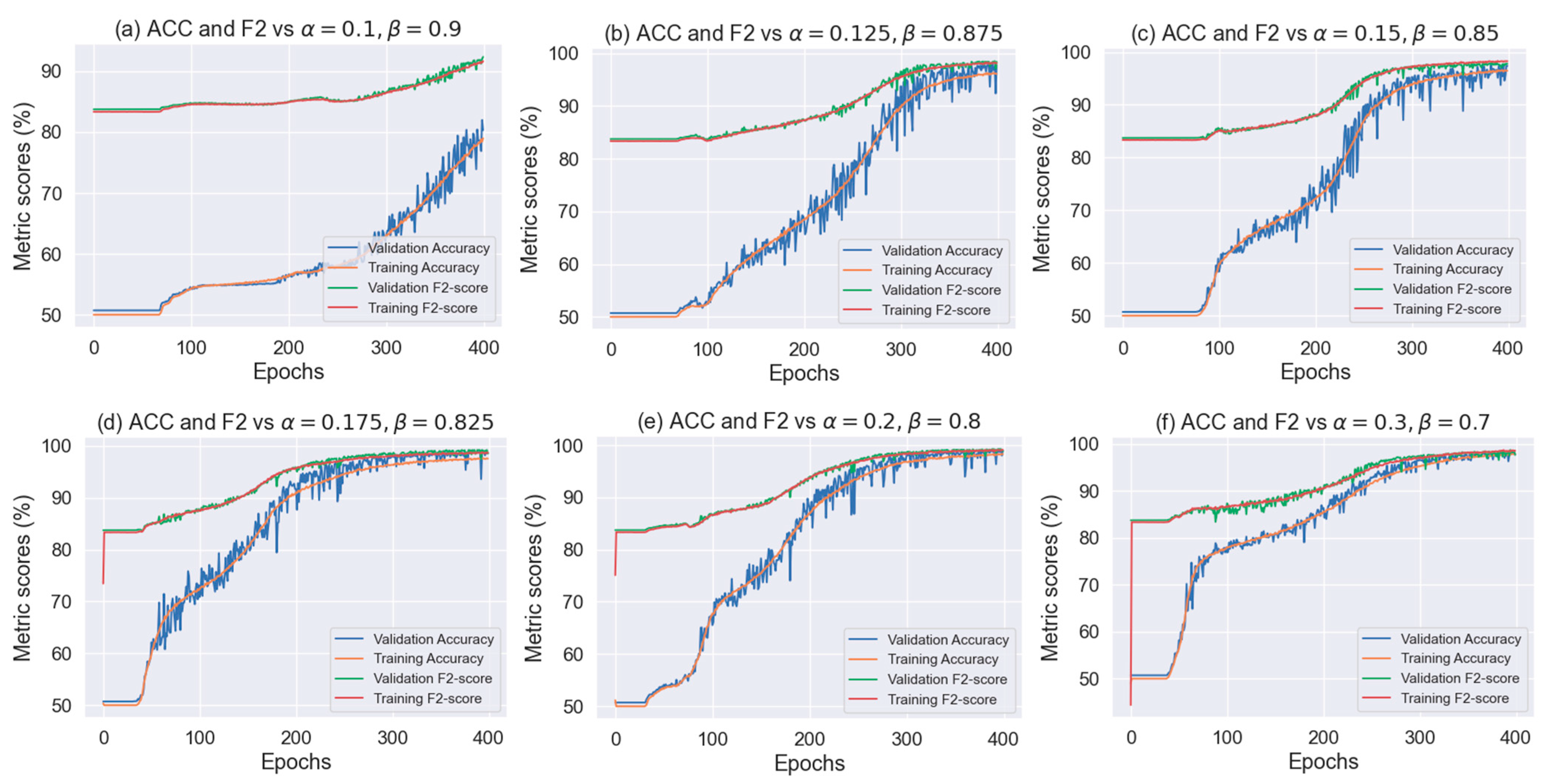
- Loss function
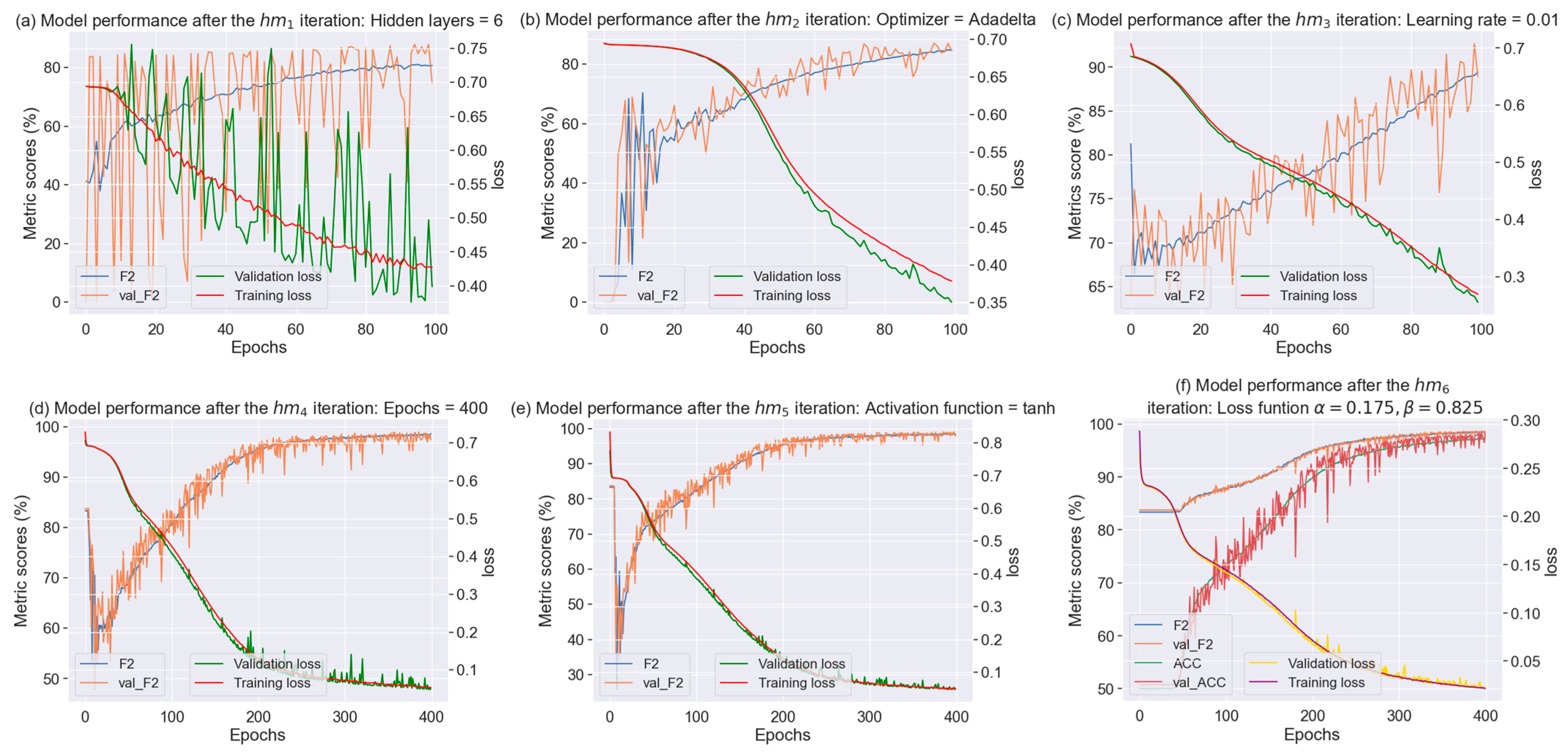
- Summary of the proposed tuning methodology
3.3. Classification Results
4. Discussion and Conclusions
Author Contributions
Funding
Data Availability Statement
Acknowledgments
Conflicts of Interest
References
- Schalk, K.; Lexhaller, B.; Koehler, P.; Scherf, K. Isolation and Characterization of Gluten Protein Types from Wheat, Rye, Barley and Oats for Use as Reference Materials. PLoS ONE 2017, 12, e0172819. [Google Scholar] [CrossRef] [PubMed]
- Calabriso, N.; Scoditti, E.; Massaro, M.; Maffia, M.; Chieppa, M.; Laddomada, B.; Carluccio, M.A. Non-Celiac Gluten Sensitivity and Protective Role of Dietary Polyphenols. Nutrients 2022, 14, 2679. [Google Scholar] [CrossRef] [PubMed]
- Akhondi, H.; Ross, A.B. Gluten Associated Medical Problems. In StatPearls; StatPearls Publishing: Treasure Island, FL, USA, 2022. [Google Scholar]
- Klemm, N.; Gooderham, M.J.; Papp, K. Could It Be Gluten? Additional Skin Conditions Associated with Celiac Disease. Int. J. Dermatol. 2022, 61, 33–38. [Google Scholar] [CrossRef] [PubMed]
- Lebwohl, B.; Sanders, D.S.; Green, P.H.R. Coeliac Disease. Lancet 2018, 391, 70–81. [Google Scholar] [CrossRef] [PubMed]
- Guandalini, S.; Dhawan, A.; Branski, D. Textbook of Pediatric Gastroenterology, Hepatology and Nutrition: A Comprehensive Guide to Practice; Springer: Berlin/Heidelberg, Germany, 2016; ISBN 978-3-319-17168-5. [Google Scholar]
- Durazzo, M.; Ferro, A.; Brascugli, I.; Mattivi, S.; Fagoonee, S.; Pellicano, R. Extra-Intestinal Manifestations of Celiac Disease: What Should We Know in 2022? J. Clin. Med. 2022, 11, 258. [Google Scholar] [CrossRef] [PubMed]
- Seidita, A.; Mansueto, P.; Compagnoni, S.; Castellucci, D.; Soresi, M.; Chiarello, G.; Cavallo, G.; De Carlo, G.; Nigro, A.; Chiavetta, M.; et al. Anemia in Celiac Disease: Prevalence, Associated Clinical and Laboratory Features, and Persistence after Gluten-Free Diet. J. Pers. Med. 2022, 12, 1582. [Google Scholar] [CrossRef]
- Fasano, A.; Berti, I.; Gerarduzzi, T.; Not, T.; Colletti, R.B.; Drago, S.; Elitsur, Y.; Green, P.H.R.; Guandalini, S.; Hill, I.D.; et al. Prevalence of Celiac Disease in At-Risk and Not-At-Risk Groups in the United States: A Large Multicenter Study. Arch. Intern. Med. 2003, 163, 286–292. [Google Scholar] [CrossRef]
- No 828/2014; Commission Implementing Regulation (EU) No 828/2014 of 30 July 2014 on the Requirements for the Provision of Information to Consumers on the Absence or Reduced Presence of Gluten in Food. Commission Implementing Regulation (EU). Official Journal of the European Union (EU): Brussels, Belgium, 2014.
- Scherf, K.A.; Poms, R.E. Recent Developments in Analytical Methods for Tracing Gluten. J. Cereal Sci. 2016, 67, 112–122. [Google Scholar] [CrossRef]
- Panda, R.; Garber, E.A.E. Detection and Quantitation of Gluten in Fermented-Hydrolyzed Foods by Antibody-Based Methods: Challenges, Progress, and a Potential Path Forward. Front. Nutr. 2019, 6, 97. [Google Scholar] [CrossRef]
- Osorio, C.E.; Mejías, J.H.; Rustgi, S. Gluten Detection Methods and Their Critical Role in Assuring Safe Diets for Celiac Patients. Nutrients 2019, 11, 2920. [Google Scholar] [CrossRef]
- Lacorn, M.; Dubois, T.; Weiss, T.; Zimmermann, L.; Schinabeck, T.-M.; Loos-Theisen, S.; Scherf, K. Determination of Gliadin as a Measure of Gluten in Food by R5 Sandwich ELISA RIDASCREEN® Gliadin Matrix Extension: Collaborative Study 2012.01. J. AOAC Int. 2022, 105, 442–455. [Google Scholar] [CrossRef] [PubMed]
- Amnuaycheewa, P.; Niemann, L.; Goodman, R.E.; Baumert, J.L.; Taylor, S.L. Challenges in Gluten Analysis: A Comparison of Four Commercial Sandwich ELISA Kits. Foods 2022, 11, 706. [Google Scholar] [CrossRef] [PubMed]
- Panda, R. Validated Multiplex-Competitive ELISA Using Gluten-Incurred Yogurt Calibrant for the Quantitation of Wheat Gluten in Fermented Dairy Products. Anal. Bioanal. Chem. 2022, 414, 8047–8062. [Google Scholar] [CrossRef] [PubMed]
- Huang, X.; Ahola, H.; Daly, M.; Nitride, C.; Mills, E.C.; Sontag-Strohm, T. Quantification of Barley Contaminants in Gluten-Free Oats by Four Gluten ELISA Kits. J. Agric. Food Chem. 2022, 70, 2366–2373. [Google Scholar] [CrossRef] [PubMed]
- Khoury, P.; Srinivasan, R.; Kakumanu, S.; Ochoa, S.; Keswani, A.; Sparks, R.; Rider, N.L. A Framework for Augmented Intelligence in Allergy and Immunology Practice and Research—A Work Group Report of the AAAAI Health Informatics, Technology, and Education Committee. J. Allergy Clin. Immunol. Pract. 2022, 10, 1178–1188. [Google Scholar] [CrossRef] [PubMed]
- Pradana-López, S.; Pérez-Calabuig, A.M.; Otero, L.; Cancilla, J.C.; Torrecilla, J.S. Is My Food Safe?—AI-Based Classification of Lentil Flour Samples with Trace Levels of Gluten or Nuts. Food Chem. 2022, 386, 132832. [Google Scholar] [CrossRef]
- Liu, Q.; Zhang, W.; Zhang, B.; Du, C.; Wei, N.; Liang, D.; Sun, K.; Tu, K.; Peng, J.; Pan, L. Determination of Total Protein and Wet Gluten in Wheat Flour by Fourier Transform Infrared Photoacoustic Spectroscopy with Multivariate Analysis. J. Food Compos. Anal. 2022, 106, 104349. [Google Scholar] [CrossRef]
- Zhang, S.; Liu, S.; Shen, L.; Chen, S.; He, L.; Liu, A. Application of Near-Infrared Spectroscopy for the Nondestructive Analysis of Wheat Flour: A Review. Curr. Res. Food Sci. 2022, 5, 1305–1312. [Google Scholar] [CrossRef]
- De Géa Neves, M.; Poppi, R.J.; Breitkreitz, M.C. Authentication of Plant-Based Protein Powders and Classification of Adulterants as Whey, Soy Protein, and Wheat Using FT-NIR in Tandem with OC-PLS and PLS-DA Models. Food Control 2022, 132, 108489. [Google Scholar] [CrossRef]
- Zhang, J.; Guo, Z.; Ren, Z.; Wang, S.; Yin, X.; Zhang, D.; Wang, C.; Zheng, H.; Du, J.; Ma, C. A Non-Destructive Determination of Protein Content in Potato Flour Noodles Using near-Infrared Hyperspectral Imaging Technology. Infrared Phys. Technol. 2023, 130, 104595. [Google Scholar] [CrossRef]
- Netto, J.M.; Honorato, F.A.; Celso, P.G.; Pimentel, M.F. Authenticity of Almond Flour Using Handheld near Infrared Instruments and One Class Classifiers. J. Food Compos. Anal. 2023, 115, 104981. [Google Scholar] [CrossRef]
- Jojoa Acosta, M.F.; Caballero Tovar, L.Y.; Garcia-Zapirain, M.B.; Percybrooks, W.S. Melanoma Diagnosis Using Deep Learning Techniques on Dermatoscopic Images. BMC Med. Imaging 2021, 21, 6. [Google Scholar] [CrossRef] [PubMed]
- Scarpiniti, M.; Comminiello, D.; Uncini, A.; Lee, Y.-C. Deep Recurrent Neural Networks for Audio Classification in Construction Sites. In Proceedings of the 2020 28th European Signal Processing Conference (EUSIPCO), Amsterdam, The Netherlands, 18–21 January 2021; pp. 810–814. [Google Scholar]
- Jojoa, M.; Lazaro, E.; Garcia-Zapirain, B.; Gonzalez, M.J.; Urizar, E. The Impact of COVID 19 on University Staff and Students from Iberoamerica: Online Learning and Teaching Experience. Int. J. Environ. Res. Public Health 2021, 18, 5820. [Google Scholar] [CrossRef]
- Gonzalez Viejo, C.; Harris, N.M.; Fuentes, S. Quality Traits of Sourdough Bread Obtained by Novel Digital Technologies and Machine Learning Modelling. Fermentation 2022, 8, 516. [Google Scholar] [CrossRef]
- Sohn, S.-I.; Oh, Y.-J.; Pandian, S.; Lee, Y.-H.; Zaukuu, J.-L.Z.; Kang, H.-J.; Ryu, T.-H.; Cho, W.-S.; Cho, Y.-S.; Shin, E.-K. Identification of Amaranthus Species Using Visible-Near-Infrared (Vis-NIR) Spectroscopy and Machine Learning Methods. Remote Sens. 2021, 13, 4149. [Google Scholar] [CrossRef]
- Heydarov, S.; Aydin, M.; Faydaci, C.; Tuna, S.; Ozturk, S. Low-Cost VIS/NIR Range Hand-Held and Portable Photospectrometer and Evaluation of Machine Learning Algorithms for Classification Performance. Eng. Sci. Technol. Int. J. 2023, 37, 101302. [Google Scholar] [CrossRef]
- Jossa-Bastidas, O.; Sainz Lugarezaresti, U.; Osa Sanchez, A.; Yedra Doria, G.; Garcia-Zapirain, B. Gluten Analysis Composition Using Nir Spectroscopy and Artificial Intelligence Techniques. Telematique 2022, 21, 7487–7496. [Google Scholar]
- What Is a Raspberry Pi? Available online: https://www.raspberrypi.org/help/what-is-a-raspberry-pi/ (accessed on 6 March 2023).
- DLPNIRNANOEVM Evaluation Board|TI.Com. Available online: https://www.ti.com/tool/DLPNIRNANOEVM (accessed on 6 March 2023).
- MQTT—The Standard for IoT Messaging. Available online: https://mqtt.org/ (accessed on 6 March 2023).
- Osa Sanchez, A.; García Ugarte, U.; Gil Herrera, M.J.; Jossa-Bastidas, O.; Garcia-Zapirain, B. Design and Implementation of Food Quality System Using a Serverless Architecture: Case Study of Gluten Intolerance. Telematique 2022, 21, 7475–7486. [Google Scholar]
- Precios de Amazon SageMaker—Machine Learning—Amazon Web Services. Available online: https://aws.amazon.com/es/sagemaker/pricing/ (accessed on 6 March 2023).
- Pedregosa, F.; Varoquaux, G.; Gramfort, A.; Michel, V.; Thirion, B.; Grisel, O.; Blondel, M.; Prettenhofer, P.; Weiss, R.; Dubourg, V.; et al. Scikit-Learn: Machine Learning in Python. J. Mach. Learn. Res. 2011, 12, 2825–2830. [Google Scholar]
- Hafdaoui, H.; Boudjelthia, E.A.K.; Chahtou, A.; Bouchakour, S.; Belhaouas, N. Analyzing the Performance of Photovoltaic Systems Using Support Vector Machine Classifier. Sustain. Energy Grids Netw. 2022, 29, 100592. [Google Scholar] [CrossRef]
- Rana, A.; Vaidya, P.; Gupta, G. A Comparative Study of Quantum Support Vector Machine Algorithm for Handwritten Recognition with Support Vector Machine Algorithm. Mater. Today Proc. 2022, 56, 2025–2030. [Google Scholar] [CrossRef]
- Pan, S.; Zheng, Z.; Guo, Z.; Luo, H. An Optimized XGBoost Method for Predicting Reservoir Porosity Using Petrophysical Logs. J. Pet. Sci. Eng. 2022, 208, 109520. [Google Scholar] [CrossRef]
- Chen, T.; Guestrin, C. XGBoost: A Scalable Tree Boosting System. In Proceedings of the 22nd ACM SIGKDD International Conference on Knowledge Discovery and Data Mining, San Francisco, CA, USA, 13–17 August 2016; pp. 785–794. [Google Scholar]
- Goodfellow, I.; Bengio, Y.; Courville, A. Deep Learning; MIT Press: Cambridge, MA, USA, 2016. [Google Scholar]
- How Hyperparameter Tuning Works—Amazon SageMaker. Available online: https://docs.aws.amazon.com/sagemaker/latest/dg/automatic-model-tuning-how-it-works.html (accessed on 6 March 2023).
- Du, L.; Gao, R.; Suganthan, P.N.; Wang, D.Z.W. Bayesian Optimization Based Dynamic Ensemble for Time Series Forecasting. Inf. Sci. 2022, 591, 155–175. [Google Scholar] [CrossRef]
- Bai, T.; Li, Y.; Shen, Y.; Zhang, X.; Zhang, W.; Cui, B. Transfer Learning for Bayesian Optimization: A Survey. arXiv 2023, arXiv:2302.05927. [Google Scholar]
- Garnett, R. Bayesian Optimization; Cambridge University Press: Cambridge, UK, 2023. [Google Scholar]
- Greff, K.; Srivastava, R.K.; Koutník, J.; Steunebrink, B.R.; Schmidhuber, J. LSTM: A Search Space Odyssey. IEEE Trans. Neural Netw. Learn. Syst. 2017, 28, 2222–2232. [Google Scholar] [CrossRef]
- Uzair, M.; Jamil, N. Effects of Hidden Layers on the Efficiency of Neural Networks. In Proceedings of the 2020 IEEE 23rd International Multitopic Conference (INMIC), Bahawalpur, Pakistan, 5–7 November 2020; pp. 1–6. [Google Scholar]
- Wesley, I.J.; Larroque, O.; Osborne, B.G.; Azudin, N.; Allen, H.; Skerritt, J.H. Measurement of Gliadin and Glutenin Content of Flour by NIR Spectroscopy. J. Cereal Sci. 2001, 34, 125–133. [Google Scholar] [CrossRef]
- Výrostková, J.; Regecová, I.; Zigo, F.; Marcinčák, S.; Kožárová, I.; Kováčová, M.; Bertová, D. Detection of Gluten in Gluten-Free Foods of Plant Origin. Foods 2022, 11, 2011. [Google Scholar] [CrossRef]
- Karamdoust, S.; Milani-Hosseini, M.-R.; Faridbod, F. Simple Detection of Gluten in Wheat-Containing Food Samples of Celiac Diets with a Novel Fluorescent Nanosensor Made of Folic Acid-Based Carbon Dots through Molecularly Imprinted Technique. Food Chem. 2023, 410, 135383. [Google Scholar] [CrossRef]
- Okeke, A. Fourier Transform Infrared Spectroscopy (As A Rapid Method) Coupled with Machine Learning Approaches for Detection And Quantification of Gluten Contaminations in Grain-Based Foods. Master’s Thesis, Biosystems and Agricultural Engineering, Michigan State University, East Lansing, MI, USA, 2020. [Google Scholar] [CrossRef]
- NIRQuest512-2.5 Spectrometer|Ocean Insight. Available online: https://www.oceaninsight.com/products/spectrometers/near-infrared/nirquest2.5/ (accessed on 7 March 2023).
- Solid Scanner. Available online: https://www.solidscanner.com/en/produkt/buy-solid-scanner/ (accessed on 7 March 2023).
- SR-4N1000-25 Spectrometer|Ocean Insight. Available online: https://www.oceaninsight.com/products/spectrometers/general-purpose-spectrometer/ocean-sr4-series-spectrometers/sr-4n1000-25/ (accessed on 7 March 2023).
- Microplate Readers: Multi-Mode and Absorbance Readers Products|BioTek. Available online: https://www.biotek.com/products/detection/ (accessed on 10 March 2023).
- AGILENT HP 1200 HPLC System—Compra al Mejor Precio. Available online: https://es.bimedis.com/agilent-1200-hplc-system-m400841 (accessed on 10 March 2023).


| Type of Flour | Brand | Specifications | Natural Gluten Content (ppm) |
|---|---|---|---|
| Rye | El Alcavaran | Whole. Set no. 30620184/189/21 | 33,650 ± 4413.0 |
| Rye | El Granero | Organic production. Whole. Set no. HC091231 | 11,108 ± 409.41 |
| Corn | APASA | Set no. 024228 | <LOD |
| Corn | El Granero | Organic production. Whole. Set no. HM281031 | 3.0210 * ± 0.1909 |
| Oat | El Alcavaran | Organic production. Whole. Set no. A-40320172-040/21 | 126.02 ± 89.095 |
| Oat | El Granero | Organic production. Whole. Set no. HAI161231 | 13.402 ± 0.4755 |
| 1. Input: HM,, m |
| 2. Initialize MV = (r) |
| 3. for in HM |
| 3.1. for in MV |
| 3.1.1. for hmij in |
| 3.1.1.1. train_DNN , hmij) |
| 3.1.1.2. m_val <- calculate (m) |
| 3.1.1.3. s[skj]<- set_score(m_val) |
| 3.1.2. (, , …,) <- (, , … s1j) |
| 3.2. MV <- , , …,)); k = 0. |
| 4. Output: <- MV |
| Hyperparameters | Lower Limit | Upper Limit | Kernel Types |
|---|---|---|---|
| C | 0.000001 | 1000,000 | - |
| kernel | - | - | poly, rbf, sigmoid |
| gamma | - | - | scale, auto |
| Hyperparameters | Lower Limit | Upper Limit |
|---|---|---|
| alpha | 0 | 1000 |
| lambda | 0 | 1000 |
| max_depth | 0 | 10 |
| num_round | 1 | 4000 |
| Model | 900–1700 nm | 1089–1325 nm | 1239–1353 nm | 1422–1583 nm |
|---|---|---|---|---|
| SVM | ‘C’:3732.752, ‘gamma’: ”scale”, ‘kernel’: “rbf” | ‘C’: 985,957.277, ‘gamma’: ”scale”, ‘kernel’: “rbf” | ‘C’: 752,630.194, ‘gamma’: ”auto”, ‘kernel’: “poly” | ‘C’: 237,515.537, ‘gamma’: ”auto”, ‘kernel’: “rbf” |
| XGBoost | ‘alpha’: 0.0, ‘lambda’: 0.0, ‘max_depth’: 6, ‘num_round’: 729 | ‘alpha’: 0.0128, ‘lambda’: 0.982, ‘max_depth’: 10, ‘num_round’: 1599 | ‘alpha’: 1.283, ‘lambda’: 60.669, ‘max_depth’: 8, ‘num_round’: 142 | ‘alpha’: 0.0, ‘lambda’: 150.466, ‘max_depth’: 3, ‘num_round’: 4000 |
| Hyperparameter | Hidden Layers | Optimizer | Learning Rate | Epochs | Activation Function | Loss Function |
|---|---|---|---|---|---|---|
| 900–1700 nm | 6 | Adadelta | 0.01 | 400 | tanh | α = 0.175 β = 0.825 |
| 1089–1325 nm | 4 | Adadelta | 0.1 | 500 | tanh | α = 0.2 β = 0.8 |
| 1239–1353 nm | 3 | Adadelta | 0.1 | 300 | tanh | α = 0.3 β = 0.7 |
| 1422–1583 nm | 8 | Adadelta | 0.1 | 500 | tanh | α = 0.15 β = 0.85 |
| Model | 900–1700 nm | 1089–1325 nm | 1239–1353 nm | 1422–1583 nm |
|---|---|---|---|---|
| SVM | ACC = 0.9131 | ACC = 0.7863 | ACC = 0.7814 | ACC = 0.8893 |
| F2 = 0.9445 | F2 = 0.8966 | F2 = 0.8963 | F2 = 0.8550 | |
| TT = 72 s | TT = 117 s | TT = 128 s | TT = 97 s | |
| XGBoost | ACC = 0.7769 | ACC = 0.7625 | ACC = 0.5755 | ACC = 0.9452 |
| F2 = 0.8675 | F2 = 0.8603 | F2 = 0.6658 | F2 = 0.9287 | |
| TT = 383 s | TT = 854 s | TT = 143 s | TT = 1026 s |
| Model | 900–1700 nm | 1089–1325 nm | 1239–1353 nm | 1422–1583 nm |
|---|---|---|---|---|
| Higher classification results for DNN | ACC = 0.9503 | ACC = 0.7089 | ACC = 0.7020 | ACC = 0.9177 |
| F2 = 0.9447 | F2 = 0.8936 | F2 = 0.8998 | F2 = 0.9606 | |
| TT = 575.8121 s | TT = 586.9577 s | TT = 582.0159 s | TT = 575.8121 s | |
| DNN after completing the tuning methodology | ACC = 0.9064 | ACC = 0.7089 | ACC = 0.7020 | ACC = 0.9177 |
| F2 = 0.9370 | F2 = 0.8936 | F2 = 0.8998 | F2 = 0.9606 | |
| TT = 521.2503 s | TT = 586.9577 s | TT = 582.0159 s | TT = 766.5958 s |
Disclaimer/Publisher’s Note: The statements, opinions and data contained in all publications are solely those of the individual author(s) and contributor(s) and not of MDPI and/or the editor(s). MDPI and/or the editor(s) disclaim responsibility for any injury to people or property resulting from any ideas, methods, instructions or products referred to in the content. |
© 2023 by the authors. Licensee MDPI, Basel, Switzerland. This article is an open access article distributed under the terms and conditions of the Creative Commons Attribution (CC BY) license (https://creativecommons.org/licenses/by/4.0/).
Share and Cite
Jossa-Bastidas, O.; Sanchez, A.O.; Bravo-Lamas, L.; Garcia-Zapirain, B. IoT System for Gluten Prediction in Flour Samples Using NIRS Technology, Deep and Machine Learning Techniques. Electronics 2023, 12, 1916. https://doi.org/10.3390/electronics12081916
Jossa-Bastidas O, Sanchez AO, Bravo-Lamas L, Garcia-Zapirain B. IoT System for Gluten Prediction in Flour Samples Using NIRS Technology, Deep and Machine Learning Techniques. Electronics. 2023; 12(8):1916. https://doi.org/10.3390/electronics12081916
Chicago/Turabian StyleJossa-Bastidas, Oscar, Ainhoa Osa Sanchez, Leire Bravo-Lamas, and Begonya Garcia-Zapirain. 2023. "IoT System for Gluten Prediction in Flour Samples Using NIRS Technology, Deep and Machine Learning Techniques" Electronics 12, no. 8: 1916. https://doi.org/10.3390/electronics12081916
APA StyleJossa-Bastidas, O., Sanchez, A. O., Bravo-Lamas, L., & Garcia-Zapirain, B. (2023). IoT System for Gluten Prediction in Flour Samples Using NIRS Technology, Deep and Machine Learning Techniques. Electronics, 12(8), 1916. https://doi.org/10.3390/electronics12081916