Transient Frequency Estimation Methods for the Fast Frequency Response in Converter Control ^†

Abstract

In an interconnected power system, frequency control and stability are of vital importance and indicators of system-wide active power balance. The shutdown of conventional power plants leads to faster frequency changes and a steeper frequency gradient due to reduced system inertia. For this reason, the importance of electrical frequency estimation methods is increasing, among others, as an input for the control of converter-based generation plants. The aim of this work is to implement, compare, and analyze the robustness of the Phase-Locked-Loop and Zero-Crossing, Gauss–Newton, and recursive Gauss–Newton methods in time-domain simulations in Matlab/Simulink. The parameters of these methods are tuned for different scenarios in a medium-voltage testbench. The sensitive parameters of the frequency estimation methods show a linear correlation to the magnitude of the active power imbalance so a simple implementation can be designed for simulations. With the linearized parameter calculation for the frequency estimation methods, the local frequency as an input for converter control is used for the fast frequency response of a full power converter, which counteracts frequency deviations in the power system. Finally, two different implementations of the fast frequency response are compared. The Zero-Crossing Method shows the best robustness and the Phase-Locked Loop achieves the absolute best result.

1. Introduction

In a power system, frequency control is a key factor for maintaining system stability [1]. In the course of energy transition, the share of renewable energy sources (RES) in the power system increases. RES are mainly connected to the grid via power converters and gradually replace conventional power plants connected by synchronous generators. The reduced mechanical inertia in the system has a negative impact on frequency stability [2]. Consequently, disturbances in the system can lead to stronger frequency changes and a steeper frequency gradient [2,3]. Especially in view of a cellular approach with increasingly decentralized structures, the measurement and estimation of the frequency in active distribution grids are becoming more relevant [4,5]. One of the applications is the measurement or estimation of frequency as an input variable for the control of converter-based generation plants [3,6].

In the first instance, after an active power imbalance, e.g., a power plant outage, the rotating masses of synchronous generators release their stored kinetic energy. The rotors slow down and the grid frequency decreases. After this instantaneous inertial response, frequency control injects additional active power, intercepting the frequency drop and bringing the frequency back to the set value in a second step [7]. In this work, the focus is on the instantaneous frequency in the short-term range of a few seconds after the disturbance. In order to counteract frequency deviations, converter-based generation needs to increasingly provide ancillary services. Here, the fast frequency response [8,9], which acts on a faster time frame than the classical primary frequency control of synchronous machines, is investigated. Both the classical frequency control by conventional power plants as well as the fast frequency response provided by converter-based generators rely on a frequency measurement. Unlike the mechanical rotation of electrical machines, the electrical frequency cannot be measured directly [10]. However, the frequency can be derived indirectly by measuring an electrical alternating quantity, such as the three-phase grid voltage. During transients, the AC voltage is not perfectly sinusoidal, so the instantaneous frequency can only be determined by estimation methods [11]. The phase-locked loop (PLL) in its standard parametrization in power system simulations leads to large electrical transients in the estimated frequency curve, which manipulates the fast frequency control of converter-based generators. According to [3], the control works best with a smooth frequency curve from synchronous generators or an average frequency calculated from different frequency measurements in the power system [12]. In contrast, this work implements a local communication-free frequency estimation. This paper is an extended version of the paper presented in [13]. The contributions are as follows:

• Implementation and parameter derivation for three methods to estimate the electrical frequency during transients online and offline.
• Sensitivity analysis of the implemented methods and determining the most robust method.
• Correlation between sensitive parameters in the power system and the parameters of the frequency estimation methods.
• Implementation and evaluation of the frequency estimation methods for the fast frequency response of a converter-based generator.

The paper is structured as follows: In Section 2, the electrical frequency during transients and its significance in power systems are explained. Section 3 presents the implemented frequency estimation methods, and Section 4 the medium-voltage testbench and detailed component models. Section 5 defines evaluation criteria for the performance of the frequency estimation and the frequency response. Section 6 describes the simulation results for the frequency estimation methods, the sensitivity analysis and linearization of sensitive parameters, and the results of the fast frequency response implementation. Section 7 discusses the results and draws a conclusion from the findings.

2. Electrical Frequency

According to [10], frequency can be divided into the frequency of a repeating pattern of events f, e.g., evaluating the zero crossings of an alternating voltage, and into the angular displacement ω, e.g., the rotor speed of synchronous generators. In the case of a sinusoidal signal, both frequencies can be linked. However, nonperfect sinusoids during power system transients cannot be evaluated that easily. This section describes the theoretical background of electrical frequency and its measurement, respectively, and its estimation in simulations. The term instantaneous frequency is defined, and the relevance of frequency for a stable power system and the fast frequency response of converter-based generators are described.

2.1. Definition of the Instantaneous Frequency

Both in nature and in signal processing, dynamic events occur where the frequency changes over time. In this paper, the changing frequency of the AC voltage in the power system is considered. Thus, the problem of defining an instantaneous frequency arises, which is described in [11] as a generalization of the definition of constant frequency: the rate of change of the phase angle per time unit. The same result is achieved by the procedure where the signal of a harmonic oscillation $s\left(t\right)$ is defined as

$$s\left(t\right)=A\cdot \sin \left[{\int }_0^{t}2\pi f_{\mathrm{i}\mathrm{n}\mathrm{s}\mathrm{t}}\left(t\right)dt+\varphi \right]=A\sin \left[\Theta \left(t\right)+\varphi \right]$$

(1)

with amplitude A, the instantaneous frequency $f_{\mathrm{i}\mathrm{n}\mathrm{s}\mathrm{t}}\left(t\right)$ and the phase ϕ. From the argument of the sine function $\Theta \left(t\right)$, the instantaneous frequency is defined as

$$f_{\mathrm{i}\mathrm{n}\mathrm{s}\mathrm{t}}\left(t\right)=\frac{1}{2\pi }·\frac{\mathrm{d}\Theta \left(t\right)}{\mathrm{d}t}.$$

(2)

2.2. Frequency in Power Systems

In case of a disturbance in the power system, e.g., the failure of a generation unit, there is an imbalance between generated and consumed active power and the grid frequency changes. This paper examines under-frequency scenarios in which, due to a disturbance, more active power is consumed than produced, and the frequency decreases. The typical frequency curve after a disturbance can be divided into different sections and is shown in Figure 1a. In the transient time range, the kinetic energy stored in the rotating masses of the generators, i.e., the initial inertial response, compensates for the imbalance. As a result, the generators are slowed down by the increased electrical momentum and rotate with reduced speed—the grid frequency drops. The extent to which the individual generators are decelerated depends on their inertia and electrical distance to the disturbance. The initial inertial response also determines the rate of change of frequency (RoCoF) [7]. The RoCoF can be calculated by Equation (3) for a power system relying on $n$ synchronous generators with $f_{\mathrm{n}},\mathsf{\Delta }P,H_i \mathrm{and} S_i$ being the nominal frequency, the active power mismatch, the inertial constant, and the rated apparent power of the i-th generator. As the non-synchronous generation increases, the total installed power of synchronous generators $S_{\mathrm{S}\mathrm{G}}$ is divided by the total active power load $P_{\mathrm{L}}$. Thus, the RoCoF increases with decreasing share of synchronous generators or other sources of instantaneous inertia provision.

$$\mathrm{R}\mathrm{o}\mathrm{C}\mathrm{o}\mathrm{F}=\frac{\mathrm{d}{f}_{\mathrm{i}\mathrm{n}\mathrm{s}\mathrm{t}}\left(t\right)}{\mathrm{d}t}\approx \frac{f_{\mathrm{n}}\mathsf{\Delta }P}{2·\frac{S_{\mathrm{S}\mathrm{G}}}{P_{\mathrm{L}}}·\sum _{i=1}^n{H}_i{S}_i}$$

(3)

The quasi-stationary frequency deviation $\mathsf{\Delta }f$ that occurs after the primary control is derived from the average active power frequency droop $d_{\mathrm{p}\mathrm{r}}$ and the active power mismatch $\mathsf{\Delta }P$ by Equation (4). The droop control is described in more detail in the next section.

$$\mathsf{\Delta }f=\mathsf{\Delta }P\frac{d_{\mathrm{p}\mathrm{r}}}{100\%}$$

(4)

As soon as a frequency deviation $\left|\mathsf{\Delta }f\right|>10 \mathrm{m}\mathrm{H}\mathrm{z}$ occurs, the primary frequency control in synchronous generators is activated and counteracts the frequency deviation by adjusting the injected active power within a range of ±5% of the rated power [7]. The primary control—usually a proportional control—leads the frequency to a new steady-state value, which differs from the prefault condition. Secondary frequency control compensates for the deficit of generated energy by the power plants of the balancing group and returns the frequency to its nominal value. Tertiary control ensures sufficient control energy is available in the event of another fault [7]. The frequency control works on different time scales, as depicted in Figure 1b. In the transient time frame, voltage-source converter (VSC)-based generation can provide an equivalent primary control faster than a synchronous generator (SG).

2.3. Fast Frequency Response

In addition to the ancillary services of conventional power plants with synchronous generators and relatively slow time constants, converter-based generators can adapt the active power infeed according to the grid frequency on a much faster time scale [3]. Fast frequency control, also referred to as fast frequency response (FFR), can be defined as fast active power support, which responds to frequency deviations and contributes to arresting or slowing down the frequency change [15,16,17]. In general, the disconnection of loads can also provide FFR. However, this study focuses on the provision of FFR only by generation plants. Different countries include FFR in the national grid codes [15]; thereby, two different implementations emerge. The active power provision or withdrawal can be realized as a proportional change according to the change in the system frequency with or without a deadband, as depicted in Figure 2a. The availability of additional active power from generation plants is highly dependent on the prefault feed-in, and the dimensioning of the converter or, in the case of storage, depends on the state of charge. Therefore, the additional active power infeed might be limited, whereas reducing the active power infeed usually is less critical. The second implementation according to Figure 2b sets a defined additional active power P_T that must be maintained constant for a defined time duration T_dur and uses the frequency as a trigger to start providing the predefined amount of active power. The time delay T_delay until the additional active power starts adapting and the slope of the active power change K_p are predefined by the system operator. Different levels or tariffs of FFR take into account different time constants for the additional active power T_delay, different frequency deviations as triggers, or different durations T_dur [16].

3. Frequency Estimation Methods

Due to the increasing share of converter-based RES in the grid, the relevance of frequency measurement and estimation increases as the frequency is an input for the control [2] and synchronization. As shown in the previous section, frequency is a derived quantity that can only be measured indirectly. This is done by measuring the voltage because, unlike the electric current, it is the more significant and steadier unit in power systems. This section presents four frequency estimation methods to determine the frequency of the power system from a measured AC voltage either online, i.e., in real time during the simulation, or offline, i.e., evaluation of the signals after the simulation is terminated.

3.1. Phase-Locked Loop

A Phase-Locked Loop (PLL) is a closed loop whose output signal $\varphi$ is synchronized with the input voltage signal ${\mathit{v}}_{\mathrm{a}\mathrm{b}\mathrm{c}}$ in phase and frequency. Due to the increasing share of RES, PLLs are increasingly used in the power system. Their main task is to synchronize the converters with the grid frequency. A byproduct of this control loop is that it can also be used to estimate the frequency change [6]. The basic structure of a PLL consists of three blocks: the phase detector, the loop filter, and the voltage-controlled oscillator (VCO). The input signal is the three-phase voltage, and the output signal is the estimated phase angle $\varphi$, see Figure 3. An interim result of the control loop, the output of the loop filter ${\widehat{\omega }}_{\mathrm{L}\mathrm{F}}$, is the estimated value for the frequency at this location in the power system [18]. Frequency estimation can be improved by using a rate limiter and a low-pass filter.

The rate limiter limits the first derivative of the estimated frequency, i.e., the RoCoF of frequency, to a defined value. In Matlab/Simulink, the derivative between two consecutive time steps is evaluated. The limiter compares the RoCoF of each time step with the rate limit. If the rate is larger than the rate limit RL, the output of the block is calculated as

$$\widehat{\omega }\left(i\right)=\mathsf{\Delta }t·RL+\widehat{\omega }\left(i-1\right)$$

(5)

with $\widehat{\omega }\left(i\right)$ and $\mathsf{\Delta }t$ being the frequency of the i-th time step and the time between two time steps, respectively. The rate limiter does not affect the frequency if the rate is lower than the rate limit. The low-pass filter is implemented as a second-order filter with the cut-off frequency $f_{\mathrm{g}}$.

3.2. Zero-Crossing Method

The Zero-Crossing (ZC) method is based on the principle that the zero crossings of the input signal are counted, and from these, the value for the frequency is derived [19]. The sinusoidal voltage waveform is used as the input signal. With the constant sampling frequency $f_{\mathrm{s}}$ and the distance between two zero crossings, the frequency $\widehat{f}$ is calculated with Equation (6).

$$\widehat{f}=\frac{f_{\mathrm{s}}}{2·(k_n^0-k_{n-1}^0)}$$

(6)

Here, $k_n^0$ and $k_{n-1}^0$ are the discrete time positions of the n-th, respectively (n − 1)-th zero crossing and $\widehat{f}$ is the estimated frequency. The sampling frequency is chosen to correspond to the simulation’s fundamental sample time $f_{\mathrm{s}}=\frac{1}{T_{\mathrm{s}}}=200 \mathrm{k}\mathrm{H}\mathrm{z}$. The zero crossing is determined by a sign change of two successive samples. The disadvantage of the method is the quantization error, which can be minimized by modifying the method. When determining the sign change, two successive sample values are compared with each other. As soon as the sign changes, the zero crossing is determined at the time of the second sample. The error arises because the exact time lies arbitrarily between the two samples, as depicted in Figure 4. To minimize the quantization error, interpolation is performed between the samples with different signs, and a straight line is assumed in Equation (7).

$$y(x)=\frac{y_2-y_1}{x_2-x_1}·x+\frac{x_2{y}_1-x_1{y}_2}{x_2-x_1}$$

(7)

The improved time $x_0$ of the zero crossing of the input signal is determined by setting $y\left(x\right)=0$ and resulting in Equation (8). With the successive sample values $x_1=k-1$ and $x_2=k$ follows Equation (9).

$$x_0=\frac{x_1{y}_2-x_2{y}_1}{y_2-y_1}$$

(8)

$$x_0=k-\frac{y_2}{y_2-y_1}$$

(9)

The implementation of the offline ZC method is shown in Figure 5. The vectors s and t for the signal and time values, respectively, are defined. The initial values K₁ = 0 for the sample number of the first zero crossing and j = 1 for the index for the continuous storage of the frequency estimation values are defined. The loop runs from i = 2 over all N time values. The starting value i = 2 is chosen in this method, as two consecutive values are compared at a time. Within the loop, the inequality $\mathit{s}\left(i\right)·\mathit{s}(i - 1)\le 0$ is used to check whether a zero crossing is present. If this is the case, the interpolated sample value of the zero crossing is determined according to Equation (7).

The value for the estimated frequency at position j ${\widehat{f}}_j$ is determined with Equation (6). A rate limit corrects the estimated frequency value to realistic values. The value of the last zero crossing K₁ is updated with the calculated value. After the loop runs through all time values, the time course of the frequency estimation values ${\widehat{\mathit{f}}}_{\mathrm{R}\mathrm{L}}$ is filtered. Finally, the filtered vector $\widehat{\mathit{f}}$ of the frequency values is output. The online ZC method removes the outer loop in Figure 5 and passes the estimated frequency of each zero crossing directly to the low-pass filter.

To perform the ZC method, it is necessary to define only a few variables. Thereby, no parameter of the method itself influences the quality of the estimation result, which is why an adjustment of the algorithm for optimal results is not necessary. However, as previously for the PLL, the ZC method results depend on the rate limit and the low-pass filter. The procedure runs in a loop with few arithmetic operations and without computationally intensive matrix inversions. Therefore, the advantage of this method is its low complexity and short computation time. The disadvantage, however, is the small number of parameters with which the estimation results can be optimized. The optimization can only be achieved by increasing the sampling frequency $f_{\mathrm{s}}$ or changing the filter and rate limit parameters.

3.3. Gauss–Newton Method

Both the nonrecursive Gauss–Newton (GN) and the recursive Gauss–Newton (RGN) method rely on the estimation of a parameter vector $\mathit{x}={\left[A\omega \varphi \right]}^{\mathrm{T}}$, with the amplitude A, the angular frequency $\omega =2\pi f_{\mathrm{i}\mathrm{n}\mathrm{s}\mathrm{t}}$, and the phase angle $\varphi$ of a sinusoidal signal s as shown in Equation (1). The GN method requires storing past measured values and a computationally intensive matrix inversion. In contrast, these disadvantages do not occur with the recursive method [20]. The RGN method can be derived from the GN method, just as the recursive least squares algorithm can be derived from the least squares algorithm [20]. The derivation will not be the subject of this elaboration; therefore, the reader is referred to [20].

The GN method estimates the local frequency by minimizing the error $\left|\mathit{e}\left(\mathit{x}\right)\right|$ between the estimated and measured signal s over a moving window of width m. This is done by changing the parameter vector x in such a way that the sum of the error squares $E\left(\mathit{x}\right)$ in Equation (10) reaches its minimum.

$$E\left(\mathit{x}\right)=\frac{1}{2}\sum _{i=1}^m{\left(e_i\left(\mathit{x}\right)\right)}^2=\frac{1}{2}\mathit{e}{\left(\mathit{x}\right)}^{\mathrm{T}}\mathit{e}(\mathit{x})$$

(10)

The implementation of the GN method is described in Figure 6. The vectors s and t for the signal and time values, respectively, are defined. The initial values are set as follows: ${\mathit{x}}_0={\left[12\pi ·500\right]}^{\mathrm{T}}$ for the initial values of the parameter vector x, $m=40$ for the window width, $\epsilon =1\times {10}^{-30}$ for the accuracy to be achieved, and $maxIt=50$ for the maximum number of iterations before the loop is terminated. The first loop runs from $l=1$ over all time values to the final value $N–m$. The next loop checks whether the number of iterations starting at $k=1$ is smaller than the maximum permissible value $maxIt$. At the beginning of each iteration, the sum of the error squares $E\left(\mathit{x}\right)$ is set to zero. The following loop considers all signals starting at $i=1$ within the window width $m$. Within this loop, the rows of the Jacobian matrix $\mathbf{J}\left(\mathit{x}\right)$, the error $\mathit{e}\left(\mathit{x}\right)$ and the sum of the error squares $E\left(\mathit{x}\right)$ are calculated. The calculation of the updated step $\mathsf{\Delta }\mathit{x}$ of the parameter vector is done by Equation (11) with the Jacobian matrix according to (12) with $n=3$ elements of the parameter vector $\mathit{x}$.

$$\mathsf{\Delta }\mathit{x}={\left({\mathbf{J}}^{\mathrm{T}}\mathbf{J}\right)}^{-1}{\mathbf{J}}^{\mathrm{T}}\mathit{e}\left(\mathit{x}\right)$$

(11)

$$\mathbf{J}\left(\mathit{x}\right)=\left[\begin{array}{ccc}\frac{\delta e_1}{\delta A}& \frac{\delta e_1}{\delta \omega }& \frac{\delta e_1}{\delta \varphi }\\ ⋮& ⋮& ⋮\\ \frac{\delta e_n}{\delta A}& \frac{\delta e_n}{\delta \omega }& \frac{\delta e_n}{\delta \varphi }\end{array}\right]$$

(12)

The parameter vector $\mathit{x}$ is updated by $\mathit{x}=\mathit{x}+\mathsf{\Delta }\mathit{x}$. If the sum of the error squares $E\left(\mathit{x}\right)$ is smaller than the required accuracy, the loop is terminated. If $E\left(\mathit{x}\right)>\frac{1}{2}{\epsilon }^2$, the initial value ${\mathit{x}}_0$ is overwritten with the parameter vector x and a new loop iteration is started. The frequency value estimated by the parameter vector is stored for the l-th time step. The loop runs from $h=1$ over the $N-1$ values of the signal and time vector. By assigning $\mathit{s}\left(i\right)=\mathit{s}\left(i+1\right)$ and $\mathit{t}\left(i\right)=\mathit{t}(i+1)$, the next pair of values of the input signal is used for the execution of the parameter estimation procedure. After running the procedure over all $N-m$ input values, the frequency values stored are corrected by a rate limit. The frequency values are filtered using the moving average method.

For the nonrecursive GN method, the window width m and the accuracy ε to be achieved must be set for the optimum performance of the process. The values of the other variables must be set less precisely since, for example, the required accuracy is achieved after only a few iterations. Through the iterative optimization of the parameter vector x and the associated matrix inversion, this method has a high computational cost. Due to the resulting computing time and the need for m subsequent signal values, the method is not suitable for real-time applications.

3.4. Recursive Gauss–Newton Method

The RGN method calculates the estimated parameter vector only with a single parameter vector from the precedent step ${\mathit{x}}_{k-1}$ and the input voltage signal $y_{\mathrm{m}\mathrm{e}\mathrm{a}\mathrm{s}}$. The equation for the iteration is given in Equation (13) and the covariance matrix ${\mathbf{P}}_k$ is shown in (14).

$${\mathit{x}}_k={\mathit{x}}_{k-1}+{\mathbf{P}}_k{\mathit{j}}_k\left(y_{\mathrm{m}\mathrm{e}\mathrm{a}\mathrm{s}}-y_{\mathrm{e}\mathrm{s}\mathrm{t}}\right)$$

(13)

$${\mathbf{P}}_k=\frac{1}{{\lambda }_k}({\mathbf{P}}_{k-1}-\frac{{\mathbf{P}}_{k-1}·{\mathit{j}}_k·{\mathit{j}}_k^{\mathrm{T}}·{\mathbf{P}}_{k-1}}{{\lambda }_k+{\mathit{j}}_k^{\mathrm{T}}{·\mathbf{P}}_{k-1}·{\mathit{j}}_k})$$

(14)

The covariance matrix has a dimension of $n\times n$ with $n=3$, where n is the number of lines of the parameter vector $\mathit{x}$, whereby ${\mathit{j}}_k^{\mathrm{T}}$ is the k-th row of the Jacobian matrix. The estimated signal value $y_{\mathrm{e}\mathrm{s}\mathrm{t}}$ is calculated with values of the parameter vector $\mathit{x}$.

$$y_{\mathrm{e}\mathrm{s}\mathrm{t}}=x\left(1\right)·\sin \left(x\left(2\right)·t+x\left(3\right)\right)$$

(15)

If the covariance matrix ${\mathbf{P}}_k$ has a memory factor of ${\lambda }_k=1$, all measured values are weighted equally. For time-variant processes, such as frequency changes due to disturbances with an active power deficit, ${\lambda }_k<1$ should be chosen. This leads to a faster convergence, but also to a lower accuracy [20].

The implementation of the RGN method is presented in Figure 7. The vectors s and t of the signal and time values, as well as the parameter vector x and its initial value ${\mathit{x}}_0$ are identical to the ones in the GN method. Additionally, the initial values of ${\mathit{P}}_0={E\times 10}^4$ for the covariance matrix and ${\lambda }_k=0.86$ for the correction factor are set. The procedure consists of a loop over all time values, starting at $k=1$ to the final value $N$. Analogous to the GN procedure, one row of the Jacobian matrix is calculated. The covariance matrix is calculated using Equation (14). An estimated signal value according to Equation (15) is determined, and the frequency value x(2) is stored. The parameter vector x is updated using Equation (13). Finally, the stored frequency values are corrected with the rate limit and filtered using a moving average method.

For the RGN method, the optimal correction factor λ_k for the model must be determined. The choice of the initial values ${\mathit{x}}_0$ and ${\mathit{P}}_0$ has less influence on the quality of the estimation. This procedure is used compared to the nonrecursive GN method with only one loop and without matrix inversion. As a result, significantly reduced computation time is required for execution, so online frequency estimation is possible with this method.

4. Modelling

The different frequency estimation methods are implemented in a reduced medium-voltage testbench in Matlab/Simulink for electromagnetic transient (EMT) simulation. A grid-supporting converter control, which relies on a local frequency measurement, is presented, and the external grid model for frequency studies in the time domain is shown in this section. The simulations run with a sample time $T_{\mathrm{s}}=5 \mathsf{\mu }\mathrm{s}$.

4.1. Medium-Voltage Testbench

The medium-voltage testbench for this case study is modeled for EMT simulation and presented in Figure 8. The model consists of a RES connected through a full-size power converter and a transformer to the point of common coupling (PCC), a static load L, as well as an SG with an onsite power load L_onsite that takes into account the overlying interconnected power system. An additional line with the impedance ${\underset{\_}{Z}}_{\mathrm{l}\mathrm{i}\mathrm{n}\mathrm{e}}$ models the electrical distance between the external grid and the PCC. A disturbance in the form of a load step in the static load L is applied to the system, resulting in an active power mismatch and a dynamic frequency course, which is evaluated in the next chapter. The frequency estimation is done with a voltage measurement at the PCC for testing purposes and at the low-voltage side of the RES transformer to evaluate the local frequency to be used in the converter control. The two loads are modeled as constant power loads in order to focus solely on the dynamic behavior of the RES and SG. The line is modeled as a π-section equivalent circuit and the transformer as a T equivalent circuit. The installed power of the testbench components is given in

Table 1. Testbench parameters of a synchronous generator (SG), renewable energy source (RES), and load L.

Parameter	Symbol	Value
Rated power SG	$S_{\mathrm{r},\mathrm{S}\mathrm{G}}$	30.8 MVA
Rated power load L	$S_{\mathrm{r},\mathrm{L}}$	15 MVA
Load step of load L	∆$P_{\mathrm{L}}$	5 MW
Rated power RES	$S_{\mathrm{r},\mathrm{R}\mathrm{E}\mathrm{S}}$	2.5 MVA

.

4.2. Converter Model

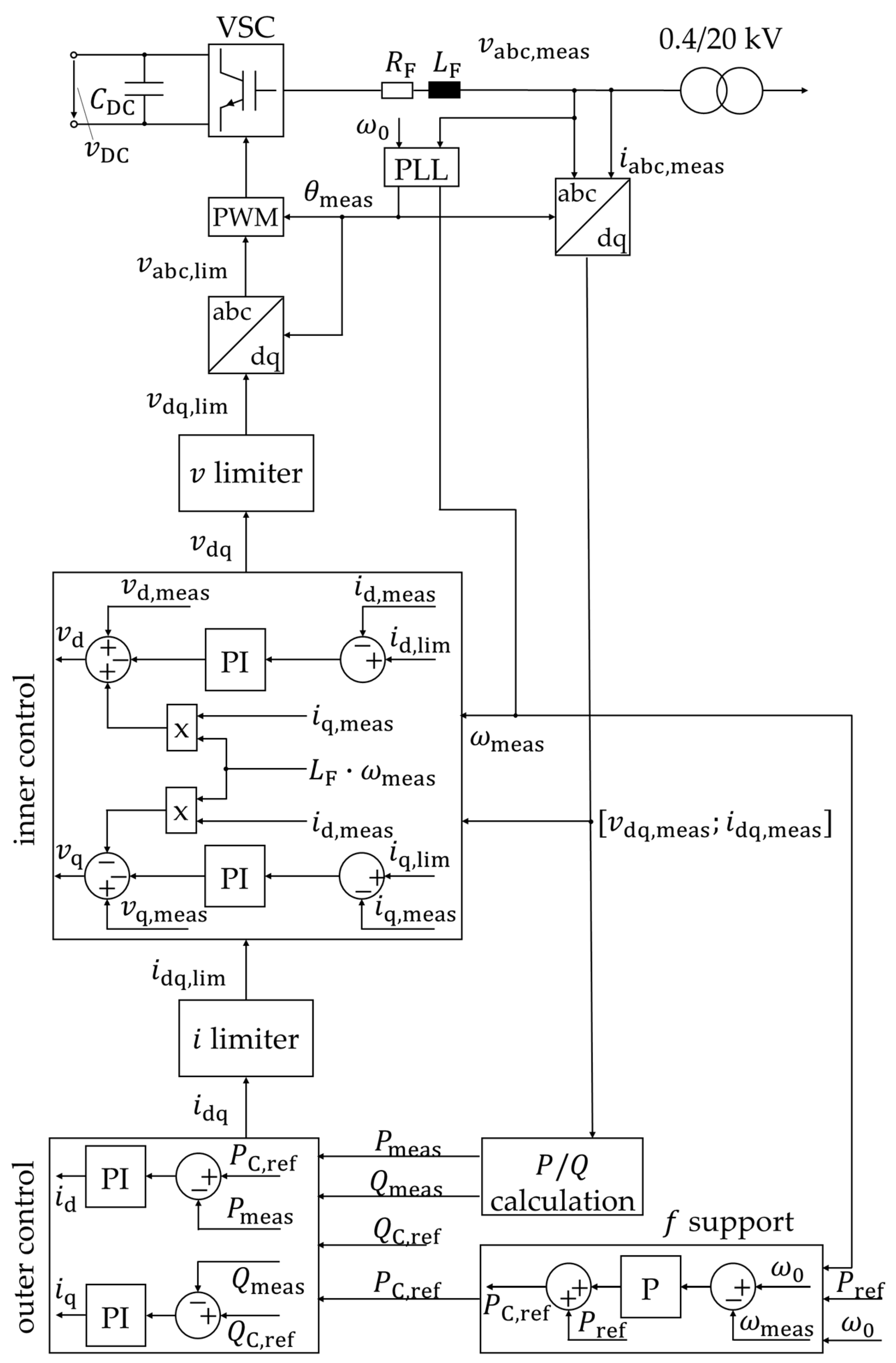
The RES is based on a full-size power VSC and modeled as an average value model with cascaded vector control and grid-supporting characteristics. It fulfills the German grid code requirements for voltage and frequency support. The electrical model is reduced to a controlled three-phase voltage source that is adjusted by the grid-supporting control. Only the grid-side converter and control are modeled under the assumption of a constant power infeed during the time interval of interest of a few seconds. The cascaded vector control of the VSC is implemented in a synchronous reference frame or direct and quadrature (dq) coordinates, as shown in Figure 9. 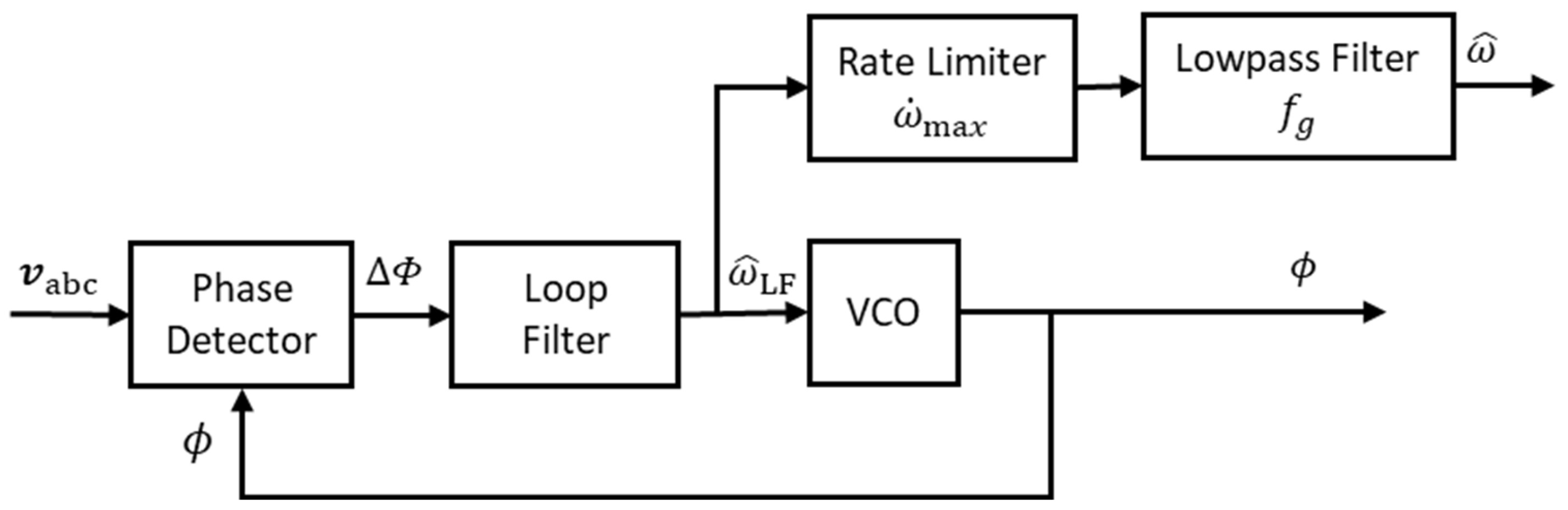The upper part of the figure shows the electrical model consisting of the VSC, the DC-side which is modeled as a constant voltage source and DC-link capacitor, the RES transformer and an RL-filter with the filter resistance R_F and the filter inductance L_F. The voltage and current measurements are implemented on the low-voltage side of the transformer. The control of the VSC relies on this local measurement. Since the grid-supporting control is implemented in dq coordinates, the frequency and angle estimation play major roles. Here, the PLL is depicted. However, in the context of this study, different frequency estimation methods are applied. The estimated angle derived from the voltage measurement is passed to the coordinate transformation blocks at the start and the end of the cascaded control.

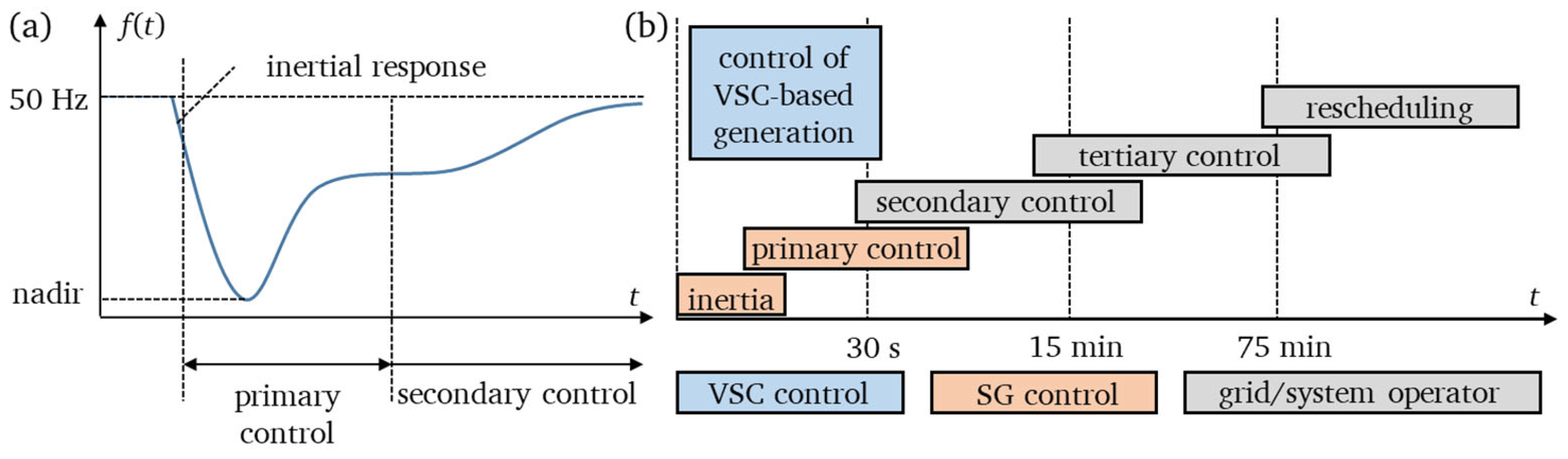
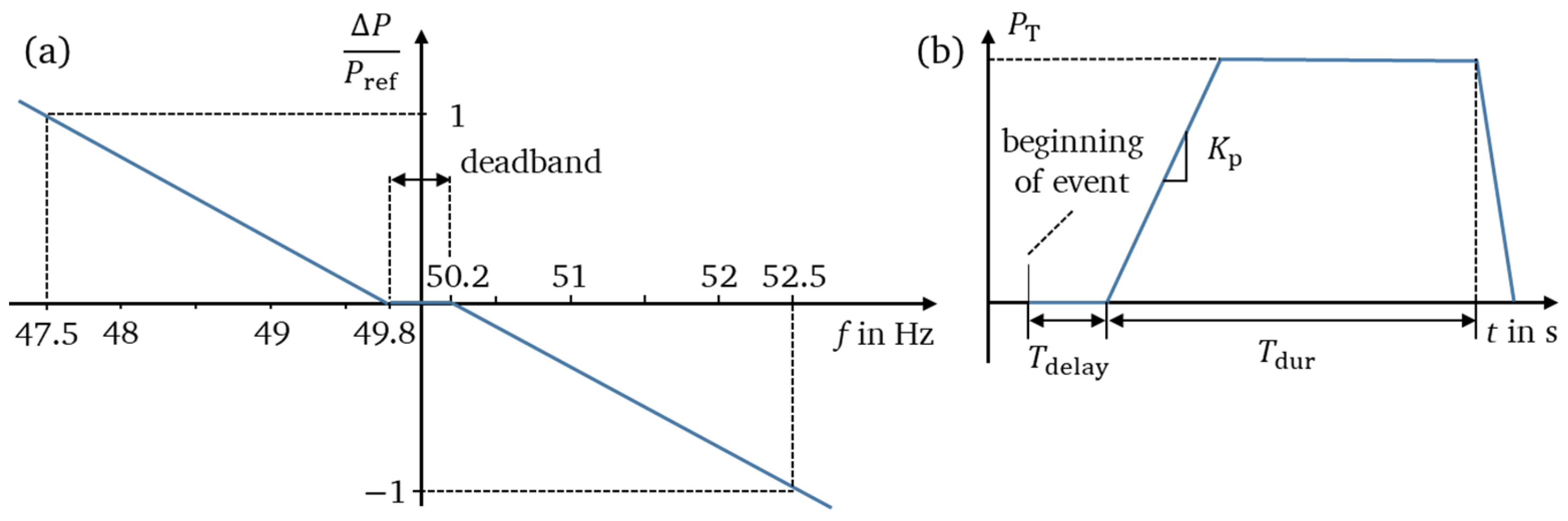
The three main blocks of the control are the frequency support, the outer control, and the inner control. The frequency support control implements the FFR with an active power-frequency droop P(f), as depicted in Figure 2a. Again, this serves as a placeholder and can also be implemented as the constant additional active power, as presented in Figure 2b. The high-level control or outer control is based on two proportional-integral (PI) controllers that compare the measured active and reactive power with the reference values. The output of the outer control is the reference values of direct and quadrature current i_d and i_q, which are passed to the inner control. The low-level control or inner control repeats a similar control for the current, leading to the reference values for direct and quadrature voltage. Additionally, the cross coupling in the inner current control takes into account that due to the filter inductance, the current lags the voltage, which must be considered in dq coordinates. Further details about cross-coupling control can be found, e.g., in [21]. Limiting the reference current output of the outer control includes the maximum overcurrent capacity of real converters to the model. Finally, the pulse width modulation (PWM) controls the individual switches of the converter. Since the average value model does not include a detailed converter model, the PWM is assumed to be ideal, and the controlled voltage output of the inner control is directly fed to the three-phase voltage source that represents the electrical model.

4.3. External Grid Model

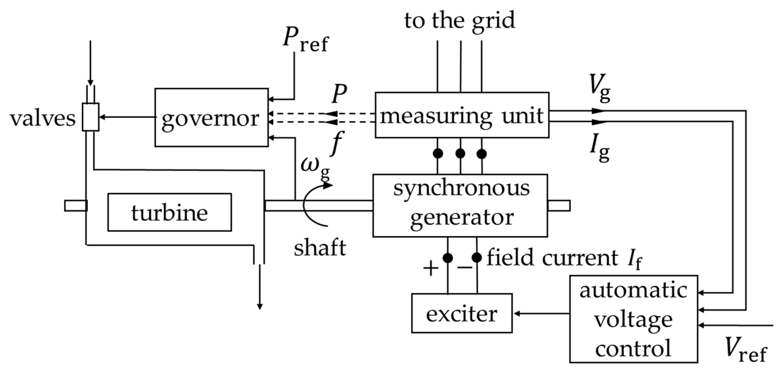
The external grid for dynamic frequency investigations is modeled as a sixth-order SG with a simplified governor, power system stabilizer (PSS), and excitation system. An overview of the synchronous generator control is given in Figure 10 and can be divided into the power-frequency control, which regulates the steam supply via valves, and the voltage and excitation control, which adjusts the field current. The machine and control parameters are adapted in order to replicate a frequency behavior of a low-inertia power system. The SG model is based on the synchronous machine’s subtransient and transient electromotive forces (emf), the corresponding time constants, and reactances.

The sixth-order SG model consists of four electrical and two mechanical states. The electrical states described in Equations (16)–(19) take into account the armature flux that gradually enters the rotor during a fault and, for this reason, affects the emf. The mechanical states given in Equations (20) and (21) describe the generator rotor swing. A detailed derivation of the equivalent circuit and the differential equations is given in [22]. The six differential equations describing the generator in a synchronous reference frame (SRF) are given in Equations (16)–(21).

$$T_{do}^{″}{\dot{E}}_q^{″}=E_q^{\prime }-E_q^{″}+I_d(X_d^{\prime }-X_d^{″})$$

(16)

$$T_{\mathrm{q}\mathrm{o}}^{″}{\dot{E}}_{\mathrm{d}}^{″}=E_{\mathrm{d}}^{\prime }-E_{\mathrm{d}}^{″}+I_{\mathrm{q}}(X_{\mathrm{q}}^{\prime }-X_{\mathrm{q}}^{″})$$

(17)

$$T_{\mathrm{d}\mathrm{o}}^{\prime }{\dot{E}}_{\mathrm{q}}^{\prime }=E_{\mathrm{f}}-E_{\mathrm{q}}^{\prime }+I_{\mathrm{d}}\left(X_{\mathrm{d}}-X_{\mathrm{d}}^{\prime }\right)$$

(18)

$$T_{\mathrm{q}\mathrm{o}}^{\prime }{\dot{E}}_{\mathrm{d}}^{\prime }=-E_{\mathrm{d}}^{\prime }+I_{\mathrm{q}}\left(X_{\mathrm{q}}-X_{\mathrm{q}}^{\prime }\right)$$

(19)

$$M·∆\dot{\omega }=P_{\mathrm{m},\mathrm{T}}-P_{\mathrm{e}} \mathrm{with} M=\frac{2·H·S_{\mathrm{r}}}{{\omega }_{\mathrm{r}}}$$

(20)

$$\dot{\delta }=∆\mathsf{\omega }={\omega }_{\mathrm{g}}-{\omega }_{\mathrm{r}}$$

(21)

$X_{\mathrm{d}}$, $X_{\mathrm{q}}$, $X_{\mathrm{d}}^{\prime }$, $X_{\mathrm{q}}^{\prime }$, $X_{\mathrm{d}}^{″}$, $X_{\mathrm{q}}^{″}$ are the synchronous, transient, and subtransient reactances in the d-axis and q-axis, $E_{\mathrm{f}}$, $E_{\mathrm{d}}^{\prime }$, $E_{\mathrm{q}}^{\prime }$, $E_{\mathrm{d}}^{″}$, $E_{\mathrm{q}}^{″}$ are the excitation emf, and the transient and subtransient emf in the d-axis and q-axis, respectively. $T_{\mathrm{d}\mathrm{o}}^{\prime }$,$T_{\mathrm{q}\mathrm{o}}^{\prime }$, $T_{\mathrm{d}\mathrm{o}}^{″}$, $T_{\mathrm{q}\mathrm{o}}^{″}$ are the d-axis and q-axis open-circuit transient and subtransient time constants and $I_{\mathrm{d}}$, $I_{\mathrm{q}}$ are the d-axis and q-axis component of the armature current. $M$, H, $∆\mathsf{\omega }$, $∆\dot{\mathsf{\omega }}$, ${\mathsf{\omega }}_{\mathrm{g}}$, ${\mathsf{\omega }}_{\mathrm{r}}$, $P_{\mathrm{m},\mathrm{T}}$, $P_{\mathrm{e}}$ and $\dot{\delta }$ are the angular momentum, the inertia constant, the rotor speed deviation and its derivation, the angular velocity of the generator, the rated synchronous angular velocity, the mechanical power of the turbine, the electromagnetic air-gap power, and the derivative of the rotor angle, respectively. The derivative quantities are derived with respect to time.

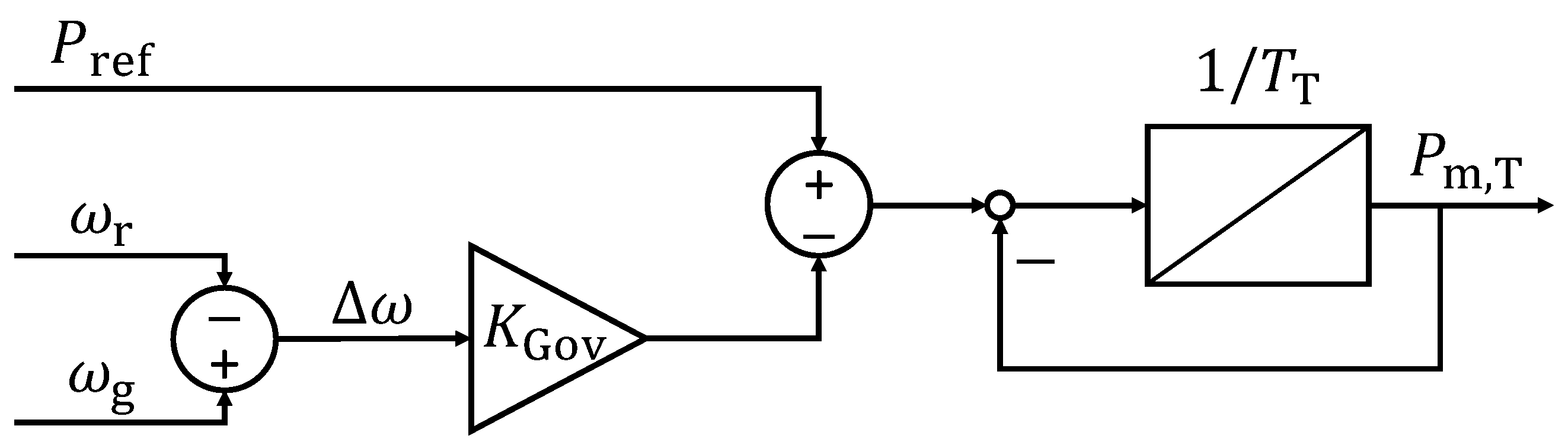
The SG, turbine, and automatic voltage control models are standard models of the Matlab/Simulink library with the parameters given in Appendix A. The focus of this study is on the governor since it mainly determines the frequency behavior of the generator. The governor control block is shown in Figure 11 and is based on [22]. P_ref, P_m,T, ω_r, and ω_g are the reference active power, the mechanical output power of the turbine, the rated frequency, and the measured grid frequency, respectively. K_Gov is the proportional gain of the frequency control and the inverse of the governor droop d_Gov. The turbine is considered as a time delay with the time constant T_T.

The parametrization of the SG and its control is based on a simple aggregation of multiple generation plants providing an inertial response to the system. The dynamics of the external grid are mainly defined by the installed power S_r of these plants, the inertia constant H, and the governor droop d_Gov. According to the coherency method, the SG of the overlying high-voltage grid is assumed to be coherent. Therefore, the aggregate model parameters can be derived from Equations (22)–(24). Assuming that in future scenarios, not all of the power plants can provide an inertial response, the aggregate parameters are related to the total system load P_L.

The aggregate governor droop d_Gov,agg and the aggregate inertia constant H_agg are both calculated by the sum of the weighted values for each generator and referred to the total load of the system as shown in Equations (22) and (23). The installed power of the aggregate generator S_r,agg is calculated using Equation (24). It takes into account the aggregate short-circuit power S_SC and the R to X ratio of the corresponding system. The subtransient d-axis reactance $x_{\mathrm{d}}^{″}$ is given in p.u. and the maximum voltage factor is assumed to be $c_{\mathrm{m}\mathrm{a}\mathrm{x}}=1.1$.

$$d_{\mathrm{G}\mathrm{o}\mathrm{v},\mathrm{a}\mathrm{g}\mathrm{g}}=\frac{P_{\mathrm{L}}}{{\sum }_{i=1}^{N_{\mathrm{G}}}{K}_{\mathrm{G}\mathrm{o}\mathrm{v},i}·P_{\mathrm{r}\mathrm{G},i}}$$

(22)

$$H_{\mathrm{a}\mathrm{g}\mathrm{g}}=\frac{{\sum }_{i=1}^{N_{\mathrm{G}}}{H}_i{·S}_{\mathrm{r}\mathrm{G},i}}{P_{\mathrm{L}}}$$

(23)

$$S_{\mathrm{r},\mathrm{a}\mathrm{g}\mathrm{g}}=x_{\mathrm{d}}^{″}\sqrt{{1+\left(\frac{R}{X}\right)}^2}\frac{S_{\mathrm{S}\mathrm{C}}}{c_{\mathrm{m}\mathrm{a}\mathrm{x}}}$$

(24)

The total load active power P_L is used for the calculation to take into account that not all generating plants provide inertial behavior.$N_{\mathrm{G}}$, $H_i,K_{\mathrm{G}\mathrm{o}\mathrm{v},i}$, $P_{\mathrm{r}\mathrm{G},i}$,$S_{\mathrm{r}\mathrm{G},i}$ are the number of SGs in the overlying grid as well as the inertia constant, the governor gain, the installed active, and the apparent power of the i-th generator. For the parameter derivation, typical machine parameters and power system characteristics are used based on [1,5,22,23]. The aggregate parameters are given in

Table 2. Aggregated parameters for the overlying grid.

Parameter	Symbol	Value
Governor droop	$d_{\mathrm{G}\mathrm{o}\mathrm{v},\mathrm{a}\mathrm{g}\mathrm{g}}$	5%
Inertia constant	$H_{\mathrm{a}\mathrm{g}\mathrm{g}}$	5 s
Rated power	$S_{\mathrm{r},\mathrm{a}\mathrm{g}\mathrm{g}}$	30.8 MVA
Turbine time constant	$T_{\mathrm{T}}$	0.3 s
Onsite power load	$S_{\mathrm{r},\mathrm{o}\mathrm{n}\mathrm{s}\mathrm{i}\mathrm{t}\mathrm{e}}$	3.08 MVA

. The detailed model parameters are given in Appendix A. The onsite load of the aggregated SG is assumed to be 10% of the installed power. In the following sections, the index agg is replaced by SG in order to name the components according to Figure 8.

5. Evaluation Criteria

Uniform criteria must be defined for a qualitative evaluation and comparison of the frequency estimation results. As described in Section 2.2, the primary control is activated if the frequency in the power system deviates from the nominal frequency by more than ±10 mHz. For deviations of more than ±200 mHz, additional safety mechanisms are triggered. To avoid false triggering of these mechanisms, it is important that the signal is estimated as accurately as possible and that the maximum deviation remains small. The German Grid Code VDE-AR-N-4110 [24] specifies a maximum frequency deviation in the steady state of ±10 mHz. In the case of rapid frequency changes, the minimum accuracy should be ±50 mHz. Starting from this motivation, three criteria are defined according to which the results of the estimation methods are evaluated. One main criterion is defined, which is the aim of tuning from the parameters. The secondary and tertiary criteria are used to evaluate and describe the estimation result. The criteria are:

• Main criterion: A large deviation of the estimated value from the real measured frequency can have far-reaching consequences for the power system. For this reason, the aim of the estimation methods is to achieve the lowest possible maximum deviation according to Equation (25).

$${\mathsf{\Delta }}_{\mathrm{m}\mathrm{a}\mathrm{x}}=\max \left|\widehat{f}\left(t\right)-f_{\mathrm{S}\mathrm{G}}(t)\right|$$

(25)

Here, $\widehat{f}\left(t\right)$ is the estimated frequency and $f_{\mathrm{S}\mathrm{G}}\left(t\right)$ is the frequency of the synchronous generator as the reference value.

2.

Secondary criterion: The frequency curves of two estimation methods with the same maximum deviation can turn out very differently. For this reason, the error area according to Equation (26), is evaluated over the period of simulation.

$${\Delta }_{\mathrm{A}}={\int }_0^{1.5\mathrm{s}}\left|\widehat{f}\left(t\right)-f_{\mathrm{S}\mathrm{G}}(t)\right|\mathrm{d}t$$

(26)

3.

Tertiary criterion: Since the frequency curve serves as the input parameter for the inverter control, it makes sense that it has a smooth curve. As a criterion, it qualitatively evaluates how smooth the estimated frequency curve is.

For evaluation of the FFR control, the active power infeed of the RES, according to Figure 2, is evaluated. Additionally, Equations (27) and (28) determine the RoCoF as defined in Section 2.2 as well as the frequency nadir. The RoCoF is calculated over a time window of 500 ms in accordance with [25,26]. The frequency nadir indicates the absolute minimum of the frequency curve.

$$RoCoF=\frac{\mathrm{d}f\left(t\right)}{\mathrm{d}t}=\frac{f\left(t=500 \mathrm{m}\mathrm{s}\right)-f\left(t=0 \mathrm{s}\right)}{500 \mathrm{m}\mathrm{s}}$$

(27)

$$f_{\mathrm{n}\mathrm{a}\mathrm{d}\mathrm{i}\mathrm{r}}=\mathrm{m}\mathrm{i}\mathrm{n}f\left(t\right)$$

(28)

6. Results

This section presents the simulation results for the frequency estimation methods, the sensitivity analysis, and the linearization of sensitive parameters. Finally, the linearized parametrization for the frequency estimation methods is applied as an input to the converter control. Figure 12 compares the frequency curve measured at the PCC of the medium-voltage testbench with the PLL standard parametrization to the rotational speed of the SG. The limits of the standard PLL become clearly visible. While the steady states before and shortly after the load step are well met, the transient time range shows large oscillations reflecting the electrical transients occurring in EMT simulations. These transient oscillations are mainly defined by the rate limiter, whereas in the SG model, the rotational speed is a state variable and therefore less susceptible to transients.

6.1. Comparison of Frequency Estimation Methods

In this section, simulations are carried out with the model and the reference case described in Section 4. The parameters of the frequency estimation methods are tuned. For this purpose, the influencing factors of the individual methods are identified and adjusted in such a way that optimal estimation results are achieved with regard to the defined evaluation criteria.

The results of the offline frequency estimation methods Gauss–Newton, Zero-Crossing, and recursive Gauss–Newton are presented in Figure 13. Here, the temporal course of the deviation from the SG frequency is shown for the methods. With the GN method, a smooth course with few fluctuations is achieved, but with the largest maximum deviation compared to the other methods (blue curve). For the RGN method, the deviation fluctuates up to a time of approximately t = 1 s so a smooth course of the frequency estimation is only achieved afterward (yellow curve). Additionally, high-frequency oscillations with small amplitude occur for the RGN method, which cannot be seen in Figure 13. The small oscillations can be eliminated by stronger filtering, but this leads to a larger maximum deviation. The ZC method achieves the smallest maximum deviation at the time $t\approx 0.6 \mathrm{s}$ and a smooth curve from $t\approx 0.25 \mathrm{s}$ onwards (red curve). The transient response to the new stationary frequency is also faster here than with the other methods. Due to these findings, the ZC method is considered the best result in offline estimation.

Figure 14 shows the results of the frequency estimation using online or real-time methods. The RGN method achieves a frequency response with a small maximum deviation, but a high-frequency oscillation occurs starting at time $t=0.25 \mathrm{s}$. This can be reduced by stronger filtering, which, however, also reduces the quality of the estimate. The ZC method has the largest deviations but with a very smooth course (red curve). The frequency estimation using a PLL achieves results with the smallest maximum deviation and a smooth course (blue curve). The transient response of the PLL to the new stationary frequency is faster than with the other methods.

Table 3. Tuned parameters for best frequency estimation when applying a load step of $\mathsf{\Delta }{P}_{\mathrm{L}\mathrm{o}\mathrm{a}\mathrm{d}}=3 \mathrm{M}\mathrm{V}\mathrm{A}$. Underlined parameters are sensitive to tuning.

	Method	Parameter	Value
online	PLL	Rate limit	0.85 Hz·s−1
		Filter frequency fg	25 Hz
		PID controller kp, ki, kd	30, 1 s, 0.04 s−1
	ZC	Rate limit	0.75 Hz·s−1
		Filter frequency fg	25 Hz
	RGN	Initial covariance matrix P0	104 E
		Memory factor ${\lambda }_k$	0.9
		Rate limit	0.8 Hz·s−1
		Filter frequency fg	20 Hz
offline	GN	Maximum iteration maxit	50
		Accuracy $\epsilon$	10−30
		Window width m	40 samples
		Rate limit	0.75 Hz·s−1
		Moving average filter	120 samples
	ZC	Rate limit	1.9 Hz·s−1
		Moving average filter	8 samples
	RGN	Initial covariance matrix P0	104 E
		Memory factor ${\lambda }_k$	0.86
		Rate limit	0.72 Hz·s−1
		Moving average filter	20 samples

presents the tuned parameters for all methods. Sensitive parameters, i.e., parameters that have an impact on the quality of the frequency estimation, are underlined in Table 3.

By comparing all methods, the online frequency estimation using a PLL achieves the best results, but tuning the parameters is the most time-consuming for this method as it has the largest number of sensitive parameters, cf. Table 3. The results of the RGN method show oscillations. By stronger filtering, the resulting absolute deviation increases and the results of this method turn out even worse. The largest deviations are achieved by the ZC method, but in turn, this method has a smooth frequency curve and a simple setting of the parameters. With only two sensitive parameters for the tuning of the method, sufficiently small deviations during transients and a smooth curve, the ZC method is considered the most promising here.

Table 4. Comparison of best frequency estimation results according to evaluation criteria.

	Method	Δmax in mHz 1	ΔA in mHz·s 2	Smooth Curve
Online	PLL	8.384	6.163	Yes
	ZC	13.360	9.540	Yes
	RGN	11.560	7.516	No
Offline	GN	12.220	8.940	Yes
	ZC	10.690	7.160	Yes
	RGN	11.720	8.363	No

¹ Maximum deviation from synchronous generator frequency. ² Area error between estimated frequency and synchronous generator frequency curve.

shows the results for the tuning of the frequency estimation methods according to the three evaluation criteria defined in Section 5. Overall, all methods estimate the frequency of the SG well, not exceeding a maximum deviation with the online ZC method of ${\mathsf{\Delta }}_{\mathrm{m}\mathrm{a}\mathrm{x}}=13.360 \mathrm{m}\mathrm{H}\mathrm{z}$. The PLL achieves the best results for the maximum deviation as well as for the area error. By all methods, an accuracy of ${\mathsf{\Delta }}_{\mathrm{m}\mathrm{a}\mathrm{x}}<50 \mathrm{m}\mathrm{H}\mathrm{z}$ is achieved, as required in [13] for the transient range.

6.2. Linearization of Relevant Parameters

In the following, the robustness of the estimation methods to the change of input variables is investigated. For this purpose, the testbench shown in Figure 8 is subjected to a variable load step of $\mathsf{\Delta }{P}_{\mathrm{L}}=2\dots 5 \mathrm{M}\mathrm{W}$, and the estimation of how the algorithms behave is tested. Figure 15 shows the frequency estimation using a PLL with the tuned parameters according to Table 3 for different load steps. Here, the PLL provides optimal results for a load step of $\mathsf{\Delta }{P}_{\mathrm{L}}=3 \mathrm{M}\mathrm{W}$ as the parameters are tuned for this case. The results show that by changing the magnitude of the load step and keeping the parameters constant, the quality of the results of the estimation procedure decreases drastically during the transients. This can be explained by the settings of the rate limiter that prevent the frequency estimation from matching the steeper curves.

For the three online methods PLL, RGN, and ZC, the parameters are now set in such a way that for each load step, individually, the deviation of the estimated frequency from the generator frequency as well as the error area of the two frequency curves are minimized. These tuned parameters are shown in Figure 15. The number of sensitive parameters that have an influence on the quality of the frequency estimation is three for the PLL and two for the ZC and RGN methods each. These parameters are the rate limit (RL) of the rate limiter and the cut-off frequency of the low-pass filter f_g for the ZC and the RGN method, and additionally, the proportional factor $k_{\mathrm{p}}$ of the PID controller of the PLL. Figure 16 shows that the sensitive parameters of the methods show a linear relationship with the magnitude of the load step. The ZC method shows the best robustness to changes in the size of the load step, in particular, simulations show that the quality of the estimate is largely independent of the parameters of the method. However, there are only a few degrees of freedom in the tuning for this method, so the PLL provides better results in the tuning for a special design case.

From the tuned parameters, according to Figure 16, the following dependencies are calculated and implemented in the simulations:

$$\mathrm{R}\mathrm{L}=\left\{\begin{array}{c}0.12 \mathrm{H}\mathrm{z}/\mathrm{s}+0.22 \mathrm{H}\mathrm{z}/\mathrm{s}·\mathsf{\Delta }{P}_{\mathrm{L}}/\mathrm{M}\mathrm{V}\mathrm{A} \mathrm{f}\mathrm{o}\mathrm{r} \mathrm{P}\mathrm{L}\mathrm{L}\\ 0.12 \mathrm{H}\mathrm{z}/\mathrm{s}+0.22 \mathrm{H}\mathrm{z}/\mathrm{s}·\mathsf{\Delta }{P}_{\mathrm{L}}/\mathrm{M}\mathrm{V}\mathrm{A} \mathrm{f}\mathrm{o}\mathrm{r} \mathrm{Z}\mathrm{C}\\ 0.12 \mathrm{H}\mathrm{z}/\mathrm{s}+0.22 \mathrm{H}\mathrm{z}/\mathrm{s}·\mathsf{\Delta }{P}_{\mathrm{L}}/\mathrm{M}\mathrm{V}\mathrm{A} \mathrm{f}\mathrm{o}\mathrm{r} \mathrm{R}\mathrm{G}\mathrm{N}\end{array}\right.$$

(29)

$$f_g=\left\{\begin{array}{c}0.74 \mathrm{H}\mathrm{z}+10.0 \mathrm{H}\mathrm{z}·\mathsf{\Delta }{P}_{\mathrm{L}}/\mathrm{M}\mathrm{V}\mathrm{A} \mathrm{f}\mathrm{o}\mathrm{r} \mathrm{P}\mathrm{L}\mathrm{L}\\ 9.20 \mathrm{H}\mathrm{z}+5.15 \mathrm{H}\mathrm{z}·\mathsf{\Delta }{P}_{\mathrm{L}}/\mathrm{M}\mathrm{V}\mathrm{A} \mathrm{f}\mathrm{o}\mathrm{r} \mathrm{Z}\mathrm{C}\\ 14 \mathrm{H}\mathrm{z}·\mathsf{\Delta }{P}_{\mathrm{L}}/\mathrm{M}\mathrm{V}\mathrm{A} \mathrm{f}\mathrm{o}\mathrm{r} \mathrm{R}\mathrm{G}\mathrm{N}\end{array}\right.$$

(30)

$$k_{\mathrm{p}}=6.26+7.24·\mathsf{\Delta }{P}_{\mathrm{L}}/\mathrm{M}\mathrm{V}\mathrm{A} \mathrm{f}\mathrm{o}\mathrm{r} \mathrm{P}\mathrm{L}\mathrm{L}$$

(31)

The rate limit RL, as well as the low-pass filter cut-off frequency $f_g$ are quantities that modify the estimated frequency following the individual methods and have the main impact on the quality of the results. Here, the electrical transients in the system are tried to be eliminated. It is noticeable that the rate limit in Equation (29) is identical for the three methods. The interpolated dependency of the filter cut-off frequency f_g for the RGN method is corrected from the interpolation result in such a way that a negative offset is eliminated in order to cope with the physical limits.

Figure 17 shows the frequency estimation results with linearized parameters according to Equations (29)–(31) at the PCC of the medium-voltage testbench. For all three online methods, the results show a good estimation of the SG frequency, elimination of the transient oscillations, and a good fit of the RoCoF.

6.3. Fast-Frequency Response with Optimized Local Frequency Estimation

This section implements the linearized parametrization of the online frequency estimation methods to the input of the FFR control of the VSC-based RES. The frequency estimation is applied to the FFR control block only; the phase angle estimation is still done by means of a PLL with standard parametrization. For comparison, the SG speed and the PLL with standard parametrization are presented in order to classify the results.

Table 5. Comparison of Rate of Change of Frequency (RoCoF) and frequency nadir $f_{\mathrm{m}\mathrm{i}\mathrm{n}}$ for the different scenarios with linearized parametrization as input for the fast frequency response (FFR).

		Linear FFR		Constant FFR
Load Step	Method	RoCoF in Hz/s	fmin in Hz	RoCoF in Hz/s	fmin in Hz
$\mathsf{\Delta }{P}_{\mathrm{L}}=2 \mathrm{M}\mathrm{W}$	PLL	0.4434	49.4790	0.4628	49.4569
	ZC	0.4738	49.4796	0.4900	49.4576
	RGN	0.4673	49.4797	0.4791	49.4577
	SG	0.4770	49.4797	0.4894	49.4579
$\mathsf{\Delta }{P}_{\mathrm{L}}=3 \mathrm{M}\mathrm{W}$	PLL	0.6679	49.2195	0.6979	49.1928
	ZC	0.6952	49.2199	0.7159	49.1933
	RGN	0.6876	49.2201	0.7189	49.1935
	SG	0.7023	49.2200	0.7283	49.1935
$\mathsf{\Delta }{P}_{\mathrm{L}}=4 \mathrm{M}\mathrm{W}$	PLL	0.8771	48.9692	0.9113	48.9391
	ZC	0.9003	48.9695	0.9162	48.9394
	RGN	0.8908	48.9697	0.9255	48.9396
	SG	0.9127	48.9695	0.9443	48.9395
$\mathsf{\Delta }{P}_{\mathrm{L}}=5 \mathrm{M}\mathrm{W}$	PLL	1.0680	48.7286	1.0943	48.6968
	ZC	1.0864	48.7289	1.0795	48.6970
	RGN	1.0750	48.7291	1.0952	48.6973
	SG	1.1041	48.7288	1.1357	48.6970

shows the RoCoF and nadir evaluation for different load steps and compares the results for the linear FFR and the constant power output FFR. The RoCoF and nadir of the frequency curves for each estimation method and load step are calculated according to Equations (3) and (4). The results in Table 5 show that the PLL leads to the largest RoCoF deviations from the SG values, while the ZC achieves the overall best fit. The frequency nadir $f_{\mathrm{m}\mathrm{i}\mathrm{n}}$ is well met by all methods. This is because the transient differences are only relevant in the first 100 ms after the disturbances, cf. Figure 12. The difference between the two implementations of FFR, according to Figure 2, show that the linear FFR has a stronger impact on the frequency than the constant FFR. Due to the deadband of only 50 mHz, the linear FFR starts adapting the output power earlier so that the constant FFR is triggered at a frequency deviation of 200 mHz.

Figure 18 shows the active power response of the VSC-based RES after a load step using different frequency estimation inputs for the linear FFR according to Figure 2a. The curves of different frequency estimation methods are similar and show the increase in the active power output proportional to the estimated frequency deviation after the deadband of 50 mHz is reached at $t=0.125 \mathrm{s}$. When using the SG speed as input for the FFR control, the curve is smoothest, while the standard PLL parametrization according to Appendix B leads to oscillations in the active power infeed, as can be seen in the enlarged area between 0.1 s and 0.18 s shown within Figure 18. The linearized frequency estimation methods PLL, ZC, and RGN do not show significant oscillations but lead to a small time delay of the active power infeed, which is largest for the linearized PLL method. In conclusion, the linearized parametrization of the frequency estimation methods improves the FFR by smoothening the active power output and reducing transient oscillations.

7. Conclusions

Frequency estimation in the power system requires the use of real-time capable or online methods, where the measurement and evaluation of the frequency are done in real time. After a disturbance in the system, transient compensation processes are caused. The transient frequency, i.e., the frequency in the short-term range after a disturbance before a new quasi-stationary state is reached, can be estimated indirectly from a voltage measurement by various methods. The already widely used solution of Phase-Locked-Loops provides satisfactory results after tuning the relevant parameters. The two additional methods Zero-Crossing and recursive Gauss–Newton can also fulfill the accuracies specified by the German Grid Code. However, deviations remain between the estimated frequencies and the mechanical frequency or rotational speed of a synchronous generator, which is used for comparison. In particular, the filters and limiters used can be tuned for individual reference cases.

In the first step, different methods for online and offline estimation of the grid frequency are implemented and compared. The offline methods, namely the Zero-Crossing, Gauss–Newton, and recursive Gauss–Newton methods, are evaluated after finishing the simulation. The online methods Phase-Locked Loop, Zero-Crossing, and recursive Gauss–Newton method are implemented in the simulation. All methods reach a maximum deviation of 14 mHz compared to the rotor speed of the synchronous generator and are thus very well within the required tolerance band of ±50 mHz during transients. Regarding the maximum deviation and the error area, the tuned Phase-Locked Loop provides the best frequency estimate. The investigations of the robustness of the methods show that there is a linear relationship between the sensitive parameters and the magnitude of the load step. With only two sensitive parameters, the Zero-Crossing method is the most robust.

Based on the tuned parameters, a linear correlation is found between the sensitive parameters of the frequency estimation methods and the size of the load step applied to the system. These linearized parameters can be applied in simulations and lead to improved results of the frequency estimation. In the final step, these real-time frequency estimates are passed to the fast frequency control of a converter-based renewable energy source. The active power output of the converter as a response to the frequency drop is improved and approaches the response that can be achieved by using the synchronous generator speed as an input to the control.

For the simulation of power systems, the results offer the possibility of robust, accurate, and communication-free estimation of the frequency during transients. Thus, even in simulations without rotating resources, the frequency can be reliably evaluated. In the real system, on the other hand, the event or disturbance is not known, so the results show a theoretical approach for application in power system simulations or a real-time dynamic state estimation is required. Future research can be conducted by adapting the sensitive parameters for other sensitivities, e.g., the power system inertia, and by testing the theoretical results in an experimental setup for application in real power systems. Further investigations with the presented parameters can be conducted in power systems with a larger share of converter-based generation plants.