Air Pollution Monitoring via Wireless Sensor Networks: The Investigation and Correction of the Aging Behavior of Electrochemical Gaseous Pollutant Sensors

Abstract

The continuously growing human activity in large and densely populated cities pollutes air and consequently puts public health in danger. This is why air quality monitoring is necessary in all urban environments. However, the creation of dense air monitoring networks is extremely costly because it requires the usage of a great number of air monitoring stations that are quite expensive. Instead, the usage of wireless sensor networks (WSNs) that incorporate low-cost electrochemical gas sensors provides an excellent alternative. Actually, sensors of this kind that are recommended for low-cost air quality monitoring applications may provide relatively precise measurements. However, the reliability of such sensors during their operational life is questionable. The research work presented in this article not only experimentally examined the correlation that exists between the validity of the measurements obtained from low-cost gas sensors and their aging, but also proposes novel corrective formulae for gas sensors of two different types (i.e., NO₂, O₃), which are aimed at alleviating the impact of aging on the accuracy of measurements. The following steps were conducted in order to both study and lessen the aging of electrochemical sensors: (i) a sensor network was developed to measure air quality at a place near official instruments that perform corresponding measurements; (ii) the collected data were compared to the corresponding recordings of the official instruments; (iii) calibration and compensation were performed using the electrochemical sensor vendor instructions; (iv) the divergence between the datasets was studied for various periods of time and the impact of aging was studied; (v) the compensation process was re-evaluated and new compensation coefficients were produced for all periods; (vi) the new compensation coefficients were used to shape formulae that automatically calculate the new coefficients with respect to the sensors’ aging; and (vii) the performance of the overall procedure was evaluated through the comparison of the final outcomes with real data.

1. Introduction

Continuous advances achieved in the technology of microelectromechanical systems (MEMS) have made it feasible to mass-produce inexpensive devices that, despite their small dimensions, have enhanced capabilities of sensing, processing, and communicating [1]. The wireless interconnection of several devices of this type, referred to as sensor nodes, gave birth to wireless sensor networks (WSNs) [2]. The architecture of a WSN is illustrated in Figure 1. A typical sensor node comprises a processing unit, one or more sensors, a transceiver, and a power unit, which in most cases is a battery. WSNs, by taking advantage of the collaborative use of their sensor nodes, are able to not only monitor the ambient conditions over wide areas of interest but also process sensed data and wirelessly transmit them over long distances, via gateways referred to as base stations [3]. For this reason, although their operation is hampered by problems of various kinds such as connectivity loss, congestion, vulnerable security, inadequate coverage, and most of all by the extremely restricted energy adequacy of their sensor nodes [4,5,6,7,8,9,10,11,12], WSNs have the potential to support almost any field of human activity and therefore have an ever-increasing range of applications [13,14,15,16,17]. The monitoring of air quality is not only one of the numerous applications of WSNs but also an absolutely fundamental operation performed by the use of the Internet of Things (IoT) [18] in so-called “smart cities”, where urban operations are performed efficiently with minimum human intervention [19,20].

Indeed, there is no doubt that air pollution is among the greatest threats against public health. This is why air quality monitoring is necessary in all populated areas. However, in wide urban areas this operation is extremely costly because it requires the creation of dense monitoring networks comprising expensive scientific stations [21,22]. On the other hand, a grid network of densely installed low-cost air quality monitoring devices can also provide detailed information on the ambient air quality. Actually, the production of low-cost devices for gas pollutant sensing is feasible thanks to recent technological advances. At the same time, various research works have tried to optimize the effectiveness of such sensors by applying techniques such as machine learning and other artificial intelligence tools [23,24,25,26,27,28]. In this way, the development and installation of low-cost air quality sensors has become increasingly important [29] as a partial solution to the problem of supplementary coverage of an area. Actually, devices of this kind do not aim at replacing corresponding scientific instruments of high accuracy, but rather at being an additional source of air quality information, provided that their results are reliable [30]. This is why the development of such sensing devices has been investigated in several research works [31,32,33,34,35,36,37,38].

The research work that is presented in this article experimentally evaluated the reduction in measurement accuracy of low-cost gas pollutant electrochemical sensors because of their aging and proposes corresponding corrective formulas. In what follows, in Section 2, the relative theoretical background is established. In Section 3, both the infrastructure is established and the procedures followed in the experiments performed are described. In Section 4, the results of the experiments carried out are both presented and discussed and the formulae proposed for corrective use are described and experimentally evaluated. Finally, in Section 5, concluding remarks are drawn.

2. Theoretical Background

Nowadays, there are many different types of low-cost gaseous pollutant sensors that are commercially available [39]. The most commonly used types are the electrochemical sensors because they are able to detect and measure the concentrations of various gases with a relatively high sensitivity and short response time [40].

Typically, the monitoring of pollutant gases in urban areas by using electrochemical sensors requires the ability to sense lower concentrations of gases than those existing in industrial areas [41]. The detection and analysis of low concentrations necessitates the usage of models that take into consideration the impact of exogenous factors such as temperature, humidity, and pressure, which affect the operation of the electrodes of electrochemical sensors [42], so that the measured values are accurate. Practically, the output of an electrochemical sensor is an electric current of the order of μA, which is then converted to voltage that is analogous to the concentration of the gas detected.

However, various research studies have demonstrated that the measurements made by low-cost air quality sensors have, in many cases, low reliability compared to the measurements made by using reference monitoring instruments [40,43,44,45,46,47]. Specifically, these studies showed that the accuracy of such sensors is influenced by not only exogenous factors related to environmental conditions, such as air temperature, relative humidity, and interferences with other gases (cross-sensitivity), but also endogenous factors of the sensors such as warming-up time, gain, and initial manufacturer calibration [48,49].

Also, many research studies have been conducted regarding the evaluation of low-cost air quality sensors. Actually, there are two methods with which to study and evaluate the performance of low-cost gas sensors. The first method is to evaluate the gas sensors in a laboratory environment, i.e., under controlled conditions [45,50,51,52,53,54,55]. The second method proposes the evaluation of gas sensors in the field with nearby reference measuring instruments, so that low-cost sensors are calibrated by comparing the measured data that they produce with the data obtained from reference instruments [56,57,58,59,60]. The second method seems to lead to more accurate and reliable results, because the environmental parameters such as temperature and humidity are taken into consideration, contrary to what happens in the corresponding procedure that is conducted in laboratory environments. Linear regression (LR), multiple linear regression (MLR) and machine learning models are the most widely used methods to calibrate low-cost sensors [61,62]. In addition, a learning systems-based generative adversarial network (GAN) research team [63] proposed a GAN-based automatic property generation (GAPG) approach to generate verification properties supporting model checking. Conversely, the time-series feature of the IoT makes the data density and the data dimension higher; as such, anomaly detection is important to ensure hardware and software security, and research work [64] has proposed a memory-augmented encoder approach to detect anomalies in IoT data, which aims to use reconstruction errors to determine data anomalies. While the aging of electrochemical sensors is a given problem, the treatment of measurements during aging remains on the table. Based on this, the investigation of equations that include correction factors to compensate and improve the measurements during their lifetime was the subject of research of this work.

Regarding the electrochemical gas sensors, their operation is based on the chemical reactions performed between environmental air and electrodes that are within a liquid vessel that is incorporated inside the sensor units [65]. The creation of dense air monitoring networks is both more affordable and easier to be deployed by using low-cost electrochemical sensors rather than high-cost monitoring instruments. On the other hand, when using low-cost electrochemical sensors, not only is the calibration of the sensors affected by ambient conditions in external environments but also sensors must be replaced at 1–2-year intervals due to the rapid wear of their chemical elements [66].

Actually, the aging of the sensors and the accuracy of their response during their lifetime have not been sufficiently studied. Research works have shown that aging biases the voltage recording at certain environmental O₃ concentrations (approximately 20% after 9 months of continuous operation), thus necessitating frequent calibration of the oxidizing gas sensor [67]. It has also been demonstrated that the deterioration of sensors due to aging is a non-reversible process. Specifically, it has been found that over long deployments (>2 years), the sensor likely becomes insensitive to NO₂ and O₃. Therefore, the prompt identification and replacement of nonfunctional sensors is essential in order to ensure reliable data acquisition in long-term field deployments [68]. The investigation of aging correction factors of low-cost electrochemical sensors were part of this work, as well as how well the use of aging correction models can realistically reproduce measurements during their lifetime.

3. Analysis of the Experimental System and Procedure

As aforementioned, the research work presented in this article not only studies the deterioration that is caused due to aging in the performance of low-cost sensors that are used for air monitoring in smart cities, but also introduces a method that aims at maintaining high levels of accuracy despite the aging of sensors. For this reason, a WSN comprising low-cost electrochemical sensors [69] was developed by the authors of this article to monitor the concentrations of nitrogen dioxide (NO₂) and ozone (O₃) in the ambient air, Then, in the long run (i.e., 3 months, 6 months, and 8 months) the performance of the low-cost sensors was compared with the reference instruments and was re-evaluated. In what follows in Section 3, the experimental system developed and the initial procedures followed for the calibration of the sensors are described.

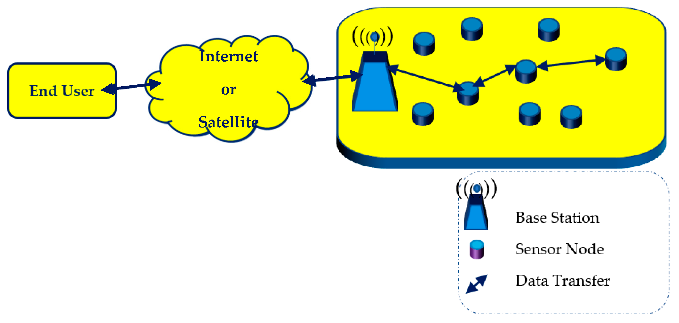
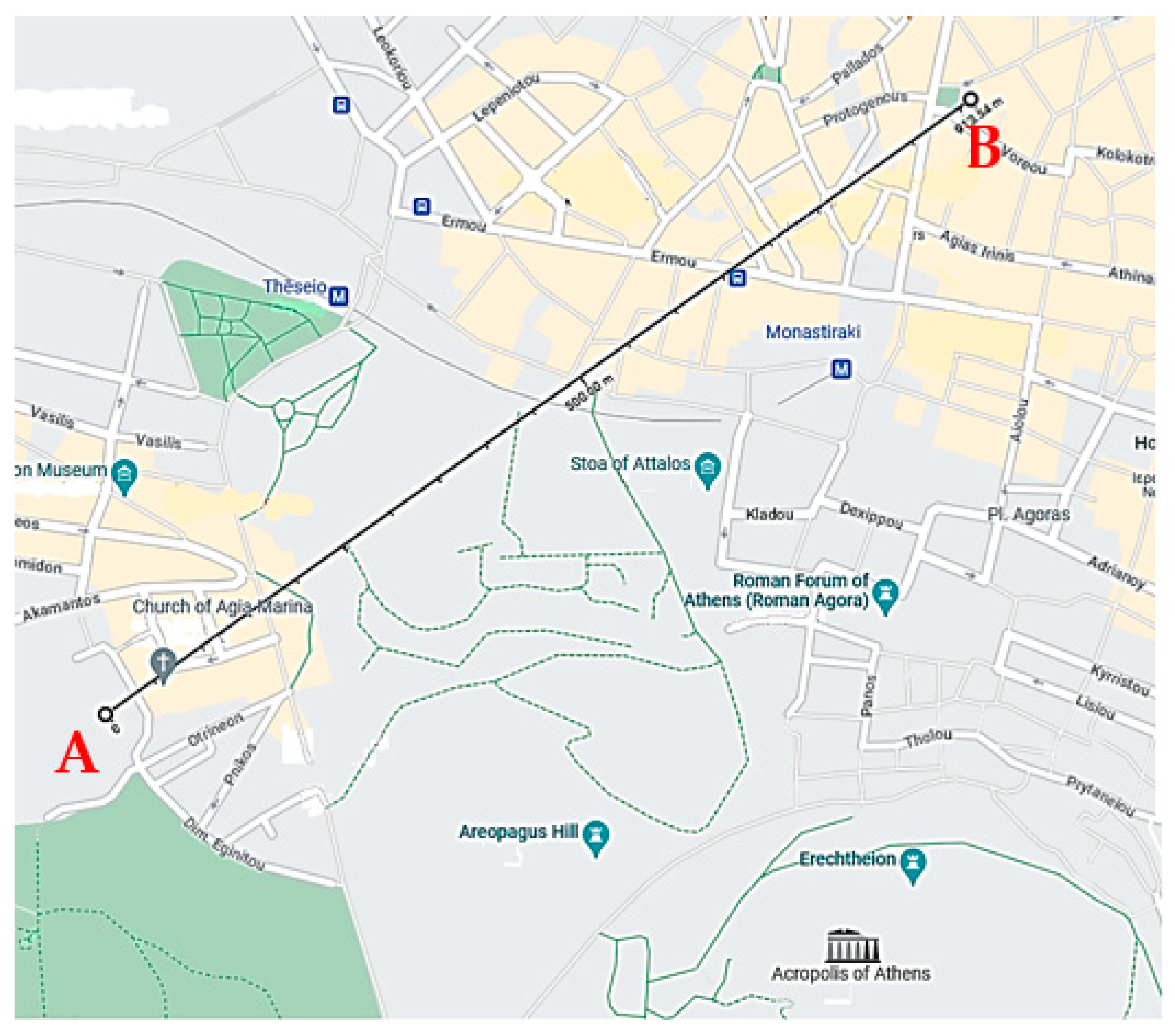
3.1. System Overview

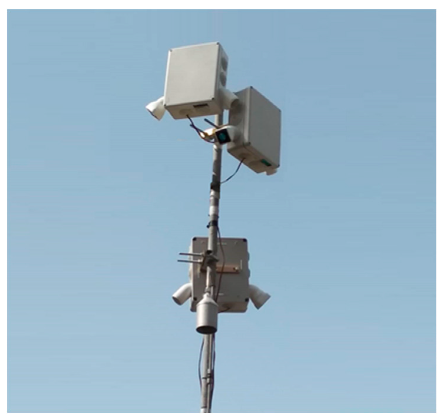
For first time in April 2021, the air quality monitoring system developed was installed at the center area of Athens, Greece at a location which is denoted as point A in Figure 2. The values of the measurements performed were compared to the corresponding data, which were obtained from the website of the Ministry of Environment and Energy of Greece (PERPA) [70]. These reference data were derived from the measurements performed by the official pollution measuring stations of PERPA, which are placed also in the center area of Athens at a location denoted as point B in Figure 2. The distance between these two locations is 900 m. Both locations share the same urban conditions. Actually, the spatial coverage of a monitoring site represents the quantification of the variability of concentrations of a specific pollutant around the site [71,72], while the assessment of representativeness aims at the delimitation of areas of the concentration field with similar characteristics at specific locations, as well the spatial surrogate data (similar emission sources and land-cover characteristics) [73,74,75].

A synoptic overview of the overall system developed is illustrated in Figure 3.

As illustrated in Figure 3, the data acquisition was carried out by three sensor nodes, which namely are: AC_NO2_O3_1, AC_NO2_O3_2, and AC_NO2_O3_3. Their names represent the location (i.e., Athens Center), the gases they detect (i.e., NO₂ and O₃) and the node’s identification number. Each one of them incorporated both a NO₂ sensor and an O₃ sensor couple in order to measure the concentrations of these two chemical substances in ambient air. Each sensor node also incorporates a General Packet Radio Service (GPRS) unit and a Wi-Fi unit. By alternately using these modules, each node could correspondingly send sensed data to the Internet either across cellular communication networks via a GPRS base station or across Wi-Fi via an access point. Next, the data transmitted via the Internet reached an application server that runs under the Linux operating system. In this server, data processing and data visualization to the end user took place via an application that had been appropriately developed by using the Grafana open-source interactive visualization platform. Finally, the storage of the sensed data was performed in a database that was developed by using the influxDB open-source time-series database platform.

3.2. Sensor Nodes

As aforementioned, the system developed used three sensor nodes. They are displayed in Figure 4.

Each one of the three sensor nodes consisted of a microcontroller with high processing power, low power consumption and a sufficient number of ports for peripherals, i.e., sensors, Wi-Fi and GPS. The interior of one of the three nodes is displayed in Figure 5, while more details on their design and implementation can be found in [76].

3.3. Sensor Calibration

At the beginning of the experimental process, a couple of brand-new electrochemical sensors were incorporated in each one of the sensor nodes. The specific sensors were namely: Alphasense OX-B431 [77] for O₃ and Alphasense NO2-B43F for NO₂ [78]. Both of these sensors generally consisted of four electrodes supported by an individual sensor board (ISB).

These sensors provided the output measurements in mV range, corresponding to the concentration of the measured gas and any potential cross-sensitivity. Cross-sensitivity is defined as the chemical reaction of the measuring element by another gas other than the target gas, with the result that the measurements of an electrochemical sensor are affected. The cross-sensitivity from other gases can be seen in the technical specifications of the manufacturer datasheet of the ozone sensor (OX-B431) [75] and of the nitrogen dioxide sensor (NO2-B43F) [76].

Specifically, the NO₂ sensor (NO2-B43F) presented cross-sensitivity (% measured gas @5 ppm) for the gases H₂S < −80, NO < 5, CI₂ < 100, SO₂ < −3, and CO < −3; (% measured gas @100 ppm) for the gases H₂ < 0.1, C₂H₄ < 0.1, NH₃ < 0.5, and halothane (not detected). Similarly, the O₃ sensor (OX-B431) presented cross-sensitivity (% measured gas @5 ppm) for the gases H₂S < −80, NO < 5, CI₂ < 100, SO₂ < −3, and CO < −3; (% measured gas @100 ppm) for the gases H₂ < 0.1, C₂H₄ < 0.1, NH₃ < 0.5, and halothane <0.1.

In order to be able to read the gas concentration in each low-cost sensor, the manufacturer provides a set of steps that must be followed in order to perform an initial calibration. These steps take into consideration two factors for each sensor—the interface board and the electrodes—as well as environmental conditions such as the temperature. After this initial calibration is completed, further data elaboration is required to correct the calibrated data using known environmental measurements, and thus improve the accuracy of the extracted results.

Regarding the initial calibration of its sensors, Alphasense proposes several potential functions in its Application Note AAN-803-01 [79]. In the system developed in this specific research work, Equation (1) was selected to perform the initial calibration of the sensors used. Specifically, Equation (1) provides the calibrated voltage output (i.e., WE_c: working electrode corrected) that finally represents the concentration of the gas detected, using the provided sensitivity of each individual sensor. This step incorporates the measured working electrode reading (WE_u), the auxiliary electrode reading (AE_u), and a temperature parameter n_T according to Application Note AAN 803-01. To complete the calibration for each individual sensor and ISB, Alphasense provides a set of background electrode noise values, corresponding to working electrode electronic zero (WE_e) and auxiliary electrode electronic zero (AE_e), which are also indicated in Equation (1):

WE_c = (WE_u − WE_e) − n_T × (AE_u − AE_e)

(1)

The gas pollutant concentration measurement of x gas is given by dividing the calibrated voltage output (i.e., WE_c: working electrode corrected) by the Sensor_{_Sensitivity}, as shown in Equation (2):

GASx_m = WE_c/Sensor_{_Sensitivity}

(2)

where GASx_m is the corrected measurement concentration, WE_c is the calibrated value of x gas (see Εquation (1)), and the sensor sensitivity is given by the manufacturer for each sensor.

Following the above procedure and according to the manufacturer, a methodology must be designed and followed by the end user in order to improve calibration by taking into consideration the impact of temperature, aging, etc. In this research work, after various attempts, the corrective formula that was found to fit best the corresponding values of the official instrumentation installed (i.e., the measuring stations of PERPA, Point B) [70] is the one described by Equation (3):

GASx_c = (GASx_m + C1)/C2

(3)

where GASx_c is the corrected value of x gas and GASx_m is the value of the measured concentration of x gas after applying Equation (2), while C1 and C2 are coefficients calculated for each station individually after a period of operation in the field, side by side with the reference equipment.

Using Equation (3), the values of GASx_c are expressed in ppb. The conversion from ppb to µg/m³ is achieved by multiplying the gas concentration in ppb by the conversion factors, for an ambient pressure of 1 atmosphere and a temperature of 20 degrees Celsius. The conversion factors are, for ozone (O₃) 1.995, and for nitrogen dioxide (NO₂) 1.912. It must be noted that regarding NO₂ the correction coefficient C2 obtains three distinct values depending on the level of NO₂ concentration. Following the procedure of correction, the three coefficients are calculated as C2a, when ${\mathrm{N}\mathrm{O}}_2<3$, C2b, when $3\le {\mathrm{N}\mathrm{O}}_2\le 30$ and C2c, when ${\mathrm{N}\mathrm{O}}_2>30$.

4. Experimental Procedure Results and Discussion

Based on the aforementioned calibration and correction procedure in Section 3, several experiments were conducted in order to verify the impact of aging on the corrective formula expressed by Equation (3).

Specifically, during the period of calibration and initial correction (i.e., 14 April 2021 to 10 May 2021) the temporal variation of the corrected NO₂ and O₃ values of the three nodes for the corresponding values of the reference instruments are illustrated in Figure 6 and Figure 7, respectively. Henceforth, the corrected values calculated for the three nodes are plotted in scatter correlation plots to evaluate the conversion performance.

Observing Figure 6 and Figure 7, it is obvious that the corrected values of the measurements from low-cost sensors tend to follow the corresponding values of the reference instruments. Observing Figure 7, it becomes evident that the low-cost sensors failed to reach the minimum values when these were obtained from the reference instruments. This can be attributed to the cross sensitivity of the sensor that was activated from other existing environmental oxides. In Figure 8a–c, the cross-correlation performance of the calibration and correction regarding the NO₂ measurements of the three nodes is depicted. The corresponding behavior for the O₃ measurements is shown in Figure 9a–c. Both Figure 8 and Figure 9 evince the consistency of the sensors. It is observed that C1 coefficient shows linear correlation. The expected temporal limitation of the C1 trend is significantly longer than the 2-year lifetime of the sensors, as provided by the manufacturers.

After the evaluation of the low-cost sensors and the validation of the high degree of cross-correlation, the measurements of the low-cost sensors were compared against the measurements of reference instruments as depicted in Figure 10a,b. For simplicity reasons henceforth the data of only one of the low-cost sensors are presented in the plots to provide the degree of cross-correlation. Figure 10a,b show the correlation for the NO₂ and O₃ concentration between the low-cost node AC_NO2_O3_2 and the reference instruments for the period of training (i.e., April 2021). In addition,

Table 1. Coefficients C1 and C2 for the low-cost NO₂ and O₃ gas sensors of the three nodes during all the period studied.

Gas	Node	April 2021				July 2021				October 2021				December 2021
		C1	C2			C1	C2			C1	C2			C1	C2
			a	b	c		a	b	c		a	b	c		a	b	c
NO2	AC_NO2_O3_1	50	15	2.2	1	47	15	3.5	1.2	43	15	3.5	1	41	15	2	1
	AC_NO2_O3_2	50	15	2	1	47	15	2.5	1	44	15	3.3	2	42	15	2.5	1
	AC_NO2_O3_3	74	15	2.4	1.5	72	15	3.4	1	69	15	3.5	1	67	15	3	1
		C1		C2		C1		C2		C1		C2		C1		C2
O3	AC_NO2_O3_1	43		1.8		45		2.8		48		2.4		50		2
	AC_NO2_O3_2	45		1.8		47		2.5		49		2.1		51		2
	AC_NO2_O3_3	40		1.7		43		2.4		45		3		47		1.6

summarizes the values of coefficients C1 and C2. Specifically for NO, the coefficient C2 is divided into three sub-coefficients C2a, C2b, C2c according to the measurement of the concentration of nitrogen dioxide) for all the low-cost measurement stations for all the tests that were conducted to evaluate the correlation, correction, and aging involution functions.

Next, the time dependent deviation from accuracy was studied using the protocol:

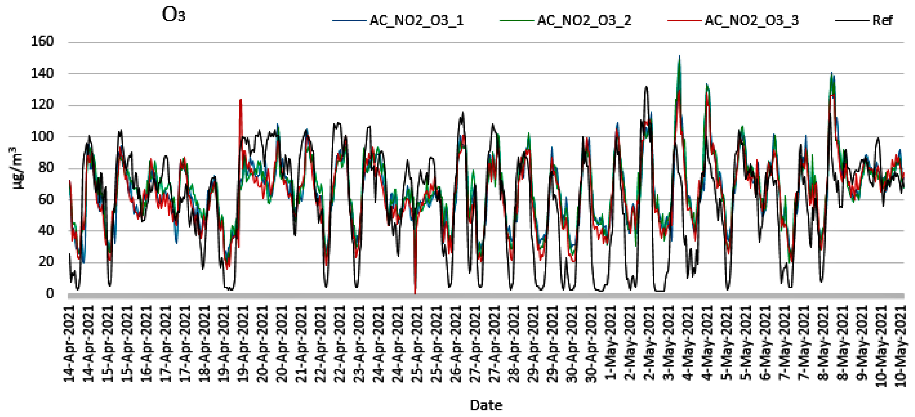
• The values of C1 and C2 were maintained as constant and the correlation degree R² was studied between the reference instruments and the low-cost stations during July 2021, October 2021 and December 2021. The results in this step are presented in

  Table 2. Correlation results between the reference instruments and the low-cost sensors while C1 and C2 are kept constant and equal to those calculated during the installation of nodes.

  Nodes	Coeff.	April 2021		July 2021		October 2021		December 2021
  		NO2	O3	NO2	O3	NO2	O3	NO2	O3
  AC_NO2_O3_1	A	0.8151	0.4625	−0.3521	0.826	0.7902	0.5071	0.4829	0.531
  	B	11.408	39.326	50.281	63.485	13.657	39.892	39.602	25.26
  	R2	0.4889	0.5506	0.0529	0.1963	0.3864	0.6494	0.4511	0.679
  AC_NO2_O3_2	A	0.9373	0.5156	−0.2162	0.7511	0.7648	0.4751	0.3962	0.466
  	B	4.2728	33.426	31.447	62.033	39.329	30.472	27.553	13.46
  	R2	0.6959	0.6141	0.0375	0.1717	0.1619	0.5399	0.3326	0.217
  AC_NO2_O3_3	A	0.8897	0.4658	−0.1519	0.788	0.3447	0.3995	0.3266	0.488
  	B	2.0495	38.05	32.619	57.386	9.5425	75.144	30.408	21.56
  	R2	0.7	0.5364	0.0161	0.2617	0.2388	0.4625	0.2448	0.706

  , manifesting the gradual deterioration of R².

Additionally, in Table 2 the reference/low-cost correlation fitting is presented as equation, y = αx + b, where y is the dependent variable (reference instrument μg/m³ value), α is the regression coefficient, x (low-cost station μg/m³ value) is the independent variable and b is a constant. Observing the above findings, it becomes evident that the performance of the sensing stations gradually deteriorates as the R² is decreased over time. For this reason, it was decided to make a temporal change on the C1 and C2 and re-examine the performance of the sensing device.

It becomes evident from Table 2 that NO₂ values during July show low cross-correlation. As will be discussed later on, the impact of the aging compensation equations on the NO₂ value is positive, as it improves the corresponding R² despite the fact that it remains at low values. Furthermore, in Greece, during the summertime, the environmental temperature pushes the sensors to their functional limits. Specifically, according to the manufacturer, these sensors are operational at the temperature range between −20 °C and 50 °C.

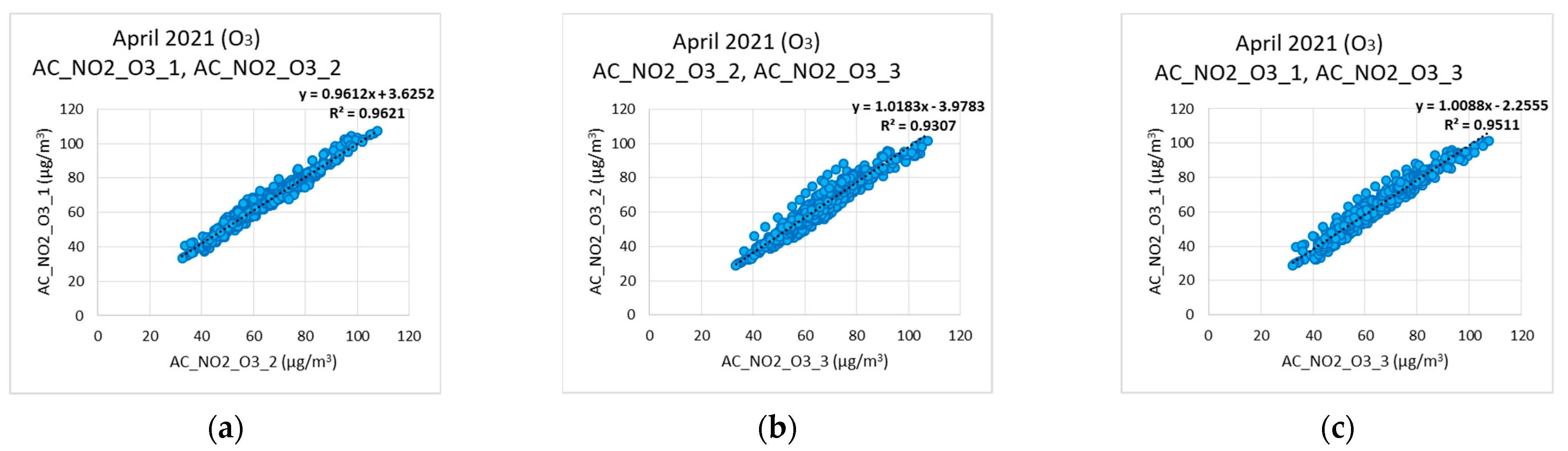
• New individual values for C1 and C2 were calculated (different ones for each period of study, i.e., July 2021, October 2021 and December 2021) and the new R² was calculated, indicating the temporal variation of C1 and C2 for both gases during their aging. The results extracted are displayed in

  Table 3. Summary of the correlation results among the reference instruments and the low-cost sensors while the coefficients C1 and C2 vary and are recalculated according to the aging functions (indicated by Equations (4) and (5)).

  Nodes	Coeff.	April 2021		July 2021		October 2021		December 2021
  		NO2	O3	NO2	O3	NO2	O3	NO2	O3
  AC_NO2_O3_1	A	0.8151	0.4625	−0.2377	0.5311	0.6429	0.3718	0.4322	0.477
  	B	11.408	39.326	37.704	42.24	8.7848	34.555	27.746	29.72
  	R2	0.4889	0.5506	0.0565	0.1961	0.4058	0.6325	0.4067	0.678
  AC_NO2_O3_2	A	0.9373	0.5156	−0.2236	0.5409	0.5061	0.4081	0.4293	0.481
  	B	4.2728	33.426	29.386	46.249	23.494	29.889	16.356	15.89
  	R2	0.6959	0.6141	0.057	0.1718	0.1551	0.5402	0.4733	0.468
  AC_NO2_O3_3	A	0.8897	0.4658	−0.1616	0.5583	0.3382	0.2284	0.5357	0.517
  	B	2.0495	38.05	32.57	43.127	10.227	45.797	12.01	31.65
  	R2	0.7	0.5364	0.0282	0.2617	0.2496	0.4642	0.4954	0.705

  . In addition, in Table 3 the reference/low-cost correlation fitting is presented as equation, y = αx + b, where y is the dependent variable (reference instrument μg/m³ value), α is the regression coefficient, x (low-cost station μg/m³ value) is the independent variable, and b is a constant.

The extracted results from Table 2 and Table 3 are shown at Figure 11 and Figure 12. Figure 11 shows the correlations (R²) of NO₂ and O₃ low-cost sensor measurements and reference, for the months July, October, and December 2021 with the calculated coefficients C1 and C2 of April, as well as the correlations of NO₂ and O₃ measurements, for the months July, October, and December 2021 with the calculated coefficients C1 and C2 of each month.

Figure 12 shows coefficients A and B of equation Y = AX + B for the NO₂ and O₃ measurements for July, October, and December 2021, by applying calculated coefficients C1 and C2 for April as well as calculated coefficients C1 and C2 of each month.

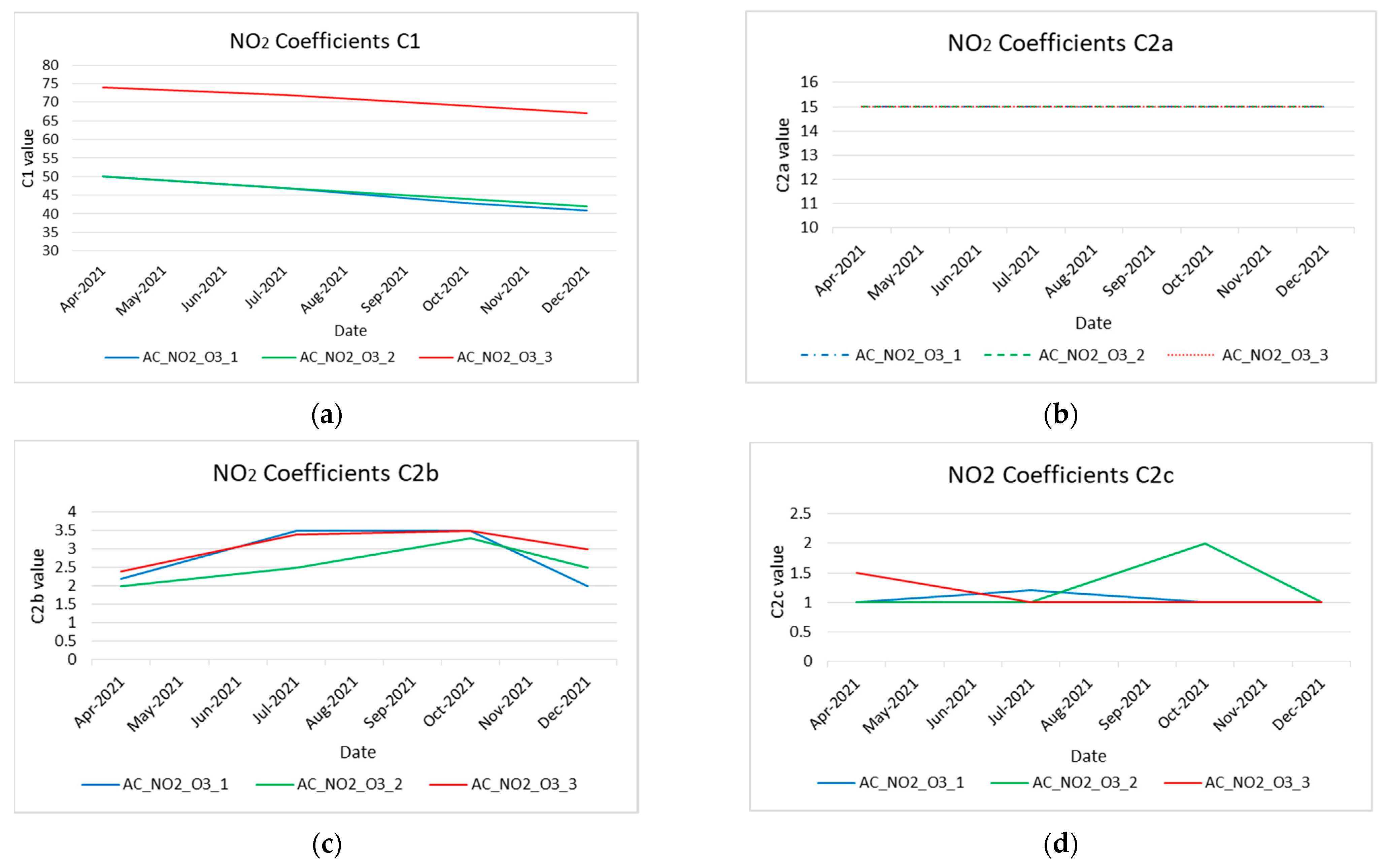
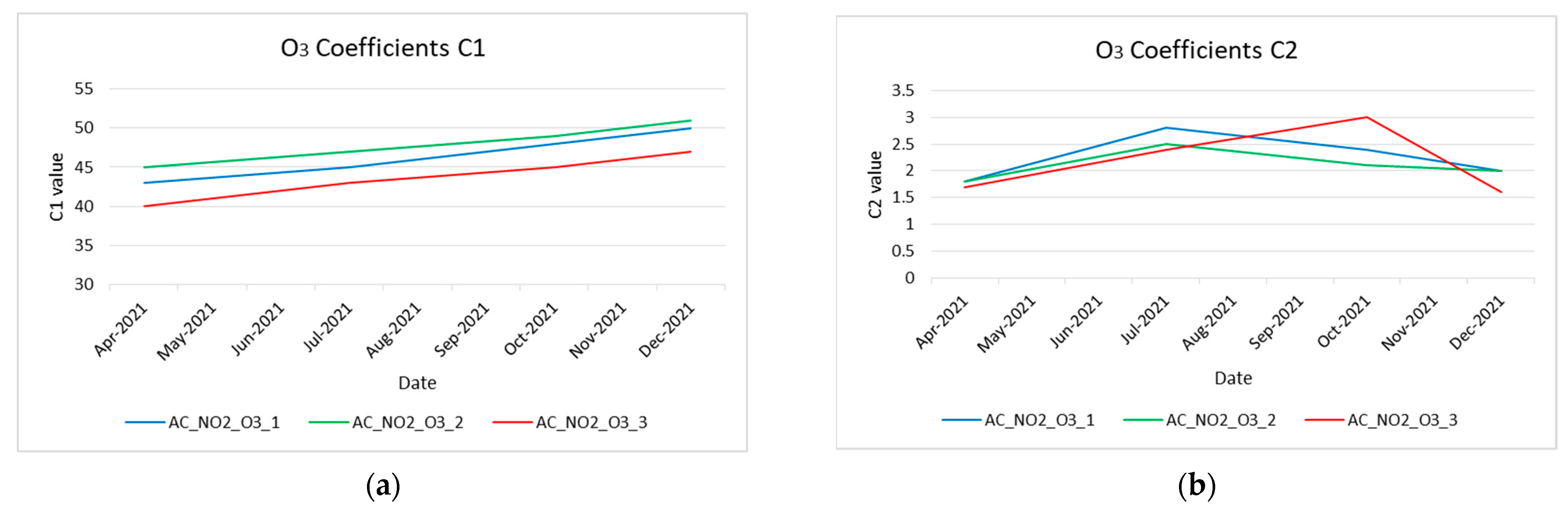
• Observation of the variation of C1 and C2 fitting was made to obtain the temporal variation of C1 and C2 and extrapolate all intermediate values. While performing this last step in order to obtain the aging formula, it was observed that coefficient C1 for NO₂ during the operation of the sensors showed a decrease by one unit per month of the initial value from the beginning of the operation of the sensor. Next, coefficient C1 concerning the aging of the sensor was introduced as ${\mathrm{C}1}_{\mathrm{A}\mathrm{g}\mathrm{e}}$. In this way, the coefficient ${\mathrm{C}1}_{\mathrm{A}\mathrm{g}\mathrm{e}}$ for NO₂ sensor is described in Equation (4) and the corresponding behavior for the O₃ sensor is described in Equation (5)

$${\mathrm{C}1}_{\mathrm{A}\mathrm{g}\mathrm{e}}\left({\mathrm{NO}}_2\right)={\mathrm{C}1}_{\mathrm{i}\mathrm{n}\mathrm{i}\mathrm{t}}\left({\mathrm{NO}}_2\right)-\mathrm{n}$$

(4)

$${\mathrm{C}1}_{\mathrm{A}\mathrm{g}\mathrm{e}}\left({\mathrm{O}}_3\right)={\mathrm{C}1}_{\mathrm{i}\mathrm{n}\mathrm{i}\mathrm{t}}\left({\mathrm{O}}_3\right)+\mathrm{n}$$

(5)

where ${\mathrm{C}1}_{\mathrm{i}\mathrm{n}\mathrm{i}\mathrm{t}}$ represents the initial value of the coefficient from the beginning of the sensor’s operation, and n expresses the sum of the months of in-time service of the sensor.

Next, the temporal variation of all coefficients (i.e., C1, C2x) was plotted to evaluate the aging functions’ performance. The extracted results are depicted in Figure 13a–d for NO₂ sensors and Figure 14a,b for O₃ sensors. These figures prove the variability of C1 and C2 during the operation time (8 months) of the sensors.

Both in the nitrogen dioxide sensors and in the ozone sensors, it is observed that the C1 coefficient shows a linearity, which is expected according to the manufacturer; the sensor during its lifetime (about two years) operates in a linear range.

Coefficient C2 concerns the scale of the measured values in relation to aging of the sensor. According to the datasheets of O₃ [77] and NO₂ [78] sensors, their sensitivity depends on the temperature [79]. The mean temperature values per month in 2021 in the center of Athens are presented in

Table 4. Annual climatological summary for 2021 [80].

Annual Climatological Summary
Name: athens984 City: Athens State: Attica, Greece
Elev: 60m Lat: 37°58′42″ N Long: 23°42′56″ E
Temperature (°C), Hheat Base 18.3, Cool Base 18.3
Year	Month	Mean MAX	Mean MIN	Mean
2021	1	15.0	7.9	11.5
2021	2	15.8	7.0	11.3
2021	3	16.2	8.3	12.1
2021	4	20.0	11.3	15.7
2021	5	27.3	17.8	22.4
2021	6	30.1	21.1	25.4
2021	7	34.1	25.9	29.9
2021	8	34.3	25.5	29.7
2021	9	28.5	20.5	24.2
2021	10	21.7	15.0	18.0
2021	11	19.1	12.6	15.7
2021	12	14.9	8.3	11.7

, where the average temperatures for the months that the experiment took place are highlighted [80].

Coefficient C2 (referred as ${\mathrm{C}2}_{\mathrm{S}\mathrm{c}\mathrm{a}\mathrm{l}\mathrm{e}}$) contrary to ${\mathrm{C}1}_{\mathrm{A}\mathrm{g}\mathrm{e}}$ is not so closely related to the sensor lifetime. Instead, ambient temperature severely impacts the recordings of sensors. This is not only observed but is also stated by the sensor manufacturer. Thus, ${\mathrm{C}2}_{\mathrm{S}\mathrm{c}\mathrm{a}\mathrm{l}\mathrm{e}}$ is the corrected value after taking into consideration the temperature according to [75,77]. Coefficient ${\mathrm{C}2}_{{\mathrm{S}\mathrm{c}\mathrm{a}\mathrm{l}\mathrm{e}(\mathrm{O}}_3)}$ for O₃ measurements is given by Equation (6):

$${\mathrm{C}2}_{{\mathrm{S}\mathrm{c}\mathrm{a}\mathrm{l}\mathrm{e}(\mathrm{O}}_3)}={\mathrm{C}2}_{{\mathrm{i}\mathrm{n}\mathrm{i}\mathrm{t}(\mathrm{O}}_3)}+({\mathrm{S}}_{\mathrm{i}\mathrm{n}\mathrm{i}\mathrm{t}}-{\mathrm{S}}_{\mathrm{c}\mathrm{u}\mathrm{r}\mathrm{r}\mathrm{e}\mathrm{n}\mathrm{t}})/10$$

(6)

where ${\mathrm{C}2}_{{\mathrm{i}\mathrm{n}\mathrm{i}\mathrm{t}(\mathrm{O}}_3)}$ is the initial value of C2 from the beginning of the O₃ sensor operation, ${\mathrm{S}}_{\mathrm{init}}$ is the sensitivity of the sensor during the first day of its lifetime at a specific temperature and ${\mathrm{S}}_{\mathrm{current}}$ is the corresponding sensitivity at the temperature of the running month [77]. As described in Table 1 the coefficients ${\mathrm{C}2\mathrm{a}}_{{\mathrm{S}\mathrm{c}\mathrm{a}\mathrm{l}\mathrm{e}(\mathrm{N}\mathrm{O}}_2)}$ (NO₂ < 3) and ${\mathrm{C}2\mathrm{c}}_{{\mathrm{S}\mathrm{c}\mathrm{a}\mathrm{l}\mathrm{e}(\mathrm{N}\mathrm{O}}_2)}$ (3 < NO₂ < 30) are maintained practically constant where ${\mathrm{C}2\mathrm{a}}_{{\mathrm{S}\mathrm{c}\mathrm{a}\mathrm{l}\mathrm{e}(\mathrm{N}\mathrm{O}}_2)}$ = 15 and ${\mathrm{C}2\mathrm{c}}_{{\mathrm{S}\mathrm{c}\mathrm{a}\mathrm{l}\mathrm{e}(\mathrm{N}\mathrm{O}}_2)}$ = 1. Contrary to the above, the coefficient ${\mathrm{C}2\mathrm{b}}_{{\mathrm{S}\mathrm{c}\mathrm{a}\mathrm{l}\mathrm{e}(\mathrm{N}\mathrm{O}}_2)}$ (NO₂ > 30) is strongly affected by the temperature. The coefficient ${\mathrm{C}2\mathrm{a}}_{{\mathrm{S}\mathrm{c}\mathrm{a}\mathrm{l}\mathrm{e}(\mathrm{N}\mathrm{O}}_2)}$ for ΝO₂ measurements is given by Equation (7):

$${\mathrm{C}2}_{{\mathrm{S}\mathrm{c}\mathrm{a}\mathrm{l}\mathrm{e}(\mathrm{N}\mathrm{O}}_2)}={\mathrm{C}2}_{\mathrm{init}{(\mathrm{N}\mathrm{O}}_2)}+({\mathrm{S}}_{\mathrm{i}\mathrm{n}\mathrm{i}\mathrm{t}}-{\mathrm{S}}_{\mathrm{c}\mathrm{u}\mathrm{r}\mathrm{r}\mathrm{e}\mathrm{n}\mathrm{t}})/10$$

(7)

where ${\mathrm{C}2}_{{\mathrm{i}\mathrm{n}\mathrm{i}\mathrm{t}(\mathrm{N}\mathrm{O}}_2)}$ is the initial value of the coefficient from the beginning of the ΝO₂ sensor operation, ${\mathrm{S}}_{\mathrm{i}\mathrm{n}\mathrm{i}\mathrm{t}}$ is the sensitivity of the sensor during the first day of its lifetime at a specific temperature, and ${\mathrm{S}}_{\mathrm{c}\mathrm{u}\mathrm{r}\mathrm{r}\mathrm{e}\mathrm{n}\mathrm{t}}$ is the corresponding sensitivity at the temperature of the running month [78]. For each sensor, the corresponding datasheets provided by the manufacturer [75,76] include a graph which describes the relation of sensor sensitivity according to the temperature of the environment. The calculation of the corresponding sensitivity at a specific temperature is achieved by extracting the slope of the graph at each temperature case.

After having performed the above process, it was concluded that Equations (4)–(7) had an obvious impact on the performance of the sensors. Specifically, it was observed that the performance of the sensors was kept practically stable during their lifetime with respect to the corresponding results extracted when the C1 and C2 factors were maintained as initially set during their calibration. It could be seen that the adoption of a continuous correction process was required in order to maintain the validity of pollutant gas measurements.

To proceed in further evaluation of the initial calibration and the correction process due to aging, a boxplot presentation method was adopted. Actually, a boxplot, also known as a box and whisker plot, is a graphical representation of statistical data that displays the distribution of a dataset by showing the median, quartiles, and range of the data. Boxplots are useful for both comparing the distribution of different datasets and visualizing the distribution of a single dataset. They can also help to identify any potential outliers in the data.

Specifically, the boxplots depicted in Figure 15 show the variation of the measured quantities, between the inexpensive and reference sensors. Figure 15a illustrates the O₃ variation for October 2021 using the coefficients C1 and C2 that were calculated for April 2021, while Figure 15b shows the corresponding variation using the coefficients calculated using the data from October 2021. Figure 15c and Figure 15d, respectively, show the correction degree using the coefficients C1 and C2 for NO₂.

Observing the results in the boxplots illustrated in Figure 15, it can be straight forwardly concluded that the deviation of the recorded values with respect to the reference instruments were significantly lower when changing the C1 and C2 coefficients (see Figure 15b,d) when compared to the corresponding deviation when using the same C1 and C2 values during the sensors’ lifetime (see Figure 15a,c). This fact supports the need for adopting changes for the correction process during the lifetime of a low-cost electrochemical sensor. Furthermore, it becomes obvious that the adopted Equations (4)–(7) can improve the performance of the sensors during their lifetime instead of keeping their values constant during the lifetime of the sensors. It is still remaining to study whether these equations can be further improved.

Finally, in order to demonstrate the impact of the change on the coefficients on the performance, the corresponding boxplots were plotted and are shown in Figure 16. Figure 16a–h show the variation of NO₂ and O₃ for each month for the coefficients C1 and C2 recalculated according to the aging formulas for each one of the studied months. Specifically, Figure 16a,b correspond to the statistical variation of the reference/low-cost using the aging-corrected C1 and C2 for NO₂ and O₃ during April 2021 (period A). The corresponding box plots for July 2021 (period B) are depicted in Figure 16c,d. The October 2021 (period C) corresponding results are presented in Figure 16e,f for NO₂ and O₃, respectively. Lastly, the extracted statistical boxplot results regarding December of 2021 (period D) are shown in Figure 16g,h.

Observing Figure 16, it becomes obvious that the use of the methodology proposed in this article is indeed not only essential but also very effective in keeping the performance of inexpensive electrochemical sensors constant during their lifetime.

5. Conclusions

There is no doubt that air quality monitoring in urban environments is one of the most important applications of WSNs in smart cities. It is also true that there are many commercially available instruments that are able to perform air quality monitoring with high accuracy. However, they are very expensive to use in large-scale installations. At the same time, technological advances have made it feasible to mass-manufacture inexpensive electrochemical sensors that are able to measure the concentrations of pollutant gases in air with relatively good accuracy. On the other hand, aging caused by a variety of factors, including exposure to high levels of gases, temperature fluctuations, and moisture, deteriorates the sensitivity of such sensors, leading to inaccurate readings. One common way to address sensor aging is to periodically perform calibration of the sensors in order to check the existing accuracy and properly improve it if needed. Actually, most of the published works that deal with the aging of low-cost sensors involve machine learning, neural networks, and other similar processing-demanding methods. Such approaches require significant CPU and memory resources, having a direct impact on the processing capability specifications and the cost of such a measuring system. Additionally, incorporating such methodologies on the measuring unit significantly increases energy consumption. Even for the case when the processing is conducted at a central point, the need for high processing power remains, since each networked measuring system must be treated separately. The herein proposed solution incorporates a simple compensation algorithm of good performance that can be easily executed at any sensing node. In addition, due to the simplicity of the required actions, power consumption is practically unaffected.

Specifically, in this research work, the impact of aging on the accuracy of low-cost gaseous pollutant sensors used in WSNs was studied. Specifically, an air quality monitoring WSN containing three sensor nodes was established in the center of Athens, Greece. Each one of the specific sensor nodes encompassed a couple of sensors that monitored the concentration of ozone and nitrogen dioxide in the ambient air. For a period of eight months the values of the measurements of these sensors were compared with those made by the air monitoring instruments that are officially used by the State.

The first conclusion drawn from this research work is that the sensor’s aging—which may be caused by a variety of factors, including exposure to high levels of gases, temperature fluctuations, and moisture—indeed impacts its sensitivity, leading to inaccurate readings. One common way to address sensor aging is to periodically calibrate the sensors to ensure their accuracy.

However, this research work evinced that there is a very effective methodology to keep the sensors’ performance stable during their lifecycle. Actually, coefficients C1 and C2 used in the methodology proposed express the performance of a sensor during its operational life. Specifically, coefficient C1 is directly related to aging and its value changes for each month of the operational time of the sensor according to a formula which is differentiated according to the pollutant gas detected. At the same time, coefficient C2 aims at the micrometric correction of the sensor values according to the average temperature of the month of operation under study.

The suitable use of these two coefficients in the formulae proposed showed excellent results for both NO₂ and O₃ low-cost air quality sensors, in the sense that not only their aging was treatable but also high reliability of the measurements can be achieved for the entire lifetime of the sensors. In this way, air quality monitoring can be performed via low-cost sensors with no need for recalibration with official reference instruments at regular intervals. So, it is feasible to create dense air quality monitoring networks in urban areas without high acquisition costs. This is greatly beneficial to the attainment of not only inexpensive but also accurate air monitoring via WSNs in smart cities.

References

1. Judy, J.W. Microelectromechanical Systems (MEMS): Fabrication, Design and Applications. Smart Mater. Struct. 2001, 10, 1115–1134. [Google Scholar] [CrossRef] [Green Version]
2. Akyildiz, I.F.; Su, W.; Sankarasubramaniam, Y.; Cayirci, E. A Survey on Sensor Networks. IEEE Commun. Mag. 2002, 40, 104–112. [Google Scholar] [CrossRef] [Green Version]
3. Yick, J.; Mukherjee, B.; Ghosal, D. Wireless Sensor Network Survey. Comput. Netw. 2008, 52, 2292–2330. [Google Scholar] [CrossRef]
4. Evangelakos, E.A.; Kandris, D.; Rountos, D.; Tselikis, G.; Anastasiadis, E. Energy Sustainability in Wireless Sensor Networks: An Analytical Survey. J. Low Power Electron. Appl. 2022, 12, 65. [Google Scholar] [CrossRef]
5. Nakas, C.; Kandris, D.; Visvardis, G. Energy Efficient Routing in Wireless Sensor Networks: A Comprehensive Survey. Algorithms 2020, 13, 72. [Google Scholar] [CrossRef] [Green Version]
6. Farsi, M.; Elhosseini, M.A.; Badawy, M.; Arafat Ali, H.; Zain Eldin, H. Deployment Techniques in Wireless Sensor Networks, Coverage and Connectivity: A Survey. IEEE Access 2019, 7, 28940–28954. [Google Scholar] [CrossRef]
7. Kandris, D.; Vergados, D.J.; Vergados, D.D.; Tzes, A. A Routing Scheme for Congestion Avoidance in Wireless Sensor Networks. In Proceedings of the 6th Annual IEEE Conference on Automation Science and Engineering (CASE 2010), Toronto, ON, Canada, 21–24 August 2010; pp. 21–24. [Google Scholar]
8. Ploumis, S.E.; Sgora, A.; Kandris, D.; Vergados, D.D. Congestion Avoidance in Wireless Sensor Networks: A Survey. In Proceedings of the 2012 16th Panhellenic Conference on Informatics, PCI 2012, Piraeus, Greece, 5–7 October 2012; pp. 234–239. [Google Scholar] [CrossRef]
9. Kandris, D.; Alexandridis, A.; Dagiuklas, T.; Panaousis, E.; Vergados, D.D. Multiobjective Optimization Algorithms for Wireless Sensor Networks. Wirel. Commun. Mob. Comput. 2020, 2020, 1–5. [Google Scholar] [CrossRef]
10. Sharma, N.; Singh, B.M.; Singh, K. QoS-Based Energy-Efficient Protocols for Wireless Sensor Network. Sustain. Comput. Inform. Syst. 2021, 30, 100425. [Google Scholar] [CrossRef]
11. Tarnaris, K.; Preka, I.; Kandris, D.; Alexandridis, A. Coverage and K-Coverage Optimization in Wireless Sensor Networks Using Computational Intelligence Methods: A Comparsative Study. Electronics 2020, 9, 675. [Google Scholar] [CrossRef] [Green Version]
12. Yu, J.Y.; Lee, E.; Oh, S.R.; Seo, Y.D.; Kim, Y.G. A Survey on Security Requirements for WSNs: Focusing on the Characteristics Related to Security. IEEE Access 2020, 8, 45304–45324. [Google Scholar] [CrossRef]
13. Kandris, D.; Nakas, C.; Vomvas, D.; Koulouras, G. Applications of Wireless Sensor Networks: An Up-to-Date Survey. Appl. Syst. Innov. 2020, 3, 14. [Google Scholar] [CrossRef] [Green Version]
14. Pantazis, N.A.; Nikolidakis, S.A.; Kandris, D.; Vergados, D.D. An Automated System for Integrated Service Management in Emergency Situations. In Proceedings of the 2011 Panhellenic Conference on Informatics, PCI 2011, Kastoria, Greece, 30 September–2 October 2011; pp. 154–157. [Google Scholar] [CrossRef]
15. Papadakis, N.; Koukoulas, N.; Christakis, I.; Stavrakas, I.; Kandris, D. An Iot-Based Participatory Antitheft System for Public Safety Enhancement in Smart Cities. Smart Cities 2021, 4, 919–937. [Google Scholar] [CrossRef]
16. Khedo, K.K.; Bissessur, Y.; Goolaub, D.S. An Inland Wireless Sensor Network System for Monitoring Seismic Activity. Future Gener. Comput. Syst. 2020, 105, 520–532. [Google Scholar] [CrossRef]
17. Nikolidakis, S.A.; Kandris, D.; Vergados, D.D.; Douligeris, C. Energy Efficient Automated Control of Irrigation in Agriculture by Using Wireless Sensor Networks. Comput. Electron. Agric. 2015, 113, 154–163. [Google Scholar] [CrossRef]
18. Farooq, M.U.; Waseem, M.; Mazhar, S.; Khairi, A.; Kamal, T. A Review on Internet of Things (IoT). Int. J. Comput. Appl. 2015, 113, 135–144. [Google Scholar] [CrossRef]
19. Ali, A. A Framework for Air Pollution Monitoring in Smart Cities by Using IoT and Smart Sensors. Informatica 2022, 46. [Google Scholar] [CrossRef]
20. Thangammal, C.B.; Ilamathi, K.; Poonkuzhali, P.; Aarthi, R. An IoT Enabled Air Quality Monitoring Mobile App for Smart Cities. In Proceedings of the 2nd International Conference on Recent Trends in Machine Learning, IoT, Smart Cities and Applications, Hyderabad, Telangana, India, 28–29 March 2021; pp. 275–285. [Google Scholar] [CrossRef]
21. Snyder, E.G.; Watkins, T.H.; Solomon, P.A.; Thoma, E.D.; Williams, R.W.; Hagler, G.S.W.; Shelow, D.; Hindin, D.A.; Kilaru, V.J.; Preuss, P.W. The Changing Paradigm of Air Pollution Monitoring. Environ. Sci. Technol. 2013, 47, 11369–11377. [Google Scholar] [CrossRef]
22. Kumar, P.; Morawska, L.; Martani, C.; Biskos, G.; Neophytou, M.; Di Sabatino, S.; Bell, M.; Norford, L.; Britter, R. The Rise of Low-Cost Sensing for Managing Air Pollution in Cities. Environ. Int. 2015, 75, 199–205. [Google Scholar] [CrossRef] [Green Version]
23. Balogun, A.-L.; Tella, A.; Baloo, L.; Adebisi, N. A Review of the Inter-Correlation of Climate Change, Air Pollution and Urban Sustainability Using Novel Machine Learning Algorithms and Spatial Information Science. Urban Clim. 2021, 40, 100989. [Google Scholar] [CrossRef]
24. Zhao, B.; Yu, L.; Wang, C.; Shuai, C.; Zhu, J.; Qu, S.; Taiebat, M.; Xu, M. Urban Air Pollution Mapping Using Fleet Vehicles as Mobile Monitors and Machine Learning. Environ. Sci. Technol. 2021, 55, 5579–5588. [Google Scholar] [CrossRef]
25. Lautenschlager, F.; Becker, M.; Kobs, K.; Steininger, M.; Davidson, P.; Krause, A.; Hotho, A. OpenLUR: Off-The-Shelf Air Pollution Modeling with Open Features and Machine Learning. Atmos. Environ. 2020, 233, 117535. [Google Scholar] [CrossRef]
26. Wang, A.; Xu, J.; Tu, R.; Saleh, M.; Hatzopoulou, M. Potential of Machine Learning for Prediction of Traffic Related Air Pollution. Transp. Res. Part D Transp. Environ. 2020, 88, 102599. [Google Scholar] [CrossRef]
27. Aditya, C.R.; Deshmukh, C.R.; Nayana, D.K.; Vidyavastu, P.G. Detection and prediction of air pollution using machine learning models. Int. J. Eng. Trends Technol. 2018, 59, 204–207. [Google Scholar]
28. Xi, X.; Zhao, W.; Rui, X.; Wang, Y.; Bai, X.; Yin, W.; Don, J. A comprehensive evaluation of air pollution prediction improvement by a machine learning method. In Proceedings of the 2015 IEEE International Conference on Service Operations and Logistics, and Informatics (SOLI), Yasmine Hammamet, Tunisia, 15–17 November 2015; pp. 176–181. [Google Scholar]
29. McKercher, G.R.; Salmond, J.A.; Vanos, J.K. Characteristics and Applications of Small, Portable Gaseous Air Pollution Monitors. Environ. Pollut. 2017, 223, 102–110. [Google Scholar] [CrossRef] [PubMed] [Green Version]
30. Lewis, A.; Peltier, W.R.; von Schneidemesser, E. Low-Cost Sensors for the Measurement of Atmospheric Composition: Overview of Topic and Future Applications; Research report; World Meteorological Organization: Geneva, Switzerland, 2018. [Google Scholar]
31. Cross, E.S.; Williams, L.R.; Lewis, D.K.; Magoon, G.R.; Onasch, T.B.; Kaminsky, M.L.; Worsnop, D.R.; Jayne, J.T. Use of Electrochemical Sensors for Measurement of Air Pollution: Correcting Interference Response and Validating Measurements. Atmos. Meas. Tech. 2017, 10, 3575–3588. [Google Scholar] [CrossRef] [Green Version]
32. Jerrett, M.; Donaire-Gonzalez, D.; Popoola, O.; Jones, R.; Cohen, R.C.; Almanza, E.; de Nazelle, A.; Mead, I.; Carrasco-Turigas, G.; Cole-Hunter, T.; et al. Validating Novel Air Pollution Sensors to Improve Exposure Estimates for Epidemiological Analyses and Citizen Science. Environ. Res. 2017, 158, 286–294. [Google Scholar] [CrossRef] [PubMed]
33. deSouza, P. A Nairobi Experiment in Using Low-cost Air Quality Monitors. Clean Air J. 2017, 27, 12–42. [Google Scholar] [CrossRef]
34. D’Alvia, L.; Palermo, E.; Del Prete, Z. Validation and application of a novel solution for environmental monitoring: A three month study at “Minerva Medica” archaeological site in Rome. Measurement 2018, 129, 31–36. [Google Scholar] [CrossRef]
35. Lewis, A.C.; Lee, J.D.; Edwards, P.M.; Shaw, M.D.; Evans, M.J.; Moller, S.J.; Smith, K.R.; Buckley, J.W.; Ellis, M.; Gillot, S.R.; et al. Evaluating the Performance of Low-cost Chemical Sensors for Air Pollution Research. Faraday Discuss. 2016, 189, 85–103. [Google Scholar] [CrossRef]
36. Christakis, I.; Syropoulou, P.; Papadakis, N.; Stavrakas, I. On the correction of low-cost NO2, O3 and PM sensors. In Proceedings of the Eighth International Conference on Environmental Management, Engineering, Planning & Economics, Thessaloniki, Greece, 20–24 July 2021; pp. 301–310. [Google Scholar]
37. Christakis, I.; Moutzouris, K.; Tsakiridis, O.; Stavrakas, I. Barometric Pressure as a correction factor for low-cost particulate matter sensors. In IOP Conference Series: Earth and Environmental Science; IOP Publishing: Athens, Greece, 2022; Volume 1123, No. 1. [Google Scholar]
38. Christakis, I.; Hloupis, G.; Tsakiridis, O.; Stavrakas, I. Integrated open source air quality monitoring platform. In Proceedings of the 11th International Conference on Modern Circuits and Systems Technologies (MOCAST), Bremen, Germany, 8–10 June 2022. [Google Scholar]
39. Williams, R.; Kilaru, V.; Snyder, E.; Kaufman, A.; Dye, T.; Rutter, A.; Russell, A. EPA Citizen Scientist Air Monitoring Tool Kit Air Sensor Guidebook; U.S. Environmental Protection Agency: Washington, DC, USA, 2014. [Google Scholar]
40. Gerboles, M.; Spinelle, L.; Borowiak, A. Measuring Air Pollution with Low-Cost Sensors. Thoughts on the Quality of Data Measured by Sensors; European Commission: Ispra, Italy, 2017. [Google Scholar]
41. Borrego, C.; Costa, A.M.; Ginja, J.; Amorim, M.; Coutinho, M.; Karatzas, K.; Sioumis, T.; Katsifarakis, N.; Konstantinidis, K.; De Vito, S.; et al. Assessment of Air Quality Microsensors versus Reference Methods: The EuNetAir Joint Exercise. Atmos. Environ. 2016, 147, 246–263. [Google Scholar] [CrossRef] [Green Version]
42. Mueller, M.; Meyer, J.; Hueglin, C. Design of an Ozone and Nitrogen Dioxide Sensor Unit and Its Long-Term Operation within a Sensor Network in the City of Zurich. Atmos. Meas. Tech. 2017, 10, 3783–3799. [Google Scholar] [CrossRef] [Green Version]
43. Samad, A.; Obando Nuñez, D.R.; Solis Castillo, G.C.; Laquai, B.; Vogt, U. Effect of Relative Humidity and Air Temperature on the Results Obtained from Low-Cost Gas Sensors for Ambient Air Quality Measurements. Sensors 2020, 20, 5175. [Google Scholar] [CrossRef] [PubMed]
44. Karagulian, F.; Barbiere, M.; Kotsev, A.; Spinelle, L.; Gerboles, M.; Lagler, F.; Redon, N.; Crunaire, S.; Borowiak, A. Review of the Performance of Low-Cost Sensors for Air Quality Monitoring. Atmosphere 2019, 10, 506. [Google Scholar] [CrossRef] [Green Version]
45. Pang, X.; Shaw, M.D.; Gillot, S.; Lewis, A.C. The Impacts of Water Vapour and Co-Pollutants on the Performance of Electrochemical Gas Sensors Used for Air Quality Monitoring. Sens. Actuators B Chem. 2018, 266, 674–684. [Google Scholar] [CrossRef]
46. Solis, G. Test and Analysis of Key Factors that Can Affect the Reliability of Results Obtained from Low-cost Sensors for Outdoor Air Quality Measurements. Master’s Thesis, University of Stuttgart, Stuttgart, Germany, 2019. [Google Scholar]
47. Bigi, A.; Mueller, M.; Grange, S.K.; Ghermandi, G.; Hueglin, C. Performance of NO, NO2 low-cost sensors and three calibration approaches within a real world application. Atmos. Meas. Tech. 2018, 11, 3717–3735. [Google Scholar] [CrossRef] [Green Version]
48. Williams, D.E. Electrochemical sensors for environmental gas analysis. Curr. Opin. Electrochem. 2020, 22, 145–153. [Google Scholar] [CrossRef]
49. Farquhar, A.K.; Henshaw, G.S.; Williams, D.E. Understanding and correcting unwanted influences on the signal from electrochemical gas sensors. ACS Sens. 2021, 6, 1295–1304. [Google Scholar] [CrossRef]
50. Wei, P.; Ning, Z.; Ye, S.; Sun, L.; Yang, F.; Wong, K.C.; Westerdahl, D.; Louie, P.K. Impact Analysis of Temperature and Humidity Conditions on Electrochemical Sensor Response in Ambient Air Quality Monitoring. Sensors 2018, 18, 59. [Google Scholar] [CrossRef] [PubMed] [Green Version]
51. Castell, N.; Dauge, F.R.; Schneider, P.; Vogt, M.; Lerner, U.; Fishbain, B.; Broday, D.; Bartonova, A. Can commercial low-cost sensor platforms contribute to air quality monitoring and exposure estimates? Environ. Int. 2017, 99, 293–302. [Google Scholar] [CrossRef]
52. Mead, M.I.; Popoola, O.A.M.; Stewart, G.B.; Landshoff, P.; Calleja, M.; Hayes, M.; Baldovi, J.J.; McLeod, M.W.; Hodgson, T.F.; Dicks, J.; et al. The use of electrochemical sensors for monitoring urban air quality in low-cost, high-density networks. Atmos. Environ. 2013, 70, 186–203. [Google Scholar] [CrossRef] [Green Version]
53. Pang, X.; Shaw, M.D.; Lewis, A.C.; Carpenter, L.J.; Batchellier, T. Electrochemical ozone sensors: A miniaturised alternative for ozone measurements in laboratory experiments and air-quality monitoring. Sens. Actuators B Chem. 2017, 240, 829–837. [Google Scholar] [CrossRef] [Green Version]
54. Sun, L.; Westerdahl, D.; Ning, Z. Development and Evaluation of a Novel and Cost-Effective Approach for Low-cost NO2 Sensor Drift Correction. Sensors 2017, 17, 1916. [Google Scholar] [CrossRef]
55. Piedrahita, R.; Xiang, Y.; Masson, N.; Ortega, J.; Collier, A.; Jiang, Y.; Li, K.; Dick, R.P.; Lv, Q.; Hannigan, M.; et al. The next generation of low-cost personal air quality sensors for quantitative exposure monitoring. Atmos. Meas. Tech. 2014, 7, 3325–3336. [Google Scholar] [CrossRef] [Green Version]
56. Gonzalez, A.; Boies, A.; Swason, J.; Kittelson, D. Field calibration of low-cost air pollution sensors. Atmos. Meas. Tech. Discuss. 2019, 1–17, preprint. [Google Scholar]
57. Munir, S.; Mayfield, M.; Coca, D.; Jubb, S.A. Structuring an integrated air quality monitoring network in large urban areas—Discussing the purpose, criteria and deployment strategy. Atmos. Environ. X 2019, 2, 100027. [Google Scholar] [CrossRef]
58. Hagan, D.H.; Isaacman-VanWertz, G.; Franklin, J.P.; Wallace, L.M.M.; Kocar, B.D.; Heald, C.L.; Kroll, J.H. Calibration and assessment of electrochemical air quality sensors by co-location with regulatory-grade instruments. Atmos. Meas. Tech. 2018, 11, 315–328. [Google Scholar] [CrossRef] [Green Version]
59. Malings, C.; Tanzer, R.; Hauryliuk, A.; Kumar, S.P.; Zimmerman, N.; Kara, L.B.; Presto, A.A.; Subramanian, R. Development of a general calibration model and long-term performance evaluation of low-cost sensors for air pollutant gas monitoring. Atmos. Meas. Tech. 2019, 12, 903–920. [Google Scholar] [CrossRef] [Green Version]
60. Spinelle, L.; Gerboles, M.; Villani, M.G.; Aleixandre, M.; Bonavitacola, F. Field calibration of a cluster of low-cost available sensors for air quality monitoring. Part A: Ozone and nitrogen dioxide. Sens. Actuators B Chem. 2015, 215, 249–257. [Google Scholar] [CrossRef]
61. Margaritis, D.; Keramydas, C.; Papachristos, I.; Lambropoulou, D. Calibration of low-cost gas sensors for air quality monitoring. Aerosol Air Qual. Res. 2021, 21, 210073. [Google Scholar] [CrossRef]
62. Mijling, B.; Jiang, Q.; De Jonge, D.; Bocconi, S. Field calibration of electrochemical NO2 sensors in a citizen science context. Atmos. Meas. Tech. 2018, 11, 1297–1312. [Google Scholar] [CrossRef] [Green Version]
63. Gao, H.; Dai, B.; Miao, H.; Yang, X.; Barroso, R.J.D.; Walayat, H. A novel gapg approach to automatic property generation for formal verification: The gan perspective. ACM Trans. Multimed. Comput. Commun. Appl. 2023, 19, 1–22. [Google Scholar] [CrossRef]
64. Gao, H.; Qiu, B.; Duran Barroso, R.J.; Hussain, W.; Xu, Y.; Wang, X. TSMAE: A Novel Anomaly Detection Approach for Internet of Things Time Series Data Using Memory-Augmented Autoencoder. IEEE Trans. Netw. Sci. Eng. 2022. Early Access. [Google Scholar] [CrossRef]
65. Kumar, A.; Kim, H.; Hancke, G.P. Environmental monitoring systems: A review. IEEE Sens. J. 2012, 13, 1329–1339. [Google Scholar] [CrossRef] [Green Version]
66. Guth, U.; Vonau, W.; Oelßner, W. Gas Sensors. In Environmental Analysis by Electrochemical Sensors and Biosensors; Moretto, L., Kalcher, K., Eds.; Nanostructure Science and Technology; Springer: New York, NY, USA, 2014; pp. 569–580. [Google Scholar]
67. Afshar-Mohajer, N.; Zuidema, C.; Sousan, S.; Hallett, L.; Tatum, M.; Rule, A.M.; Geb, T.; Peters, T.M.; Koehler, K. Evaluation of low-cost electro-chemical sensors for environmental monitoring of ozone, nitrogen dioxide, and carbon monoxide. J. Occup. Environ. Hyg. 2018, 15, 87–98. [Google Scholar] [CrossRef]
68. Li, J.; Hauryliuk, A.; Malings, C.; Eilenberg, S.R.; Subramanian, R.; Presto, A.A. Characterizing the Aging of Alphasense NO2 Sensors in Long-Term Field Deployments. ACS Sens. 2021, 6, 2952–2959. [Google Scholar] [CrossRef] [PubMed]
69. Migos, T.; Christakis, I.; Moutzouris, K.; Stavrakas, I. On the Evaluation of Low-cost PM Sensors for Air Quality Estimation. In Proceedings of the 8th International Conference on Modern Circuits and Systems Technologies (MOCAST), Thessaloniki, Greece, 13–15 May 2019. [Google Scholar]
70. Air Pollution Measurement Data. Ministry of Environment & Energy, Greece. Available online: https://ypen.gov.gr/perivallon/poiotita-tis-atmosfairas/dedomena-metriseon-atmosfairikis-rypansis/ (accessed on 10 March 2023).
71. Larssen, S.; Sluyter, R.; Helmis, C. Criteria for EUROAIRNET—The EEA Air Quality Monitoring and Information Network; Technical report EEA; 12/1999 European Environment Agency: Copenhagen, Denmark, 1999. [Google Scholar]
72. Blanchard, C.L.; Carr, E.L.; Collins, J.F.; Smith, T.B.; Lehrman, D.E.; Michaels, H.M. Spatial representativeness and scales of transport during the 1995 integrated monitoring study in California’s San Joaquin Valley. Atmos. Environ. 1999, 33, 4775–4786. [Google Scholar] [CrossRef]
73. Spangl, W.; Schneider, J.; Moosmann, L.; Nagl, C. Representativeness and Classification of Air Quality Monitoring Stations; Umweltbundesamt: Dessau-Roßlau, Germany, 2007. [Google Scholar]
74. Janssen, S.; Dumont, G.; Fierens, F.; Deutsch, F.; Maiheu, B.; Celis, D.; Trimpeneers, E.; Mensink, C. Land use to characterize spatial representativeness of air quality monitoring stations and its relevance for model validation. Atmos. Environ. 2012, 59, 492–500. [Google Scholar] [CrossRef]
75. Henne, S.; Brunner, D.; Folini, D.; Solberg, S.; Klausen, J.; Buchmann, B. Assessment of parameters describing representativeness of air quality in-situ measurement sites. Atmos. Chem. Phys. 2010, 10, 3561–3581. [Google Scholar] [CrossRef] [Green Version]
76. Christakis, I.; Hloupis, G.; Stavrakas, I.; Tsakiridis, O. Low-cost sensor implementation and evaluation for measuring NO2 and O3 pollutants. In Proceedings of the 2020 9th International Conference on Modern Circuits and Systems Technologies (MOCAST), Bremen, Germany, 7–9 September 2020. [Google Scholar]
77. Alphasense UK, Gas Sensors & Air Quality Monitors. Available online: https://www.alphasense.com/wp-content/uploads/2022/09/Alphasense_OX-B431_datasheet.pdf (accessed on 10 March 2023).
78. Alphasense UK, Gas Sensors & Air Quality Monitors. Available online: https://www.alphasense.com/wp-content/uploads/2022/09/Alphasense_NO2-B43F_datasheet.pdf (accessed on 10 March 2023).
79. Luftqualität—Stadt Zürich. Available online: https://zueriluft.ch/makezurich/AAN803.pdf (accessed on 10 March 2023).
80. Meteo.gr. Available online: http://penteli.meteo.gr/stations/athens/NOAAPRYR.TXT (accessed on 17 March 2023).
Figure 1. Typical architecture of a WSN.
Electronics 12 01842 g001
Figure 2. Map of the locations of sensor network (A) and the PERPA station (B).
Electronics 12 01842 g002
Figure 3. Schematic overview of the air monitoring system developed.
Electronics 12 01842 g003
Figure 4. Picture of the three sensor nodes of the air quality monitoring system developed.
Electronics 12 01842 g004
Figure 5. Photograph of the interior of the nodes of the air quality monitoring system.
Electronics 12 01842 g005
Figure 6. Measurements of NO2 concentration from low-cost and reference sensors (14 April 2021 to 10 May 2021).
Electronics 12 01842 g006
Figure 7. Measurements of O3 concentration from low-cost and reference sensors (14 April 2021 to 10 May 2021).
Electronics 12 01842 g007
Figure 8. Nitrogen dioxide correlations among the three low−cost sensors used: (a) NO2 correlation between AC_NO2_O3_1, and AC_NO2_O3_2; (b) NO2 correlation between AC_NO2_O3_2, and AC_NO2_O3_3; (c) NO2 correlation between AC_NO2_O3_1, and AC_NO2_O3_3.
Electronics 12 01842 g008
Figure 9. Ozone correlations among the three low−cost sensors. (a) O3 correlation between AC_NO2_O3_1, and AC_NO2_O3_2; (b) O3 correlation between AC_NO2_O3_2, and AC_NO2_O3_3; (c) O3 correlation between AC_NO2_O3_1, and AC_NO2_O3_3.
Electronics 12 01842 g009
Figure 10. Correlation for the NO2 and O3 concentration between the low-cost sensor AC_NO2_O3_2 and the reference instruments. (a) Correlation of NO2 low-cost sensor (April coefficients C1, C2) and reference; (b) Correlation of O3 low-cost sensor (April coefficients C1, C2) and reference.
Electronics 12 01842 g010
Figure 11. Correlation for the NO2 and O3 measurements for July, October, and December 2021 of (a) NO2 sensor (April calculated coefficients C1, C2) and reference; (b) O3 sensor (April calculated coefficients C1, C2) and reference; (c) NO2 sensor (calculated coefficients C1, C2 per month) and reference; (d) O3 low-cost sensor (calculated coefficients C1, C2 per month) and reference.
Electronics 12 01842 g011
Figure 12. Coefficients A and B of the NO2 and O3 measurements for the months of July, October, and December 2021 (a) NO2 coefficient A using April coefficients C1, C2; (b) NO2 coefficient B using April coefficients C1, C2; (c) NO2 coefficient A using coefficients C1, C2 of each month; (d) NO2 coefficient B using coefficients C1, C2 of each month; (e) O3 coefficient A using April coefficients C1, C2; (f) O3 coefficient B using April coefficients C1, C2; (g) O3 coefficient A using coefficients C1, C2 of each month; (h) O3 coefficient B using coefficients C1, C2 of each month.
Electronics 12 01842 g012aElectronics 12 01842 g012b
Figure 13. Coefficient variation of NO2 low-cost sensors during their operational time. (a) NO2 low-cost sensors’ coefficients C1 variation; (b) NO2 low-cost sensors’ coefficients C2a variation; (c) NO2 low-cost sensors’ coefficients C2b variation; (d) NO2 low-cost sensors’ coefficients C2c variation.
Electronics 12 01842 g013
Figure 14. Coefficient variation of O3 low−cost sensors during their operational time. (a) O3 low-cost sensors’ coefficients C1 variation; (b) O3 low−cost sensors’ coefficients C2 variation.
Electronics 12 01842 g014
Figure 15. Variation of low−cost sensors NO2 and O3. (a) Variation of O3 sensors using the coefficients calculated for April 2021 and applied in October 2021; (b) variation of O3 sensors using the coefficients calculated for October 2021 and applied in October 2021; (c) variation of NO2 sensors using the coefficients calculated for April 2021 and applied in October 2021; (d) variation of NO2 sensors using the coefficients calculated for October 2021 and applied in October 2021.
Electronics 12 01842 g015
Figure 16. Variation of NO2 and O3 using the coefficients calculated monthly. (a) Variation of NO2 using the coefficients calculated in period A; (b) variation of O3 using the coefficients calculated in period A; (c) Variation of NO2 using the coefficients calculated in period B; (d) variation of O3 using the coefficients calculated in period B; (e) variation of NO2 using the coefficients calculated in period C; (f) variation of O3 using the coefficients calculated in period C; (g) variation of NO2 using the coefficients calculated in period D; (h) variation of O3 using the coefficients calculated in period D.
Electronics 12 01842 g016aElectronics 12 01842 g016b