Parameter Identification of Li-ion Batteries: A Comparative Study

Abstract

Lithium-ion batteries are crucial building stones in many applications. Therefore, modeling their behavior has become necessary in numerous fields, including heavyweight ones such as electric vehicles and plug-in hybrid electric vehicles, as well as lightweight ones like sensors and actuators. Generic models are in great demand for modeling the current change over time in real-time applications. This paper proposes seven dynamic models to simulate the behavior of lithium-ion batteries discharging. This was achieved using NASA room temperature random walk discharging datasets. The efficacy of these models in fitting different time-domain responses was tested through parameter identification with the Marine Predator Algorithm (MPA). In addition, each model’s term’s impact was analyzed to understand its effect on the fitted curve. The proposed models show an average absolute normalized error as low as $0.0057$.

1. Introduction

Rechargeable lithium-ion batteries have revolutionized mobile electronics and are the preferred technology for electric cars [1]. Lithium chemistry gives much higher power and energy densities in gravimetric and volumetric terms than other battery chemistries [2], which are the basic parameters for applications in versatile gadgets such as smartphones, laptops, and advanced cameras. They also have an indispensable role in enabling deeper penetration of intermittent renewable energy sources in power systems for a more sustainable future [2].

Lithium-ion batteries are widely used and have become popular for battery packs in EVs due to their advantageous behavior over other battery types. The battery management system in electric vehicles monitors the battery’s voltage, current, and temperature. In addition, the battery management system must precisely assess the battery’s internal states, such as state of charge and state of health. Thus, it is vitally important to determine the parameters of a lithium-ion battery cell, which may aid in comprehending the underlying physicochemical processes responsible for aging degradation physics for lithium-ion batteries.

Many lithium-ion batteries have lower rates of self-discharge and hence, a longer shelf life [3]. Thus, there has been a significant push toward the electrification of vehicles using lithium-ion battery technology, and several commercial electric and plug-in hybrid electric vehicle models have entered the market [4]. Additionally, due to continued cost reductions in recent years, aqueous redox flow batteries are no longer a practicable option for large-scale (grid) energy storage applications due to the high level of competition that lithium-ion batteries now enjoy [4].

Equivalent circuit models (ECMs) are widely applied in the modeling and characterizing of energy-storage systems. Compared to electrochemical models, ECMs are easier to analyze, have fewer parameters, and need less effort to identify the parameters without sacrificing performance. Equivalent components such as resistors, capacitors, inductors, constant phase components, and ZARC components make up ECMs. Each component has its impedance spectrum, allowing the battery model to be built using the battery spectrum response to determine each component’s shape. Such ECMs with ZARC elements are frequently used to model other storage elements such as supercapacitors [5,6,7,8]. These models also aid in estimating the energy stored within storage devices [9].

To adequately describe lithium-ion batteries, there is a wealth of impedance models in the literature. One of the most straightforward forms, thus, consists of a resistor and a parallel branch of a constant phase element with a resistor. However, it requires a database to operate in continuous mode due to its simplicity, which requires lots of computations and significant memory [10]. Other models are primarily created to enhance monitoring of the battery voltage dynamics [11]. Nonetheless, identifying lithium-ion battery models while being charged and discharged is still absent in the literature.

Different generic-based battery models are used to more accurately simulate the behavior of batteries while being charged and discharged in real-time applications. A generic battery model is presented in [12] and may be applied to much electrochemical battery modeling. The battery’s internal resistance was considered constant throughout the model, and the temperature had no impact on the battery’s capacity. Additionally, battery self-discharge and the memory effect are ignored. The memory effect appears as a reduced working voltage, which can be seen in the discharge curves of batteries that have been shallowly discharged over and over again for a long time [13]. The memory effect is prominent with lithium-ion batteries, as witnessed in [14]. Further, a modified generic battery model is introduced, which is utilized in modeling the traction of electric and hybrid vehicles in [15]. In such models, only battery charge and discharge are considered. The effects of temperature, aging, and self-discharge are neglected. In [16], a different modified generic battery model is introduced, which simulates the traction of electric and hybrid vehicles. A new dynamic model is developed in [17] based on the generic Standard battery model in [18]. The battery capacity is a function of the temperature, self-discharge rate, discharge current, and cycling life. The model findings are compared with the standard model for lithium-ion and nickel-metal hydride batteries and those of the manufacturer’s datasheet for Sinopoly lithium-ion batteries.

There are numerous datasets for various battery chemistries available online. For example, and not as a limitation, LiFePO4 Graphite 26,650 cylindrical cell dataset is presented in [19]. The SOC of a Panasonic 18650PF lithium-ion battery is determined in [20] using Panasonic 18650PF lithium-ion Battery Data. In [21], they present a one-dimensional convolutional neural network (CNN)-based state of charge estimate approach for electric vehicles. Two publicly accessible battery datasets [22,23] are used to train the CNN. Additionally, NASA released many datasets for various battery kinds and test methodologies. For instance, the NASA HIRF Battery dataset was used to evaluate a full-vehicle all-electric model plane for radiated emissions in [24]. The same dataset was utilized in [25] to address the issue of developing trust in online estimates of the remaining flying time of a battery-powered aircraft. Furthermore, we note the NASA Randomized Battery Usage dataset published in [26], in which batteries are continually cycled with randomly generated current profiles.

This research provides seven dynamic generic battery models developed using the standard generic model as a reference model. These models aim to fit discharging cycles for lithium-ion batteries the best; therefore, they are tested using the first and last random walk discharging cycles datasets and compared with Standard model results. All of the proposed models outperform the standard model. Furthermore, this paper introduces a study for each term of the models’ equation to see how this term’s parameters affect the final fitted curve.

The main contributions of this work can be summarized in the following points:

• Proposing seven dynamic generic battery models for lithium-ion batteries;
• Analyzing each model’s equation to see how each term affects the final fitted curve.

The rest of this paper is structured as follows: the reference battery model, NASA Room Temperature Random Walk Discharging datasets, the proposed generic battery models, the marine predator algorithm, and problem formulation are all discussed in Section 2. The fitting results and discussion are reported in Section 3. Finally, Section 4 contains the paper’s concluding observations.

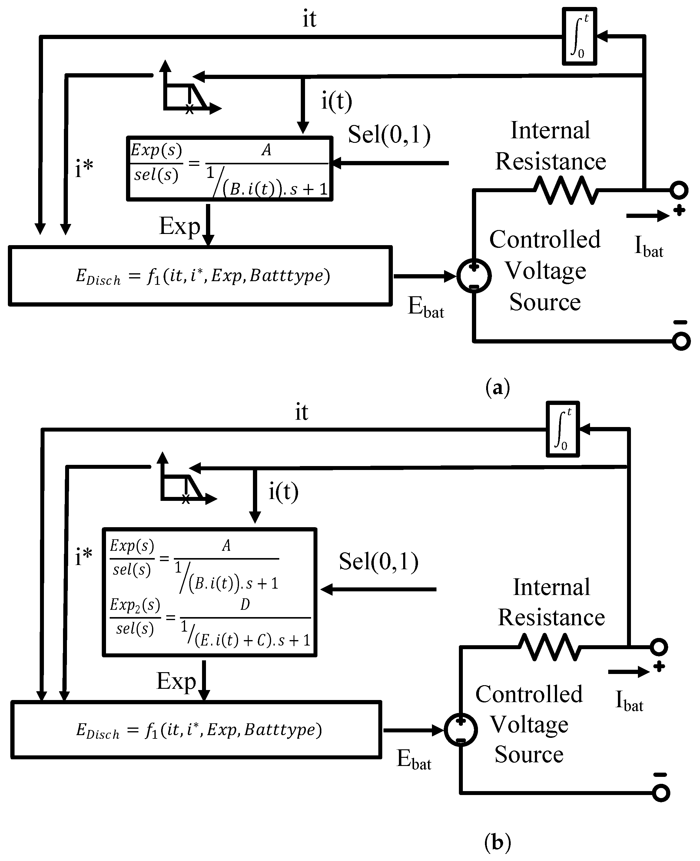
2. Generic Battery Model

2.1. Standard Generic Battery Model

Figure 1a shows the equivalent circuit for the generic battery dynamic model that can be used for the most rechargeable battery types. In this paper, lithium-ion battery type is chosen, and the model uses the following equation for lithium-ion battery type in the discharging mode:

$$f_1(it,i^{*},Exp,Li-ion)=E_0-K\frac{Q}{Q-it}{i}^{*}-K\frac{Q}{Q-it}it+A{e}^{(-Bit)},$$

(1)

where $it$ is extracted battery capacity, $i^{*}$ is the low-frequency current dynamics, i is battery current, $Exp(·)$ represents exponential zone dynamics, $E_0$ is the initial operating battery voltage which represents the full charge value. k is the polarization constant (represented as $k_1$) or polarization resistance (represented as $k_2$), Q is the maximum battery capacity, A is exponential zone amplitude, and b is Exponential zone time constant inverse.

2.2. Proposed Generic Battery Models

A general equivalent circuit for the proposed generic battery models is shown in Figure 1b. The models and their equation are described in

Table 1. Models Equation.

Model	Equations	Differences
1.	$V_{bat}=v_0-kim-kym+a{e}^z$	Reference model.
2.	$V_{bat}=v_0-ir$ $-k_{1}im-(k_1+k_2)m-k_{2}ym$ $+a{e}^z+d{e}^{ey+c}$	$km(i-y)$.
3.		$ir$ term.
4.		$q=q_0+{\alpha }_{1}t+{\alpha }_2{t}^2$. $r=r_0+{\beta }_{1}t+{\beta }_2{t}^2$.
5.		$(k_1+k_2)m$.
6.		$a{e}^{by}$
7.		$a{e}^{by+c}$
8.		$a{e}^{-by}+d{e}^{ey+c}$

, where $y={\int }_0^{t}tdt$, $m=\frac{q}{q-y}$ and $z=-by$.

Table 2. The Proposed Generic Models.

Model	Parameters										# Parameters
	Common	r	$K_2$	${\alpha }_1$	${\alpha }_2$	${\beta }_1$	${\beta }_2$	c	d	e
1	$V_o$ $K_1$ a b q										5
2		✓									6
3		✓	✓								7
4		✓	✓	✓	✓	✓	✓				11
5		✓	✓	✓	✓	✓	✓				11
6		✓	✓	✓	✓	✓	✓				11
7		✓	✓	✓	✓	✓	✓	✓			12
8		✓	✓	✓	✓	✓	✓	✓	✓	✓	14

indicates the difference between each model, the parameters used, and their number.

• Model 1 is the reference model, where it has 5 parameters only, which are $V_o$, k, a, b, and q;
• Model 2 has the same equation as the reference model, except it has the k constant as two independent constants since they represent the polarization constant in V/Ah and the polarization resistance in $\Omega$, as witnessed in [15];
• Model 3 has $ir$ as an additional term to the previous equation to consider the battery resistance;
• Model 4 has $q=q_0+{\alpha }_{1}t+{\alpha }_2{t}^2$, and $r=r_0+{\beta }_{1}t+{\beta }_2{t}^2$. It takes into account the aging effect on battery capacity and resistance;
• Model 5 adds $(k_1+k_2)m$ term to the previous equation. It tries to find the polarization constant and resistance effects with the current battery capacity.

Models 6, 7, and 8 try to find the effect of the exponential term on the final curve.

• Model 6 replaces the exponential term—in the previous equation—with a positive one;
• Model 7 adds the constant c to the positive exponential term;
• Model 8 has negative and positive exponential terms with the constant c.

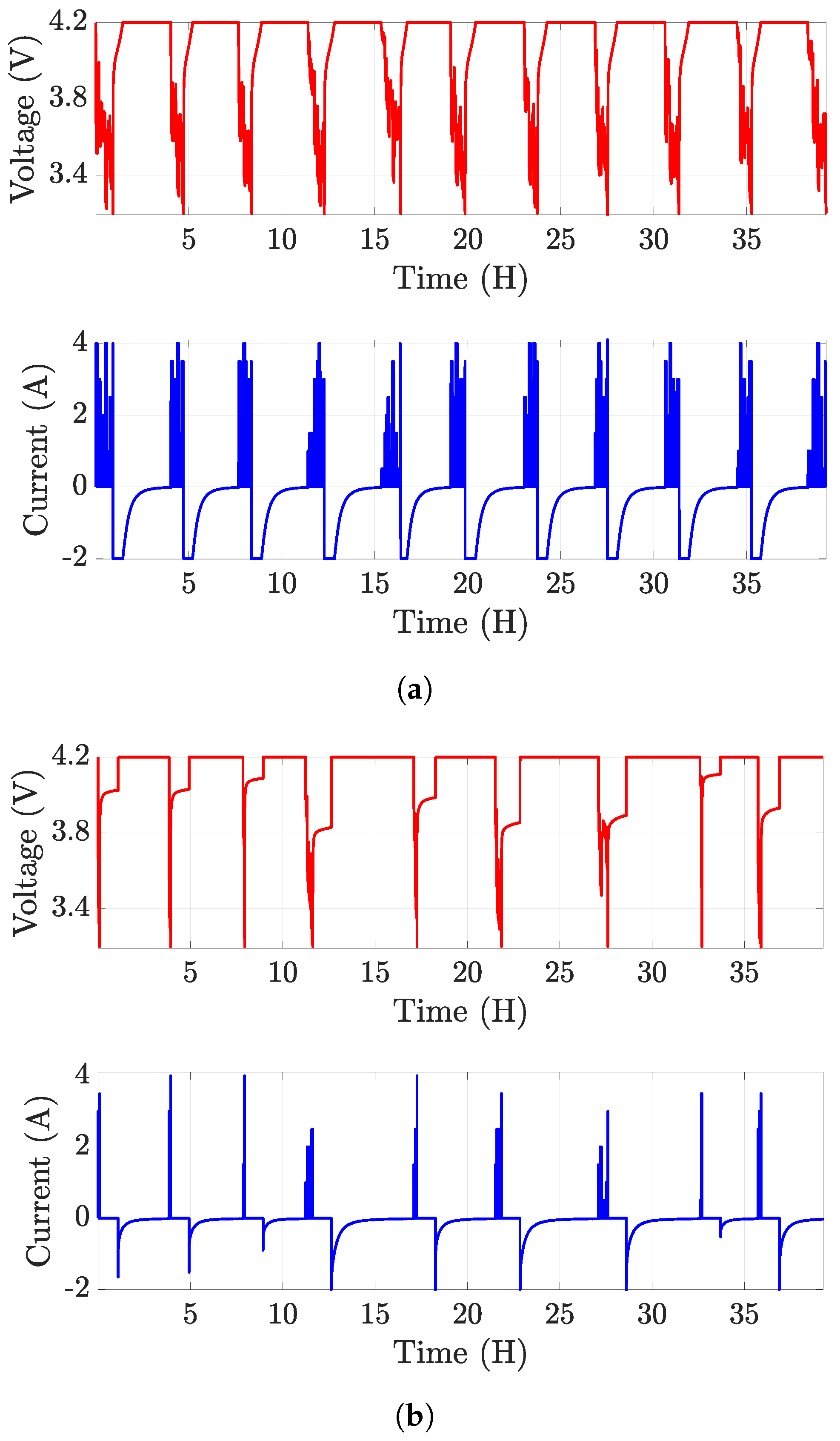
2.3. NASA Room Temperature Random Walk Discharging Datasets

A set of long-term (more than 50 h) published data was utilized to test the standard and the proposed models. Four lithium-ion batteries were repeatedly charged to 4.2 V and then discharged to 3.2 V using a randomized series of discharging currents between 0.5 A and 4 A. This discharging profile is annotated as “random walk (RW) discharging”. The RW discharge profiles are made up of intervals of battery resting (zero current) and 5-minute battery discharges at a specific current. Figure 2 presents the voltage and current test profiles.

2.4. Marine Predator Algorithm

The Marine Predators Algorithm, MPA, has been recently proposed by [27] as a biologically inspired optimization algorithm. It models interactions between marine prey and predators using governing strategies for optimal foraging and memory in predators. Further, marine predators have been discovered to use Levy and Brownian motions in habitats with low and high prey populations, respectively. However, when individuals move through numerous places throughout their lives, they apply both RW approaches. Utilizing their great memory, predators constantly remind themselves and those around them of crucial details [27].

Similar to the majority of meta-heuristic algorithms, the MPA population is started by taking samples from a uniform distribution throughout the viable area of the search space. The Prey and Elite matrices are then developed, which are two crucial matrices. The dimensions of both matrices are $ntimesd$, where n is the total number of search agents and d is the search space size. The prey positions from the starting stage are initially included in the rows of the Prey matrix. The Prey matrix updating strategy will then differ based on the optimization stage. Whenever the Elite matrix is constructed, the top predator’s location is duplicated across all rows [27,28].

2.5. Problem Formulation

In the parameter identification problem, the objective function is considered as the average normalized absolute error. The MPA optimizer aims to minimize this objective function, which is defined as:

$$\begin{array}{cc}\hfill f_{min}& =\frac{1}{N}\sum _{i=1}^N\left|\frac{V_{est}\left(t_i\right)-V_{meas}\left(t_i\right)}{V_{meas}\left(t_i\right)}\right|,\hfill \end{array}$$

(2)

where $V_{est}$ is the estimated voltage value at a specific time $t_i$, $V_{meas}$ is the measured voltage value, from each RW dataset, at the same time, and N is the number of time samples. In the problem, MPA is employed to find each model parameter. For Model 1, the search space vector is decided to be: [$V_o$ K a b q]. The search agent’s number is 10 times the search space dimension. Therefore, the number of search agents is 50 for Model 1. For Models 2, 3, 4, 5, 6, 7, and 8, the search space vector is [$V_o$ K a b q r], [$V_o$ $K_1$ $K_2$ a b q r], [$V_o$ $K_1$ $K_2$ a b q r ${\alpha }_1$ ${\alpha }_2$ ${\beta }_1$ ${\beta }_2$], [$V_o$ $K_1$ $K_2$ a b q r ${\alpha }_1$ ${\alpha }_2$ ${\beta }_1$ ${\beta }_2$], [$V_o$ $K_1$ $K_2$ a b q r ${\alpha }_1$ ${\alpha }_2$ ${\beta }_1$ ${\beta }_2$], [$V_o$ $K_1$ $K_2$ a b q r ${\alpha }_1$ ${\alpha }_2$ ${\beta }_1$ ${\beta }_2$ c], and [$V_o$ $K_1$ $K_2$ a b q r ${\alpha }_1$ ${\alpha }_2$ ${\beta }_1$ ${\beta }_2$ c d e], respectively. The search agents are 60, 70, 110, 110, 110, 120, and 140 for the proposed models in order.

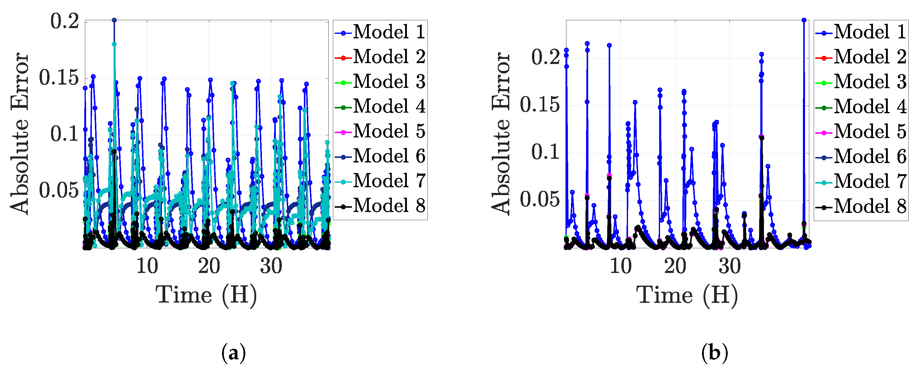
3. Results and Discussion

Table 3. First RW Model Results.

Model	Fitted Plot	${\mathit{V}}_{\mathit{o}}-\mathit{ir}$	${\mathit{k}}_1\mathit{im}$	$({\mathit{k}}_1+{\mathit{k}}_2)\mathit{m}$	${\mathit{k}}_2\mathit{ym}$
1
2
3
4
5
6
7
8

and

Table 4. Cont. First RW Model Results.

Model	${\mathit{ae}}^{\mathit{b}\mathit{y}}$	${\mathit{ae}}^{\mathit{b}\mathit{y}+\mathit{c}}$	${\mathit{ae}}^{-\mathit{b}\mathit{y}}$	${\mathit{de}}^{\mathit{e}\mathit{y}+\mathit{c}}$
1
2
3
4
5
6
7
8

, and

Table 5. Last RW Model Results.

Model	Fitted Plot	${\mathit{V}}_{\mathit{o}}-\mathit{ir}$	${\mathit{k}}_1\mathit{im}$	$({\mathit{k}}_1+{\mathit{k}}_2)\mathit{m}$	${\mathit{k}}_2\mathit{ym}$
1
2
3
4
5
6
7
8

and

Table 6. Cont. last RW Model Results.

Model	${\mathit{ae}}^{\mathit{b}\mathit{y}}$	${\mathit{ae}}^{\mathit{b}\mathit{y}+\mathit{c}}$	${\mathit{ae}}^{-\mathit{b}\mathit{y}}$	${\mathit{de}}^{\mathit{e}\mathit{y}+\mathit{c}}$
1
2
3
4
5
6
7
8

provide the fitted curves for the first and last RW datasets, respectively. They demonstrate the best fit for the proposed models to the chosen datasets. Moreover, as seen in Table 3, most models almost fit by an absolute error of $0.0057$. All of the suggested models outperform the standard model which cannot fit the upper half of the data, as shown in Table 3 and Table 5. The fitting behavior of the other models is almost comparable; the few differences are visible in the plot’s details. Moreover, this behavior is valid for all models except Models 6 and 7, which act differently in the upper portion, hitting $4.4$ V every cycle. For the first dataset, Models 4, 5, and 8 are the best-fitted models, as shown by the absolute error plot in Figure 3a, and they also have the lowest $f_{min}$. The fitted plots for the last RW dataset are displayed in the first column of Table 5, where the best fit is Model 7.

The standard model displays the most significant absolute error across each cycle for the first RW dataset, where it is practically constant at $0.15$. The rest of the models, in contrast, only exhibit absolute peak error at the 5 H cycle and have significantly lower values for the remaining cycles. Even so, the maximum absolute error for Models 2, 3, 4, 5, and 8 is $0.08$, whereas the absolute error for the remaining cycles is $0.03$. Model 6 has a $0.2$ peak absolute error. The remaining cycles of Models 3, 4, and 5 have a value of $0.3$, while the cycles of Models 6 and 8 have values of $0.1$ and $0.01$, respectively. The absolute error values of Model 7 are variable, with a maximum of $0.3$ and other cycles ranging from $0.14$ to $0.06$.

For the last RW dataset, the standard model also has the largest absolute error of $0.2$ for most of the cycles. All models have nearly the same absolute curve, where they peak at $0.102$ and $0.02$ for most cycles. The models’ peak absolute error is at 35 H cycle. The curves also have two spikes at 5 H and 9 H cycles with absolute errors of $0.06$ and $0.08$, respectively.

According to

Table 7. First RW cycles Parameters’ values for the proposed models.

	Model Number	1	2	3	4	5	6	7	8
Parameter
$V_0$ (V)		$3.4$	$3.57$	$3.57$	$3.57$	$3.57$	$4.03$	$3.03$	$0.46$
$K_1$ (V/Ah)		4.49$\times {10}^{-5}$	$15.83$	2.38$\times {10}^{-7}$	$1.88$	0	$14.95$	4.73$\times {10}^{-6}$	$6.86$
$K_2$ ($\Omega$)				2.38$\times {10}^{-6}$	$0.36$	1.02$\times {10}^{-8}$	$0.0017$	$1.21$	4.03$\times {10}^{-6}$
a (Ah)${}^{-1}$		$0.78$	$0.62$	$0.62$	$0.623$	$0.62$	0	$0.92$	$0.62$
b (V)		5.76$\times {10}^{-4}$	2.43$\times {10}^{-4}$	$2.43$	2.4$\times {10}^{-4}$	2.4$\times {10}^{-4}$	$0.0125$	0	2.4$\times {10}^{-4}$
q (Ah)		$1.56$	1.07$\times {10}^{-4}$	$4.87$	$0.00129$	$0.28$	1.1$\times {10}^{-4}$	$0.00159$	1.42$\times {10}^{-5}$
r ($\Omega$)			$0.13$		$0.13$	$0.13$	$0.18$	$0.17$	$0.13$
${\alpha }_1$					0	1	0	7.3$\times {10}^{-7}$	0
${\alpha }_2$					0	$0.001$	0	0	0
${\beta }_1$					2.55$\times {10}^{-8}$	2.05$\times {10}^{-8}$	0	0	2.56$\times {10}^{-8}$
${\beta }_2$					0	0	0	0	0
c								$0.02$	$0.03$
d									$3.01$
e									0
$fmin$		$0.0406$	$0.005.8$	$0.0058$	$0.0057$	$0.0057$	$0.0377$	$0.0374$	$0.0057$

, $v_o$ values range from 3 to 4 V, except in the case of Model 8, where $v_o$ equals $0.5$ V. $K_1$ ranges from pV/Ah, where Model 4 equals $0.35$ pV/Ah, and terminate at 16 V/Ah in Model 8. Additionally, the value for Model 2 is $0.23$ $\mathsf{\mu }$V/Ah, for Model 6, it is $4.7$ $\mathsf{\mu }$V/Ah, and for Model 1, it is $4.05$ $\mathsf{\mu }$V/Ah. Consequently, for Models 3 and 7, $K_1$ eauals $1.88$ and $6.8$, respectively, in terms of V/Ah. Despite that, there are no reliable data for the polarisation resistance, $K_2$. For Model 4, it is equal to $0.1$ n$\Omega$, and for Models 6 and 2, it is equal to $1.2$ and $2.3$ $\mathsf{\mu }\Omega$. Following that, $K_2$ equals $1.7$ mV for Model 5. Last but not least, $0.3$ and $1.2$ V correspondingly for Models 3 and 7. a, in (Ah)${}^{-1}$, is nearly constant at $0.62$. It is nearly zero at Model 5. Models 1 and 6 have values of $0.78$ and $0.92$, respectively. For the majority of models, b has constant values at $0.24$ mV. The value of Model 7 is very close to zero. Models 1 and 6 have values of $0.57$ and 120 in mV, respectively. The Model 3 value, however, is the highest at $2.43$ V. For q, in Ah, Models 2, 6, 4, and 7 have values $0.1$, $0.11$, $1.29$, and $1.58$. Additionally, the values for Models 5, 1, and 3 are $0.28$, $1.56$, and $4.87$, respectively. The battery resistance in $\Omega$, r, almost always equals $0.13$, except for Models 7 and 6, for which it is, respectively, $0.17$ and $0.18$. Except for Model 5, ${\alpha }_1$ and ${\alpha }_2$, t coefficients for q, have very small values.

In Table 3, $V_o-ir$ term has the same pattern among all models for the first RW dataset. However, it differs in its peaks and troughs. Excluding Models 7 and 8, all models peaked around $3.8$ V and troughed around 3 V. Models 7 and 8 reached their highest point at $3.5$ V and their lowest point at $2.1$ and $2.1$ and $-0.06$ V, respectively. Each model’s $k_{1}im$ term has a unique form and set of values. Model 5, for example, has a reciprocal shape for the $V_o-ir$ term in the same model. Other models have different spike values with time. The lowest valued models are 5 and 7, which are in the nano range. Whereas, Models 4, 1, and 8 have the highest values. Model 7 has the highest value in the $(k_1+k_2)m$ term, with a peak value of 30 mV. Multiple peaks are present in various periods with random forms, some of which are in the negative part. Low values in the micro range are found for Models 5 and 8, whose peaks are 20 $\mathsf{\mu }$V and 50 $\mathsf{\mu }$V, respectively. Models 5 and 6 peak at the beginning of the period, but the curve thereafter follows a straight line until the end of the period. $K_{2}ym$ term takes the form of straight lines with minor swings, a pulse followed by a straight line, or a straight line with a slope. Additionally, the values range from picovolts to millivolts. For instance, Model 7 has a straight line with a negative slope and a peak of $-20$ mV. Models 2 and 4 have the same shape, but Model 2’s voltage value is $-1.6$ mV, while Model 4’s voltage value is $-470$ mV. The pulse of Model 8, which has a value of $-0.57$ pV, is present at the start of the timeline and varies somewhat along it. Model 6 is the next model, with a value of $0.18$ $\mathsf{\mu }$V. Finally, the values of Models 5 and 3 are 1 and 100 mV, respectively.

In Table 4, the $a{e}^{by}$ term in Model 6 has relatively low values. Along the time frame, it has several pulses with varied values. In Model 7, term $a{e}^{by+c}$ behaves as a straight line with voltage value 1 V. Except for Model 5, all models have the same form for the $a{e}^{-by}$ term, which has many peaks throughout time. They also share the same voltage values, ranging from $0.2$ to $0.6$ V. Model 1 has a $0.2$ V higher than the rest. Model 5, nevertheless, has extremely low voltage, ranging from 0 to 6 $\mathsf{\mu }$V. In Model 8, the term $d{e}^{ey+c}$ behaves as a straight line at $3.1$ V.

In Table 5, the last RW dataset shows that $V_o$ fluctuates somewhat. Models 6, 1, and 7 have voltages of $1.57$, $2.63$, and $3.38$ volts, respectively. However, Models 2, 3, 4, and 5 have equal values. The value of Model 8 is the lowest, coming in at $0.57$ mV. Similar to those in the Frist dataset, $K_1$ has low values as in the range of $\times {10}^{-14}$ for Models 2 and 6. Models 8, 4, and 7 are next, with, correspondingly, $0.28$, $0.34$, and $0.56$ nV/Ah. 37 nV/Ah is the Model 1 value. The values for Models 3 and 5 are, respectively, $0.54$ and $0.12$ mV/Ah. $K_2$ values range from nearly zero to millivolts. Models 4 and 5 have the lowest values. Model 3, which is in the microvolt range, comes next and then Models 6, 7, and 8, which are in the millivoltage range. The values for Models 2, 3, 4, and 5 are equal, indicating some stability in a values. The value of Model 7 is $0.15$ (Ah)${}^{-1}$, while the value of Model 8 is $4.17$ (Ah)${}^{-1}$. The constant b has the highest and lowest values in Models 4 and 8, respectively, compared to the other dataset. Other models are measured in mV. q values have some consistency, where most models are in mAh. Nonetheless, Models 1 and 3 are valued more than others, at $1.38$ and $4.32$, respectively. At $0.25$$\Omega$, the values of r remain constant. Except for Model 5, all models have an ${\alpha }_1$ of 1. The same holds for ${\alpha }_2$. While ${\beta }_2$ roughly equates to zero, ${\beta }_1$ values are low compared to the other values, falling to ${10}^{-8}$. The values for $f_{m}in$ are similar. For example, the values of Models 4, 5, and 6 are all $0.0071$, while those of Models 2 and 3 are $0.0072$. Model 6 has the highest value among the suggested models, equaling $0.037$.

On the other hand, for the last RW dataset in Table 5, all models except Models 7 and 8 have the same form, peaks, and troughs for the $V_o-ir$ term. The peak values for the models are $1.5$ V and $0.8$ V, while the trough values are $0.6$ V and $-0.005$ V, respectively. They have the same shape as those in the first dataset but have different peak values. Peaks and troughs for the remaining models are $3.8$ V and $2.6$ V. Except for Models 7 and 8, which are identical, no model with $k_{1}im$ term has a constant shape. Further, Models 7 and 8 have the highest values, 7 mV and 5 mV, as peaks for the models, respectively. Model 4 has the lowest value and goes up to 1 nV. The behavior of Models 3 and 6 is the same with the same values, with peaks and troughs of 100 $\mathsf{\mu }$V and $-100$ $\mathsf{\mu }$V, respectively. Model 7 has relatively low values in the micro range.

Roughly all models have the same shape for the $(k_1+k_2)m$ term, which has a pulse in the first time slot and then continues in a straight line with slight fluctuations. Except for Model 5, whose peak equals $1.2$ V, its values range in mV. Peak values for Models 7, 6, and 8 are, respectively, $0.3$, $0.5$, and $1.9$ mV as shown in

Table 8. Last RW cycles Parameters’ values for the proposed models.

	Model	1	2	3	4	5	6	7	8
Parameter
$V_0$ (V)		$2.63$	$3.57$	$3.57$	$3.57$	$3.57$	$1.57$	$3.38$	5.73$\times {10}^{-4}$
$K_1$ (V/Ah)		3.79$\times {10}^{-5}$	0	5.46$\times {10}^{-4}$	3.44$\times {10}^{-8}$	1.22$\times {10}^{-4}$	0	5.6$\times {10}^{-8}$	2.84$\times {10}^{-8}$
$K_2$ ($\Omega$)				1.62$\times {10}^{-6}$	0	0	5.95$\times {10}^{-4}$	4.16$\times {10}^{-4}$	2.28$\times {10}^{-4}$
a (Ah)${}^{-1}$		$1.58$	$0.64$	$0.64$	$0.63$	$0.63$	$2.63$	$0.15$	$4.17$
b (V)		2.21$\times {10}^{-4}$	3.69$\times {10}^{-4}$	3.68$\times {10}^{-4}$	$3.69$	3.69$\times {10}^{-4}$	1.41$\times {10}^{-4}$	2.38$\times {10}^{-4}$	2.35$\times {10}^{-7}$
q (Ah)		$1.38$	$0.58$	$4.32$	$0.71$	$0.12$	$0.08$	$0.04$	$0.09$
r ($\Omega$)			$0.25$		$0.25$	$0.25$	$0.25$	$0.25$	$0.25$
${\alpha }_1$					$0.99$	$0.3$	1	1	1
${\alpha }_2$					$0.93$	$0.008$	1	1	1
${\beta }_1$					3.91$\times {10}^{-8}$	9.91$\times {10}^{-9}$	4.76$\times {10}^{-8}$	4.49$\times {10}^{-8}$	4.3$\times {10}^{-8}$
${\beta }_2$					0	0	0	0	0
c								$1.68$	$10.85$
d									5.4$\times {10}^{-7}$
e									8.44$\times {10}^{-4}$
$f_{min}$		$0.0474$	$0.0072$	$0.0072$	$0.0071$	$0.0071$	$0.0377$	$0.0061$	$0.0071$

. $K_{2}ym$ term typically has numerous peaks along the timeline, each with a different value. For instance, the shapes of Models 4, 6, and 7 are identical, as well as those of 1, 2, and 3. Model 5, on the other hand, behaves like a low-pass filter, producing a voltage pulse at the beginning of the timeline and a gradual attenuation toward the end. Voltage for this term is very low. Model 4’s value is equal to 0 mV, and Model 2’s value is 0 mV. Models 8, 5, 6, and 7 are thus equal to $0.3$ V, $1.2$ V, $1.5$ V, and 2 V, respectively.

In Table 6, $a{e}^{by}$ term behaves similarly to $K_{2}ym$ in the same model. Nevertheless, its values are higher than those in the first dataset. Its maximum value is $3.8$ V. It also features several peaks that cycle throughout time, ranging from $2.8$ V to $3.6$ V. $a{e}^{by+c}$ term has multiple peaks during the timeline. Its maximum value is $4.5$ V, and its minimum value is 4 V. There are 3 alternative plot forms for $a{e}^{-by}$ term. Models 1 to 4 all have the same shape, whereas 5 and 8 have different shapes. Models 3 and 4 are common in their shape and voltage ranging from $0.3$ V to $0.6$ V. The lowest value in the picovolts region belongs to Model 5. On the other hand, the highest one, which equals $1.6$ as a peak, is found in Model 1. The voltage ranges for Models 2 and 8 are $0.4$ V to $0.6$ V and $0.05$ V to $0.15$ V, respectively. $d{e}^{ey+c}$ term acts similarly to the $K_{2}ym$ term in the same model but at different voltage values ranging at $3.5$ V.

4. Conclusions

Seven dynamic generic models for characterizing well lithium-ion batteries are proposed. In addition, a detailed look at each term in each model’s equations to better understand its effect on the fitted curve is introduced. Using the MPA algorithm and NASA RW discharging dataset, the fitted results of the proposed models were obtained and compared to those of the Standard model. For the first RW data set, the best-fitting models are 4, 5, and 8, which account for the impact of aging on battery capacity and resistance. Also noted are the polarization constant and resistance effects in Model 5, as well as the negative and positive exponential components in Model 8. Model 7 is the top performing model on the last RW dataset, with $0.0061$$f_{min}$. It considers the influence of polarization, the aging of the battery, and the positive exponential-term effects.

The performance properties of lithium-ion batteries are temperature-sensitive [29]. The recoverable power and capacity may be decreased dramatically when used or stored at temperatures over 50 °C [30]. On the other hand, when the battery is charged at temperatures below $-10$ °C, lithium plating reduces capacity. These low temperatures diminish extractable energy [29]. Hence, lithium-ion batteries used in electric vehicle and hybrid electric vehicles applications must be kept below 50 °C but promptly heated or self-heated by cycling within permitted limits before functioning at cold temperatures [31]. For future work, other datasets and testing scenarios will be considered, in addition to studying different battery issues, including thermal issues.

References

1. Thakur, A.K.; Prabakaran, R.; Elkadeem, M.; Sharshir, S.W.; Arıcı, M.; Wang, C.; Zhao, W.; Hwang, J.Y.; Saidur, R. A state of art review and future viewpoint on advance cooling techniques for Lithium–ion battery system of electric vehicles. J. Energy Storage 2020, 32, 101771. [Google Scholar] [CrossRef]
2. Armand, M.; Tarascon, J. Issues and challenges facing rechargeable lithium batteries. Nature 2001, 414, 359–367. [Google Scholar]
3. Liu, Z.; He, H.; Xie, J.; Wang, K.; Huang, W. Self-discharge prediction method for lithium-ion batteries based on improved support vector machine. J. Energy Storage 2022, 55, 105571. [Google Scholar] [CrossRef]
4. Wang, Y.; Liu, B.; Li, Q.; Cartmell, S.; Ferrara, S.; Deng, Z.D.; Xiao, J. Lithium and lithium ion batteries for applications in microelectronic devices: A review. J. Power Sources 2015, 286, 330–345. [Google Scholar] [CrossRef] [Green Version]
5. Allagui, A.; Freeborn, T.J.; Elwakil, A.S.; Fouda, M.E.; Maundy, B.J.; Radwan, A.G.; Said, Z.; Abdelkareem, M.A. Review of fractional-order electrical characterization of supercapacitors. J. Power Sources 2018, 400, 457–467. [Google Scholar] [CrossRef]
6. AbdelAty, A.; Fouda, M.E.; Elbarawy, M.T.; Radwan, A. Optimal charging and discharging of supercapacitors. J. Electrochem. Soc. 2020, 167, 110521. [Google Scholar] [CrossRef]
7. AbdelAty, A.; Fouda, M.; Elbarawy, M.; Attia, H.; Radwan, A. Parameter Identification of Flexible Supercapacitors with Fractional Cuckoo Search. In Proceedings of the IEEE 2020 32nd International Conference on Microelectronics (ICM), Aqaba, Jordan, 14–17 December 2020; pp. 1–4. [Google Scholar]
8. Fouda, M.E.; Elwakil, A.S.; Allagui, A.; Rezk, H.; Nassef, A.M. Communication—Convolution-Based Estimation of Supercapacitor Parameters under Periodic Voltage Excitations. J. Electrochem. Soc. 2019, 166, A2267. [Google Scholar] [CrossRef]
9. Fouda, M.; Elwakil, A.; Radwan, A.; Allagui, A. Power and energy analysis of fractional-order electrical energy storage devices. Energy 2016, 111, 785–792. [Google Scholar] [CrossRef]
10. Jiang, Y.; Xia, B.; Zhao, X.; Nguyen, T.; Mi, C.; de Callafon, R.A. Data-based fractional differential models for non-linear dynamic modeling of a lithium-ion battery. Energy 2017, 135, 171–181. [Google Scholar] [CrossRef]
11. Waag, W.; Käbitz, S.; Sauer, D.U. Application-specific parameterization of reduced order equivalent circuit battery models for improved accuracy at dynamic load. Measurement 2013, 46, 4085–4093. [Google Scholar] [CrossRef]
12. Tremblay, O.; Dessaint, L.A. Experimental validation of a battery dynamic model for EV applications. World Electr. Veh. J. 2009, 3, 289–298. [Google Scholar] [CrossRef] [Green Version]
13. Sasaki, T.; Ukyo, Y.; Novák, P. Memory effect in a lithium-ion battery. Nat. Mater. 2013, 12, 569–575. [Google Scholar] [CrossRef] [PubMed]
14. Romanenko, K.; Jerschow, A. Observation of memory effects associated with degradation of rechargeable lithium-ion cells using ultrafast surface-scan magnetic resonance imaging. J. Mater. Chem. A 2021, 9, 21078–21084. [Google Scholar] [CrossRef]
15. Prieto, R.; Oliver, J.; Reglero, I.; Cobos, J. Generic battery model based on a parametric implementation. In Proceedings of the IEEE 2009 Twenty-Fourth Annual IEEE Applied Power Electronics Conference and Exposition, Washington, DC, USA, 15–19 February 2009; pp. 603–607. [Google Scholar]
16. Hannan, M.; Azidin, F.; Mohamed, A. Hybrid electric vehicles and their challenges: A review. Renew. Sustain. Energy Rev. 2014, 29, 135–150. [Google Scholar] [CrossRef]
17. Song, D.; Sun, C.; Wang, Q.; Jang, D. A generic battery model and its parameter identification. Energy Power Eng. 2018, 10, 10. [Google Scholar] [CrossRef] [Green Version]
18. Tremblay, O.; Dessaint, L.A.; Dekkiche, A.I. A Generic Battery Model for the Dynamic Simulation of Hybrid Electric Vehicles. In Proceedings of the 2007 IEEE Vehicle Power and Propulsion Conference, Arlington, TX, USA, 9–12 September 2007; pp. 284–289. [Google Scholar] [CrossRef]
19. Scipioni, R.; Jørgensen, P.S.; Graves, C.; Hjelm, J.; Jensen, S.H. A physically-based equivalent circuit model for the impedance of a LiFePO4/graphite 26650 cylindrical cell. J. Electrochem. Soc. 2017, 164, A2017. [Google Scholar] [CrossRef] [Green Version]
20. De Lima, A.B.; Salles, M.B.; Cardoso, J.R. State-of-charge estimation of a li-ion battery using deep forward neural networks. arXiv 2020, arXiv:2009.09543. [Google Scholar]
21. Bhattacharjee, A.; Verma, A.; Mishra, S.; Saha, T.K. Estimating state of charge for xEV batteries using 1D convolutional neural networks and transfer learning. IEEE Trans. Veh. Technol. 2021, 70, 3123–3135. [Google Scholar] [CrossRef]
22. Kollmeyer, P. Panasonic 18650pf li-ion battery data. Mendeley Data 2018, 1. [Google Scholar]
23. Kollmeyer, P.; Vidal, C.; Naguib, M.; Skells, M. Lg 18650HG2 li-ion battery data and example deep neural network xEV SOC estimator script. Mendeley Data 2020, 3, 2020. [Google Scholar]
24. Ely, J.J.; Koppen, S.V.; Nguyen, T.X.; Dudley, K.L.; Szatkowski, G.N.; Quach, C.C.; Vazquez, S.L.; Mielnik, J.J.; Hogge, E.F.; Hill, B.L.; et al. Radiated Emissions From a Remote-Controlled Airplane-Measured in a Reverberation Chamber; Technical report; 2011. Available online: https://ntrs.nasa.gov/api/citations/20110011513/downloads/20110011513.pdf (accessed on 1 March 2023).
25. Hogge, E.F.; Bole, B.M.; Vazquez, S.L.; Celaya, J.R.; Strom, T.H.; Hill, B.L.; Smalling, K.M.; Quach, C.C. Verification of a remaining flying time prediction system for small electric aircraft. In Proceedings of the Annual Conference of the PHM Society, Coronado, CA, USA, 18–24 October 2015; Volume 7. [Google Scholar]
26. Bole, B.; Kulkarni, C.; Daigle, M. Randomized battery usage data set. NASA AMES Progn. Data Repos. 2014, 70. [Google Scholar]
27. Faramarzi, A.; Heidarinejad, M.; Mirjalili, S.; Gandomi, A.H. Marine Predators Algorithm: A nature-inspired metaheuristic. Expert Syst. Appl. 2020, 152, 113377. [Google Scholar] [CrossRef]
28. Yousri, D.; Babu, T.S.; Beshr, E.; Eteiba, M.B.; Allam, D. A Robust Strategy Based on Marine Predators Algorithm for Large Scale Photovoltaic Array Reconfiguration to Mitigate the Partial Shading Effect on the Performance of PV System. IEEE Access 2020, 8, 112407–112426. [Google Scholar] [CrossRef]
29. Bandhauer, T.M.; Garimella, S.; Fuller, T.F. A critical review of thermal issues in lithium-ion batteries. J. Electrochem. Soc. 2011, 158, R1. [Google Scholar] [CrossRef]
30. Liu, H.; Wei, Z.; He, W.; Zhao, J. Thermal issues about Li-ion batteries and recent progress in battery thermal management systems: A review. Energy Convers. Manag. 2017, 150, 304–330. [Google Scholar] [CrossRef]
31. Bibin, C.; Vijayaram, M.; Suriya, V.; Ganesh, R.S.; Soundarraj, S. A review on thermal issues in Li-ion battery and recent advancements in battery thermal management system. Mater. Today Proc. 2020, 33, 116–128. [Google Scholar] [CrossRef]
Figure 1. (a) Generic battery model equivalent circuit and (b) the proposed generic battery model equivalent circuit.
Electronics 12 01478 g001
Figure 2. Voltage and Current test profiles for the (a) first RW cycles and (b) last RW cycles.
Electronics 12 01478 g002
Figure 3. The absolute error for the proposed models (a) first RW data, and (b) last RW data.
Electronics 12 01478 g003